11institutetext: Aalto University
Department of Mathematics and Systems Analysis
11email: firstname.lastname@aalto.fi

Reduced Complexity Decoding of $n\times n$ Algebraic Spaceโ€“Time Codes

Amaro Barreal โ€ƒโ€ƒ Camilla Hollanti โ€ƒโ€ƒ David Karpuk The authors are financially supported by Academy of Finland grants #276031, #282938, #283262 and #268364, and a grant from Magnus Ehrnrooth Foundation, Finland. The support from the European Science Foundation under the COST Action IC1104 is also gratefully acknowledged.
Abstract

Algebraic spaceโ€“time coding allows for reliable data exchange across fading multiple-input multiple-output channels. A powerful technique for decoding spaceโ€“time codes is Maximum-Likelihood (ML) decoding, but well-performing and widely-used codes such as the Golden code often suffer from high ML-decoding complexity. In this article, a recursive algorithm for decoding general algebraic spaceโ€“time codes of arbitrary dimension is proposed, which reduces the worst-case decoding complexity from $O(|\mathcal{S}|^{n^{2}})$ to $O(|\mathcal{S}|^{n})$.

1 Introduction

Algebraic Spaceโ€“Time (ST) coding is a powerful technique for reliable data exchange across fading Multiple-Input Multiple-Output (MIMO) channels, which makes use of available multiple antennas at the transmitter and receiver, as well as multiple channel uses to introduce redundancy in the transmitted information. Data transmission across a MIMO channel can be modeled as

$$Y_{n_{r}\times T}=H_{n_{r}\times n_{t}}X_{n_{t}\times T}+N_{n_{r}\times T},$$ (1)

where the subscripts $n_{t}$, $n_{r}$ and $T$ denote the number of antennas at the transmitter, receiver, and the coding delay, respectively, $Y$ and $X$ are the received and sent matrices, $H$ is a random complex matrix modeling Rayleigh fading, and $N$ is a noise matrix whose entries are complex Gaussian with zero mean. In this paper we restrict ourselves to the fully symmetric case where $n_{t}=n_{r}=T=n$ for some $n$, and thus omit the above subscripts.

First introduced two decades ago, ST codes have been the subject of extensive study, and various algebraic criteria have been derived for ensuring reliable performance. The complexity of the decoding algorithm is a major issue in practical implementation. In digital video broadcasting [1], high decoding complexity prevents the use of high-rate space-time codes, since the complexity of linear decoders such as the sphere decoder grows exponentially in rank.

For the remainder of this article, we let $\operatorname{vec}:\operatorname{Mat}(m\times n,\mathbb{C})\to\mathbb{C}^{mn}$ be the vectorization transformation and we denote by $\mathcal{S}$ the signaling alphabet (e.g. $4$-QAM) used. Write vecโก(Hโ€‹X)=Gโ€‹svec๐ป๐‘‹๐บ๐‘ \operatorname{vec}(HX)=Gs, where sโˆˆ๐’ฎk๐‘ superscript๐’ฎ๐‘˜s\in\mathcal{S}^{k}. Decoding amounts to solving

argโ€‹minXโˆˆ๐’ณโ€‹โ€–Yโˆ’Hโ€‹Xโ€–F2โ†argโ€‹minsโˆˆ๐’ฎkโ€‹โ€–vecโก(Y)โˆ’Gโ€‹sโ€–2,leads-tosubscriptargmin๐‘‹๐’ณsuperscriptsubscriptnorm๐‘Œ๐ป๐‘‹๐น2subscriptargmin๐‘ superscript๐’ฎ๐‘˜superscriptnormvec๐‘Œ๐บ๐‘ 2\operatorname*{arg\,min}\limits_{X\in\mathcal{X}}{\left|\left|Y-HX\right|\right|_{F}^{2}}\leadsto\operatorname*{arg\,min}\limits_{s\in\mathcal{S}^{k}}{\left|\left|\operatorname{vec}(Y)-Gs\right|\right|^{2}}, (2)

where $||\cdot||_{F}$ and $||\cdot||$ denote the Frobenius and Euclidean norm, respectively. The latter search can be performed with the help of a sphere-decoder [2], whose decoding complexity is upper-bounded by $|\mathcal{S}|^{k}$.

Cleverly constructed algebraic ST codes known as fast-decodable codes reduce the complexity of ML-decoding by parallelizing the ML search (see e.g. [3]). However, ST codes exist that, although they do not allow for a reduced ML-decoding complexity, exhibit other desirable properties. An example of such a code is the Golden code [4], incorporated in the IEEE 802.16 (WiMAX) standard. The main algorithm of [5] reduces the decoding complexity of the Golden code from $O(|\mathcal{S}|^{3})$, corresponding to the complexity of ML-decoding, to $O(|\mathcal{S}|^{2})$, while maintaining nearly-ML performance. The algorithm is specific to the Golden code, but has been generalized to the $3\times 3$ and $4\times 4$ perfect codes in, respectively, [6] and [7]. The main contribution of this article is a recursive algorithm for decoding arbitrary $n\times n$ algebraic ST codes generalizing those of [5, 6, 7], which reduces the worst-case decoding complexity of $O(|\mathcal{S}|^{n^{2}})$ down to $O(|\mathcal{S}|^{n})$.

We review how algebraic ST codes are constructed from central simple algebras in Sectionย 2. Our algorithm for decoding general $n\times n$ algebraic ST codes is illustrated in Sectionย 3, wherein we also discuss its complexity. We then briefly consider the case $n=2$ and the Golden code as a special example in Sectionย 4. In Sectionย 5, we study the $4\times 4$ perfect code in more detail and provide an elementary statistical analysis of the involved quantities. While preliminary simulations seem to indicate that our algorithm has performance which is close to ML-decoding, time and space constraints prevent us from providing proper error rate simulations in this current draft. Detailed error rate simulation results will appear in a subsequent version of the paper.

2 Spaceโ€“Time Codes from Central Simple Algebras

Let $L/K$ be a Galois number field extension of degree $n$, and let $\mathcal{A}$ be a $K$-central simple $L$-algebra of rank $n$ over $L$, which we treat as a right $L$-vector space. For the rest of the article, we fix compatible embeddings of $K$ and $L$ into $\mathbb{C}$, and identify $K$ and $L$ with their images under these embeddings. To construct matrices to serve as codewords, we consider an injective algebra homomorphism

$$\rho:\mathcal{A}\to\operatorname{Mat}(n,\mathbb{C}).$$ (3)
Definition 1

An algebraic spaceโ€“time code is a finite subset $\mathcal{X}$ of $\rho(\mathcal{A})$ or its transpose $\rho(\mathcal{A})^{t}$.

As a general reference for applications of central simple algebras to space-time coding, we recommend [8], and as a catch-all mathematical reference for central simple algebras, we will use [9, Chapter IV]. There are many properties that can be desirable for an algebraic ST code, such as full-rank codewords, non-vanishing determinants, fast-decodability, balanced energy across transmitters, and optimal diversity-multiplexing tradeoff, which can be achieved by demanding some additional algebraic requirements of the involved structures.

Let us fix a basis $\{e_{1},\ldots,e_{n}\}$ of $\mathcal{A}$ as a right $L$-vector space. As an example of the above, consider the left regular representation (LRR), defined as follows. For fixed $x\in\mathcal{A}$, the map given by left multiplication $y\mapsto xy$ for all $y\in\mathcal{A}$ is right $L$-linear and compatible with algebra multiplication, and thus allows us to represent $x$ as a complex matrix $\rho(x)$ in the above basis. For notational convenience, we will below mostly consider the transpose of this representation.

To give a concrete example, consider the case where $L/K$ is a cyclic extension, whose Galois group $\text{Gal}(L/K)=\langle\sigma\rangle$ is generated by a single element. Fix some $\gamma\in K^{\times}$ and consider the central simple algebra

$$\mathcal{A}=\bigoplus_{j=0}^{n-1}e_{j}L$$ (4)

where the multiplication is determined by

$\displaystyle\lambda e_{j}$ $\displaystyle=e_{j}\sigma^{j}(\lambda)\quad\text{for all $\lambda\in L$, and}$ (5)
$\displaystyle e_{j}e_{k}$ $\displaystyle=\left\{\begin{array}[]{rll}e_{j+k}&\text{if}&j+k\leq n-1\\ e_{j+k-n}\gamma&\text{if}&j+k>n-1\end{array}\right.$ (8)

If $\rho$ denotes the LRR, the explicit structure of the codewords of $\mathcal{X}\subset\rho(\mathcal{A})^{t}$ can be found in, for example, [8]. More generally one can consider the left regular representation of the crossed-product algebra $\mathcal{A}(\varphi)$ for any $2$-cocycle $\varphi:\operatorname{Gal}(L/K)^{2}\rightarrow L^{\times}$ [9, Chapter IV].

Let us return to the general case of $L/K$ a Galois extension of degree $n$, and $\mathcal{A}$ any $K$-central simple $L$-algebra of rank $n$ over $L$. Consider any injective algebra homomorphism $\rho:\mathcal{A}\rightarrow\text{Mat}(n,\mathbb{C})$. The following decomposition of the matrix $\rho(x)^{t}$ for $x\in\mathcal{A}$ and its vectorization are central to our decoding algorithm.

Given $x\in\mathcal{A}$, we can represent it as $x=\sum_{j=1}^{n}e_{j}x_{j}$ for $x_{j}\in L$. If we fix $\{\omega_{1},\ldots,\omega_{n}\}$ to be a basis for $L$ as a $K$-vector space, then we can write $x$ as

$$x=\sum_{j=1}^{n}e_{j}x_{j}=\sum_{j=1}^{n}e_{j}\left(\sum_{i=1}^{n}\omega_{i}x_{ji}\right)=\sum_{i=1}^{n}\sum_{j=1}^{n}e_{j}\omega_{i}x_{ji},\quad\text{where $x_{ji}\in K$}$$ (9)

Passing to the transpose of the representation $\rho$ gives

$$\rho(x)^{t}=\sum_{i=1}^{n}\sum_{j=1}^{n}\rho(e_{j}\omega_{i}x_{ji})^{t}=\sum_{i=1}^{n}\rho(\omega_{i})^{t}\left(\sum_{j=1}^{n}\rho(e_{j})^{t}\rho(x_{ji})\right)$$ (10)

where we have used the fact that $\rho(x_{ji})$ is a scalar matrix and thus commutes with everything. If we define $X_{i}=\sum_{j=1}^{n}\rho(e_{j})^{t}\rho(x_{ji})$, then vectorizing $\rho(x)^{t}$ gives, by basic properties of the vectorization operator,

vecโก(ฯโ€‹(x)t)=โˆ‘i=1n(InโŠ—ฯโ€‹(ฯ‰i)t)โ€‹vecโก(Xi)=โˆ‘i=1n(InโŠ—ฯโ€‹(ฯ‰i)t)โ€‹ฮ“iโ€‹sivec๐œŒsuperscript๐‘ฅ๐‘กsuperscriptsubscript๐‘–1๐‘›tensor-productsubscript๐ผ๐‘›๐œŒsuperscriptsubscript๐œ”๐‘–๐‘กvecsubscript๐‘‹๐‘–superscriptsubscript๐‘–1๐‘›tensor-productsubscript๐ผ๐‘›๐œŒsuperscriptsubscript๐œ”๐‘–๐‘กsubscriptฮ“๐‘–subscript๐‘ ๐‘–\boxed{\operatorname{vec}(\rho(x)^{t})=\sum_{i=1}^{n}(I_{n}\otimes\rho(\omega_{i})^{t})\operatorname{vec}(X_{i})=\sum_{i=1}^{n}(I_{n}\otimes\rho(\omega_{i})^{t})\Gamma_{i}s_{i}} (11)

where si=[x1โ€‹iโ€‹โ‹ฏโ€‹xnโ€‹i]tsubscript๐‘ ๐‘–superscriptdelimited-[]subscript๐‘ฅ1๐‘–โ‹ฏsubscript๐‘ฅ๐‘›๐‘–๐‘กs_{i}=[x_{1i}\cdots x_{ni}]^{t} and $\Gamma_{i}\in\text{Mat}(n^{2}\times n,\mathbb{C})$ is the unique matrix satisfying $\Gamma_{i}=[\Gamma_{1i}^{t}\cdots\Gamma_{ni}^{t}]^{t}$ where ฮ“jโ€‹iโ€‹sisubscriptฮ“๐‘—๐‘–subscript๐‘ ๐‘–\Gamma_{ji}s_{i} is the $j^{th}$ column of $X_{i}$. Note that the above also provides us with a decomposition of the generator matrix $G$ of the code, as the block matrix

$$G=[(I_{n}\otimes\rho(\omega_{1})^{t})\Gamma_{1}\cdots(I_{n}\otimes\rho(\omega_{n})^{t})\Gamma_{n}]$$ (12)

It is worth pointing out that in the case of the cyclic algebra constructed in the above example, the matrices $\Gamma_{i}$ are the same for all $i$.

The elements $x_{ji}\in K$ are the information symbols we wish to decode, and one should think of them as belonging to our signaling alphabet $\mathcal{S}$. To introduce some discrete structure, one usually assumes that $x_{ji}\in\mathcal{O}_{K}$, where $\mathcal{O}_{K}$ denotes the ring of integers of $K$. The basis $\omega_{1},\ldots,\omega_{n}$ is often then chosen to be a basis for $\mathcal{O}_{L}$ as an $\mathcal{O}_{K}$-module (assuming this is possible), or more generally, a basis of an ideal $\mathcal{I}\subseteq\mathcal{O}_{L}$ as an $\mathcal{O}_{K}$-module. In the case where $\mathcal{I}=(\alpha)\subseteq\mathcal{O}_{L}$ is a principal ideal, the effect of considering this ideal amounts to replacing $\omega_{i}$ with $\omega_{i}\alpha$ in the above expressions. Such an $\alpha$ is often called a shaping element.

3 The General $n\times n$ Case

In this section we present the main result of the paper, which is a recursive decoding algorithm for $n\times n$ algebraic ST codes with complexity $O(|\mathcal{S}|^{n})$. Informally, the algorithm uses the decomposition of $\operatorname{vec}(X)$ of Sectionย 2 to split up the $n^{2}$ information symbols contained in an $n\times n$ codeword into $n$ vectors, each containing $n$ symbols. Based on how well-behaved certain channel sub-matrices are, we then estimate one of these vectors, requiring a search over the space $|\mathcal{S}|^{n}$. This estimate is subtracted from the received signal and we then proceed by recursion.

Our algorithm performs $n$ searches over the space $|\mathcal{S}|^{n}$, rather than the single search over the space $|\mathcal{S}|^{n^{2}}$ required by the naive brute-force algorithm. Hence it is clear that the complexity is $O(|\mathcal{S}|^{n})$, when measured in terms of the size of the space we must search over when solve the below โ€œargโ€‹minargmin\operatorname*{arg\,min}โ€-type problem. However, one pays for the reduction in complexity in this operation by computing several covariance matrices, evaluating their determinants and condition numbers, and applying a lattice quantizer. Hence, as with the main algorithm of [5] which we are generalizing, there is a non-trivial amount of preprocessing to be done. This algorithm also generalizes the main algorithm of [7], wherein the authors break up the $4\times 4$ perfect code into two groups of eight symbols, as well as the approach in [6] which studies the $3\times 3$ perfect code.

Let $L/K$, $\mathcal{A}$, and $\rho$ be now as in Sectionย 2, and consider an algebraic ST code of the form $\mathcal{X}\underset{\text{\tiny{finite}}}{\subset}\rho(\mathcal{A})^{t}$. Given the channel equation (1) for a channel matrix $H=(h_{kl})_{1\leq k,l\leq n}$, we first vectorize the expression to get $\operatorname{vec}(Y)=\operatorname{vec}(HX)+\operatorname{vec}(N).$ By similar arguments as in Sectionย 2, we have

vecโก(Hโ€‹X)=โˆ‘i=1n(InโŠ—(Hโ€‹ฯโ€‹(ฯ‰i)t))โ€‹ฮ“iโ€‹si=โˆ‘i=1nHiโ€‹si,vec๐ป๐‘‹superscriptsubscript๐‘–1๐‘›tensor-productsubscript๐ผ๐‘›๐ป๐œŒsuperscriptsubscript๐œ”๐‘–๐‘กsubscriptฮ“๐‘–subscript๐‘ ๐‘–superscriptsubscript๐‘–1๐‘›subscript๐ป๐‘–subscript๐‘ ๐‘–\displaystyle\operatorname{vec}(HX)=\sum\limits_{i=1}^{n}{(I_{n}\otimes(H\rho(\omega_{i})^{t}))\Gamma_{i}s_{i}}=\sum\limits_{i=1}^{n}{H_{i}s_{i}}, (13)

where, using the same notation as in Sectionย 2, si=[x1โ€‹iโ€‹โ‹ฏโ€‹xnโ€‹i]tsubscript๐‘ ๐‘–superscriptdelimited-[]subscript๐‘ฅ1๐‘–โ‹ฏsubscript๐‘ฅ๐‘›๐‘–๐‘กs_{i}=[x_{1i}\ \cdots\ x_{ni}]^{t} is the vector containing $n$ of the $n^{2}$ symbols we wish to decode, and $H_{i}=(I_{n}\otimes(H\rho(\omega_{i})^{t}))\Gamma_{i}\in\operatorname{Mat}(n^{2}\times n,\mathbb{C})$. Setting $y:=\operatorname{vec}(Y)$, we can rewrite equation (1) as y=โˆ‘i=1nHiโ€‹si+vecโก(N)๐‘ฆsuperscriptsubscript๐‘–1๐‘›subscript๐ป๐‘–subscript๐‘ ๐‘–vec๐‘y=\sum\limits_{i=1}^{n}{H_{i}s_{i}}+\operatorname{vec}(N). Decoding the vector $y$ now amounts to solving

argโ€‹min(s1,โ€ฆ,sn)โˆˆ(๐’ฎn)nโ€‹โ€–yโˆ’โˆ‘i=1nHiโ€‹siโ€–2.subscriptargminsubscript๐‘ 1โ€ฆsubscript๐‘ ๐‘›superscriptsuperscript๐’ฎ๐‘›๐‘›superscriptnorm๐‘ฆsuperscriptsubscript๐‘–1๐‘›subscript๐ป๐‘–subscript๐‘ ๐‘–2\operatorname*{arg\,min}\limits_{(s_{1},\ldots,s_{n})\in(\mathcal{S}^{n})^{n}}{\left|\left|y-\sum\limits_{i=1}^{n}{H_{i}s_{i}}\right|\right|^{2}}. (14)

The idea of the decoding algorithm is to first decode some si1subscript๐‘ subscript๐‘–1s_{i_{1}}, use this information to recursively decode some si2subscript๐‘ subscript๐‘–2s_{i_{2}}, and so on until ultimately decoding sinsubscript๐‘ subscript๐‘–๐‘›s_{i_{n}} in the $n^{\text{th}}$ step. Define $G_{i}=\begin{bmatrix}H_{1}&\cdots&\widehat{H}_{i}&\cdots&H_{n}\end{bmatrix}$. Let $\kappa(\cdot)$ denote the condition number of any matrix. The algorithm chooses which vector of symbols to decode first based on the following decision.

Decodeย si1ย first, whereย i1=argโ€‹maxiโˆˆ{1,โ€ฆ,n}โก{det(Giโ€ โ€‹Gi)ฮบโ€‹(Giโ€ โ€‹Gi)}Decodeย si1ย first, whereย i1=argmaxiโˆˆ{1,โ€ฆ,n}โก{det(Giโ€ Gi)ฮบ(Giโ€ Gi)}\boxed{\text{Decode $s_{i_{1}}$ first, where $i_{1}=\operatorname*{arg\,max}\limits_{i\in\left\{1,\ldots,n\right\}}{\left\{\frac{\det(G_{i}^{\dagger}G_{i})}{\kappa(G_{i}^{\dagger}G_{i})}\right\}}$}} (15)

As is noted in [5], the determinant of the above covariance matrix measures the instantaneous SNR of the corresponding linear system and thus should be large, and the condition number measures the accuracy zero-forcing approximations and thus should be small. To decode si1subscript๐‘ subscript๐‘–1s_{i_{1}} we will express the other symbols as a function of si1subscript๐‘ subscript๐‘–1s_{i_{1}}, and for this function to be as tolerant to interference and noise as possible, one should maximize the above determinant and minimize the above condition number. Thus we suggest maximizing their ratio as a compromise.

Reindex the terms Hiโ€‹sisubscript๐ป๐‘–subscript๐‘ ๐‘–H_{i}s_{i} such that $i_{1}=1$ and define t1=[s2tโ‹ฏsnt]tsubscript๐‘ก1superscriptmatrixsuperscriptsubscript๐‘ 2๐‘กโ‹ฏsuperscriptsubscript๐‘ ๐‘›๐‘ก๐‘กt_{1}=\begin{bmatrix}s_{2}^{t}&\cdots&s_{n}^{t}\end{bmatrix}^{t}. Then, the expression involved in equation (14) can be rewritten as

โ€–yโˆ’โˆ‘i=1nHiโ€‹siโ€–2superscriptnorm๐‘ฆsuperscriptsubscript๐‘–1๐‘›subscript๐ป๐‘–subscript๐‘ ๐‘–2\displaystyle\left|\left|y-\sum\limits_{i=1}^{n}{H_{i}s_{i}}\right|\right|^{2} =โ€–yโˆ’H1โ€‹s1โˆ’โˆ‘i=2nHiโ€‹siโ€–2absentsuperscriptnorm๐‘ฆsubscript๐ป1subscript๐‘ 1superscriptsubscript๐‘–2๐‘›subscript๐ป๐‘–subscript๐‘ ๐‘–2\displaystyle=\left|\left|y-H_{1}s_{1}-\sum\limits_{i=2}^{n}{H_{i}s_{i}}\right|\right|^{2} (16)
=โ€–yโˆ’H1โ€‹s1โˆ’[H2โ‹ฏHn]โ€‹t1โ€–2absentsuperscriptnorm๐‘ฆsubscript๐ป1subscript๐‘ 1matrixsubscript๐ป2โ‹ฏsubscript๐ป๐‘›subscript๐‘ก12\displaystyle=\left|\left|y-H_{1}s_{1}-\begin{bmatrix}H_{2}&\cdots&H_{n}\end{bmatrix}t_{1}\right|\right|^{2} (17)
=(yโˆ’H1โ€‹s1)โ€ โ€‹(In2โˆ’G1โ€‹(G1โ€ โ€‹G1)โˆ’1โ€‹G1โ€ )โ€‹(yโˆ’H1โ€‹s1)absentsuperscript๐‘ฆsubscript๐ป1subscript๐‘ 1โ€ subscript๐ผsuperscript๐‘›2subscript๐บ1superscriptsuperscriptsubscript๐บ1โ€ subscript๐บ11superscriptsubscript๐บ1โ€ ๐‘ฆsubscript๐ป1subscript๐‘ 1\displaystyle=(y-H_{1}s_{1})^{\dagger}(I_{n^{2}}-G_{1}(G_{1}^{\dagger}G_{1})^{-1}G_{1}^{\dagger})(y-H_{1}s_{1}) (18)
+(t~1โ€‹(s1)โˆ’t1)โ€ โ€‹G1โ€ โ€‹G1โ€‹(t~1โ€‹(s1)โˆ’t1),superscriptsubscript~๐‘ก1subscript๐‘ 1subscript๐‘ก1โ€ superscriptsubscript๐บ1โ€ subscript๐บ1subscript~๐‘ก1subscript๐‘ 1subscript๐‘ก1\displaystyle+(\tilde{t}_{1}(s_{1})-t_{1})^{\dagger}G_{1}^{\dagger}G_{1}(\tilde{t}_{1}(s_{1})-t_{1}),

where $G_{1}=\begin{bmatrix}H_{2}&\cdots&H_{n}\end{bmatrix}$, and

t~1โ€‹(s1)=(G1โ€ โ€‹G1)โˆ’1โ€‹G1โ€‹(yโˆ’H1โ€‹s1).subscript~๐‘ก1subscript๐‘ 1superscriptsuperscriptsubscript๐บ1โ€ subscript๐บ11subscript๐บ1๐‘ฆsubscript๐ป1subscript๐‘ 1\tilde{t}_{1}(s_{1})=(G_{1}^{\dagger}G_{1})^{-1}G_{1}(y-H_{1}s_{1}). (19)

Here we are defining t~1โ€‹(s1)subscript~๐‘ก1subscript๐‘ 1\tilde{t}_{1}(s_{1}) to be an approximation of $t_{1}$ given s1subscript๐‘ 1s_{1}. The approximation is essentially chosen to minimize the value of the quadratic form vโ€ โ€‹G1โ€ โ€‹G1โ€‹vsuperscript๐‘ฃโ€ superscriptsubscript๐บ1โ€ subscript๐บ1๐‘ฃv^{\dagger}G_{1}^{\dagger}G_{1}v, which in turn should minimize the expression in (14). The success of this process will depend on the determinant and condition number of G1โ€ โ€‹G1superscriptsubscript๐บ1โ€ subscript๐บ1G_{1}^{\dagger}G_{1} in the manner stated above.

Let $\mathfrak{Q}$ be a quantizer for the signaling alphabet $\mathcal{S}$. Since t~1โ€‹(s1)subscript~๐‘ก1subscript๐‘ 1\tilde{t}_{1}(s_{1}) is not necessarily a constellation point, we now decode an estimate

t^1โ€‹(s1)=๐””โ€‹(t~1โ€‹(s1)),subscript^๐‘ก1subscript๐‘ 1๐””subscript~๐‘ก1subscript๐‘ 1\hat{t}_{1}(s_{1})=\mathfrak{Q}(\tilde{t}_{1}(s_{1})), (20)

and substitute this function into (14), which now only depends on s1subscript๐‘ 1s_{1} and reads

argโ€‹mins1โˆˆ๐’ฎnโ€‹โ€–yโˆ’H1โ€‹s1โˆ’G1โ€‹t^1โ€‹(s1)โ€–2.subscriptargminsubscript๐‘ 1superscript๐’ฎ๐‘›superscriptnorm๐‘ฆsubscript๐ป1subscript๐‘ 1subscript๐บ1subscript^๐‘ก1subscript๐‘ 12\operatorname*{arg\,min}\limits_{s_{1}\in\mathcal{S}^{n}}\left|\left|y-H_{1}s_{1}-G_{1}\hat{t}_{1}(s_{1})\right|\right|^{2}. (21)

We can thus compute an estimate s^1subscript^๐‘ 1\hat{s}_{1} of s1subscript๐‘ 1s_{1}. Having estimated s^1subscript^๐‘ 1\hat{s}_{1}, we can go back to (14) and replace $y$ with yโˆ’H1โ€‹s^1๐‘ฆsubscript๐ป1subscript^๐‘ 1y-H_{1}\hat{s}_{1}. Using the same procedure and reindexing, we can solve for s2subscript๐‘ 2s_{2}. The algorithm is done after $n$ steps. We present the algorithm in pseudocode below.

Algorithm 1 Recursive Decoding of ST Codes
1:Input: $Y,H$
2:Output: s1,โ€ฆ,snsubscript๐‘ 1โ€ฆsubscript๐‘ ๐‘›s_{1},\ldots,s_{n}
3:Step 1:
4:forย i=1,โ€ฆ,n๐‘–1โ€ฆ๐‘›i=1,\ldots,nย do
5:ย ย ย ย ย Compute $H_{i}=(I_{n}\otimes(H\rho(\omega_{i})^{t}))\Gamma_{i}$
6:Define $\mathcal{H}=\left\{H_{1},\ldots,H_{n}\right\}$, $\mathcal{I}=\left\{1,\ldots,n\right\}$
7:Compute $y=\operatorname{vec}(Y)$
8:Step 2:
9:whileย โ„‹โ‰ โˆ…โ„‹\mathcal{H}\neq\emptysetย do
10:ย ย ย ย ย forย iโˆˆโ„๐‘–โ„i\in\mathcal{I}ย do
11:ย ย ย ย ย ย ย ย ย Define $G_{i}=\begin{bmatrix}H_{1}&\cdots&\hat{H}_{i}&\cdots&H_{n}\end{bmatrix}$ where $H_{j}\in\mathcal{H}$, jโ‰ i๐‘—๐‘–j\neq i. ย ย ย ย ย 
12:ย ย ย ย ย Compute
i1=argโ€‹maxiโˆˆโ„โก{det(Giโ€ โ€‹Gi)ฮบโ€‹(Giโ€ โ€‹Gi)}subscript๐‘–1subscriptargmax๐‘–โ„superscriptsubscript๐บ๐‘–โ€ subscript๐บ๐‘–๐œ…superscriptsubscript๐บ๐‘–โ€ subscript๐บ๐‘–i_{1}=\operatorname*{arg\,max}\limits_{i\in\mathcal{I}}\left\{\frac{\det(G_{i}^{\dagger}G_{i})}{\kappa(G_{i}^{\dagger}G_{i})}\right\} (22)
13:ย ย ย ย ย Update $\mathcal{H}=\mathcal{H}\backslash\left\{H_{i_{1}}\right\}$, $\mathcal{I}=\mathcal{I}\backslash\left\{i_{1}\right\}$
14:ย ย ย ย ย Step 3:
15:ย ย ย ย ย Compute
s^i1=argโ€‹minsi1โˆˆ๐’ฎnโ€‹โ€–yโˆ’Hi1โ€‹si1โˆ’Gi1โ€‹๐””โ€‹((Gi1โ€ โ€‹Gi1)โˆ’1โ€‹Gi1โ€‹(yโˆ’Hi1โ€‹si1))โ€–2subscript^๐‘ subscript๐‘–1subscriptargminsubscript๐‘ subscript๐‘–1superscript๐’ฎ๐‘›superscriptnorm๐‘ฆsubscript๐ปsubscript๐‘–1subscript๐‘ subscript๐‘–1subscript๐บsubscript๐‘–1๐””superscriptsuperscriptsubscript๐บsubscript๐‘–1โ€ subscript๐บsubscript๐‘–11subscript๐บsubscript๐‘–1๐‘ฆsubscript๐ปsubscript๐‘–1subscript๐‘ subscript๐‘–12\hat{s}_{i_{1}}=\operatorname*{arg\,min}\limits_{s_{i_{1}}\in\mathcal{S}^{n}}{\left|\left|y-H_{i_{1}}s_{i_{1}}-G_{i_{1}}\mathfrak{Q}((G_{i_{1}}^{\dagger}G_{i_{1}})^{-1}G_{i_{1}}(y-H_{i_{1}}s_{i_{1}}))\right|\right|^{2}} (23)
16:ย ย ย ย ย Update y=yโˆ’Hi1โ€‹s^i1๐‘ฆ๐‘ฆsubscript๐ปsubscript๐‘–1subscript^๐‘ subscript๐‘–1y=y-H_{i_{1}}\hat{s}_{i_{1}}
17:ย ย ย ย ย goto Step 2

4 The $2\times 2$ Case

As a special case of the above scenario, set $n=2$ and let $L/K$ be a degree $2$ real extension of number fields, that is $L=K(\sqrt{d})$ for a squarefree $d\in\mathbb{Z}_{>1}$, and $\operatorname{Cl}_{K}=1$. Let $\mathcal{O}_{K}$ and $\mathcal{O}_{L}=\mathcal{O}_{K}[\omega]$ be the ring of integers of $K$ and $L$, respectively. Necessarily, the Galois group $\text{Gal}(L/K)=\langle\sigma\rangle$ of $L/K$ is cyclic of order $2$, where $\sigma$ is defined by $\sigma:\sqrt{d}\mapsto-\sqrt{d}$.

Choose $\gamma\in K^{\times}$ such that $\gamma\notin\operatorname{Nm}_{L/K}(L^{\times})$ and $|\gamma|^{2}=1$, and define the quaternion algebra

$$\mathcal{Q}=(d,\gamma)_{K}\cong L\oplus eL,$$ (24)

where $e^{2}=\gamma$. For a shaping element $\alpha\in L^{\times}$, the ST code constructed from the transpose of the left regular representation of $\mathcal{Q}$ is a subset

$$\mathcal{X}\underset{\text{\tiny{finite}}}{\subset}\left\{\left.\begin{bmatrix}\alpha&\\ &\sigma(\alpha)\end{bmatrix}\begin{bmatrix}x_{1}+x_{2}\omega&x_{3}+x_{4}\omega\\ \gamma(x_{3}+x_{4}\sigma(\omega))&x_{1}+x_{2}\sigma(\omega)\end{bmatrix}\right|x_{i}\in\mathcal{O}_{K},1\leq i\leq 4\right\}.$$ (25)

Given the transmission model in (1) for a channel matrix $H=\left[\begin{smallmatrix}h_{11}&h_{12}\\ h_{21}&h_{22}\end{smallmatrix}\right]$, vectorizing the received matrix results in the equivalent equation

vecโก(Y)=vecโก(Hโ€‹X)+vecโก(N)=H1โ€‹s1+H2โ€‹s2+vecโก(N),vec๐‘Œvec๐ป๐‘‹vec๐‘subscript๐ป1subscript๐‘ 1subscript๐ป2subscript๐‘ 2vec๐‘\operatorname{vec}(Y)=\operatorname{vec}(HX)+\operatorname{vec}(N)=H_{1}s_{1}+H_{2}s_{2}+\operatorname{vec}(N), (26)

where s1=[x1โ€‹x2]tsubscript๐‘ 1superscriptdelimited-[]subscript๐‘ฅ1subscript๐‘ฅ2๐‘กs_{1}=[x_{1}\ x_{2}]^{t}, s2=[x3โ€‹x4]tsubscript๐‘ 2superscriptdelimited-[]subscript๐‘ฅ3subscript๐‘ฅ4๐‘กs_{2}=[x_{3}\ x_{4}]^{t}, and

$$H_{1}=\begin{bmatrix}\alpha h_{11}&\sigma(\alpha)\gamma h_{12}\\ \sigma(\alpha)h_{12}&\alpha h_{11}\\ \alpha h_{21}&\sigma(\alpha)\gamma h_{22}\\ \sigma(\alpha)h_{22}&\alpha h_{21}\end{bmatrix},\quad H_{2}=\begin{bmatrix}\alpha\tau h_{11}&\sigma(\alpha\tau)\gamma h_{12}\\ \sigma(\alpha\tau)h_{12}&\alpha\tau h_{11}\\ \alpha\tau h_{21}&\sigma(\alpha\tau)\gamma h_{22}\\ \sigma(\alpha\tau)h_{22}&\alpha\tau h_{21}\end{bmatrix}.$$ (27)

The relevant covariance matrices are

H1โ€ โ€‹H1=[abbโˆ—a]andH2โ€ โ€‹H2=[aฯ‰NmL/Kโก(ฯ‰)โ€‹b(NmL/Kโก(ฯ‰)โ€‹b)โˆ—aฯ‰],formulae-sequencesuperscriptsubscript๐ป1โ€ subscript๐ป1matrix๐‘Ž๐‘superscript๐‘โˆ—๐‘Žandsuperscriptsubscript๐ป2โ€ subscript๐ป2matrixsubscript๐‘Ž๐œ”subscriptNm๐ฟ๐พ๐œ”๐‘superscriptsubscriptNm๐ฟ๐พ๐œ”๐‘โˆ—subscript๐‘Ž๐œ”H_{1}^{\dagger}H_{1}=\begin{bmatrix}a&b\\ b^{\ast}&a\end{bmatrix}\quad\text{and}\quad H_{2}^{\dagger}H_{2}=\begin{bmatrix}a_{\omega}&\operatorname{Nm}_{L/K}(\omega)b\\ (\operatorname{Nm}_{L/K}(\omega)b)^{\ast}&a_{\omega}\end{bmatrix}, (28)

where the superscript $\ast$ denotes complex conjugation, and

$\displaystyle a$ $\displaystyle=||\alpha H^{(1)}||^{2}+||\sigma(\alpha)H^{(2)}||^{2},$ (29)
$\displaystyle a_{\omega}$ $\displaystyle=||\alpha\omega H^{(1)}||^{2}+||\sigma(\alpha\omega)H^{(2)}||^{2},$ (30)
$\displaystyle b$ $\displaystyle=\langle\alpha H^{(1)},\sigma(\alpha)H^{(2)}\rangle+\langle\sigma(\alpha)\gamma H^{(2)},\alpha H^{(1)}\rangle.$ (31)

where $H^{(i)}$ is the $i^{\text{th}}$ column of $H$. These covariance matrices exhibit a very simple form due to the assumptions that $L$ is a real extension of $K$ and $|\gamma|^{2}=1$.

The determinants and condition numbers can easily be computed to be

H1โ€ โ€‹H1superscriptsubscript๐ป1โ€ subscript๐ป1H_{1}^{\dagger}H_{1} H2โ€ โ€‹H2superscriptsubscript๐ป2โ€ subscript๐ป2H_{2}^{\dagger}H_{2}
$\det(\cdot)$ $a^{2}-|b|^{2}$ $a_{\omega}^{2}-|\operatorname{Nm}_{L/K}(\omega)b|^{2}$
$\kappa(\cdot)$ $\frac{a+|b|}{a-|b|}$ $\frac{a_{\omega}+|\operatorname{Nm}_{L/K}(\omega)b|}{a_{\omega}-|\operatorname{Nm}_{L/K}(\omega)b|}$

Thus, for example, if

det(H2โ€ โ€‹H2)ฮบโ€‹(H2โ€ โ€‹H2)โ‰ฅdet(H1โ€ โ€‹H1)ฮบโ€‹(H1โ€ โ€‹H1)superscriptsubscript๐ป2โ€ subscript๐ป2๐œ…superscriptsubscript๐ป2โ€ subscript๐ป2superscriptsubscript๐ป1โ€ subscript๐ป1๐œ…superscriptsubscript๐ป1โ€ subscript๐ป1\frac{\det(H_{2}^{\dagger}H_{2})}{\kappa(H_{2}^{\dagger}H_{2})}\geq\frac{\det(H_{1}^{\dagger}H_{1})}{\kappa(H_{1}^{\dagger}H_{1})} (32)

then we define the following function of sโˆˆ๐’ฎ2๐‘ superscript๐’ฎ2s\in\mathcal{S}^{2}

s~2โ€‹(s)=(H2โ€ โ€‹H2)โˆ’1โ€‹H2โ€‹(yโˆ’H1โ€‹s)subscript~๐‘ 2๐‘ superscriptsuperscriptsubscript๐ป2โ€ subscript๐ป21subscript๐ป2๐‘ฆsubscript๐ป1๐‘ \tilde{s}_{2}(s)=(H_{2}^{\dagger}H_{2})^{-1}H_{2}(y-H_{1}s) (33)

and subsequently estimate s1subscript๐‘ 1s_{1} and s2subscript๐‘ 2s_{2} by computing

s^1=argโ€‹minsโˆˆ๐’ฎ2โ€‹โ€–yโˆ’H1โ€‹sโˆ’H2โ€‹s^2โ€‹(s)โ€–2,s^2=argโ€‹minsโˆˆ๐’ฎ2โ€‹โ€–yโˆ’H1โ€‹s^1โˆ’H2โ€‹sโ€–formulae-sequencesubscript^๐‘ 1subscriptargmin๐‘ superscript๐’ฎ2superscriptnorm๐‘ฆsubscript๐ป1๐‘ subscript๐ป2subscript^๐‘ 2๐‘ 2subscript^๐‘ 2subscriptargmin๐‘ superscript๐’ฎ2norm๐‘ฆsubscript๐ป1subscript^๐‘ 1subscript๐ป2๐‘ \displaystyle\hat{s}_{1}=\operatorname*{arg\,min}_{s\in\mathcal{S}^{2}}||y-H_{1}s-H_{2}\hat{s}_{2}(s)||^{2},\ \ \hat{s}_{2}=\operatorname*{arg\,min}_{s\in\mathcal{S}^{2}}||y-H_{1}\hat{s}_{1}-H_{2}s|| (34)

For the Golden code [4], which is the code of interest in [5], the quaternion algebra used for code construction is $\mathcal{Q}_{G}=(5,i)_{\mathbb{Q}(i)}$ with $\omega=\frac{1+\sqrt{5}}{2}$. In this special case it is easy to see that the covariance matrix with the larger determinant also has the smaller condition number. Thus one can reduce to the decision metric to simply computing argโ€‹maxi=1,2โก{det(Hiโ€ โ€‹Hi)}subscriptargmax๐‘–12superscriptsubscript๐ป๐‘–โ€ subscript๐ป๐‘–\operatorname*{arg\,max}_{i=1,2}\{\det(H_{i}^{\dagger}H_{i})\}.

5 The $4\times 4$ Perfect Code

In this section we illustrate the decomposition of Sectionย 2 for the $4\times 4$ perfect code. Let $L/K=\mathbb{Q}(i,\theta)/\mathbb{Q}(i)$, where $\theta=\zeta_{15}+\zeta_{15}^{-1}=2\cos\left(2\pi/15\right)$. $L/K$ is a cyclic extension of degree $4$, and its Galois group is $\text{Gal}(L/K)=\langle\sigma\rangle$, where $\sigma:\zeta_{15}+\zeta_{15}^{-1}\mapsto\zeta_{15}^{2}+\zeta_{15}^{-2}$. Consider the central simple algebra $\mathcal{A}=\bigoplus\limits_{j=0}^{3}{e_{j}L}$ as defined in Sectionย 2. If $x\in\mathcal{A}$ and $\rho$ is the left regular representation, a codeword is of the form $X=\rho(x)^{t}$ and the corresponding decomposition of $\operatorname{vec}(HX)$ is

vecโก(Hโ€‹X)=โˆ‘i=14(I4โŠ—(Hโ€‹ฯโ€‹(ฯ‰i)))โ€‹ฮ“โ€‹sivec๐ป๐‘‹superscriptsubscript๐‘–14tensor-productsubscript๐ผ4๐ป๐œŒsubscript๐œ”๐‘–ฮ“subscript๐‘ ๐‘–\operatorname{vec}(HX)=\sum_{i=1}^{4}(I_{4}\otimes(H\rho(\omega_{i})))\Gamma s_{i} (35)

where the $\omega_{i}$ are given explicitly by $\omega_{1}=(1-3i)+i\theta^{2}$, $\omega_{2}=(1-3i)\theta+i\theta^{3}$, $\omega_{3}=-i+(-3+4i)\theta+(1-i)\theta^{3}$, and $\omega_{4}=(-1+i)-3\theta+\theta^{2}+\theta^{3}$ and the matrix $\Gamma=[\Gamma_{1}^{t}\cdots\Gamma_{4}^{t}]^{t}$ is given by

$$\Gamma_{1}=\begin{bmatrix}1&0&0&0\\ 0&0&0&\gamma\\ 0&0&\gamma&0\\ 0&\gamma&0&0\end{bmatrix},\ \Gamma_{2}=\begin{bmatrix}0&1&0&0\\ 1&0&0&0\\ 0&0&0&\gamma\\ 0&0&\gamma&0\end{bmatrix},\ \Gamma_{3}=\begin{bmatrix}0&0&1&0\\ 0&1&0&0\\ 1&0&0&0\\ 0&0&0&\gamma\end{bmatrix},\ \Gamma_{4}=\begin{bmatrix}0&0&0&1\\ 0&0&1&0\\ 0&1&0&0\\ 1&0&0&0\end{bmatrix}$$ (36)
Refer to caption
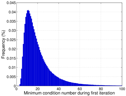
Figure 1: The empirical distribution of miniโก{ฮบโ€‹(Giโ€ โ€‹Gi)}subscript๐‘–๐œ…superscriptsubscript๐บ๐‘–โ€ subscript๐บ๐‘–\min_{i}\{\kappa(G_{i}^{\dagger}G_{i})\} during the first round of recursive decoding.

In Fig.ย 1 we plot the empirical distribution of miniโก{ฮบโ€‹(Giโ€ โ€‹Gi)}subscript๐‘–๐œ…superscriptsubscript๐บ๐‘–โ€ subscript๐บ๐‘–\min_{i}\{\kappa(G_{i}^{\dagger}G_{i})\} averaged over $10^{6}$ channel matrices. As in [5], we notice that the minimal condition number is quite well-behaved, hence it is highly likely that one of the four linear systems in question is well-conditioned and thus we can expect decoding to be successful for a high percentage of channels. In contrast with [5], it is no longer true that the index minimizing the condition number is the one maximizing the determinant. While we are not deciding based solely on the condition number, the index minimizing the condition number is highly correlated with the one maximizing the ratio, having correlation coefficient $\approx 0.6470$.

Refer to caption
Refer to caption
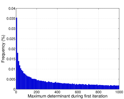
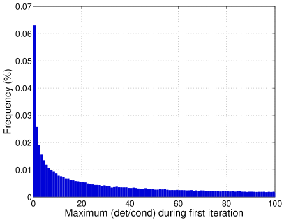
Figure 2: The empirical distributions of maxiโก{det(Giโ€ โ€‹Gi)}subscript๐‘–superscriptsubscript๐บ๐‘–โ€ subscript๐บ๐‘–\max_{i}\{\det(G_{i}^{\dagger}G_{i})\} and maxiโก{det(Giโ€ โ€‹Gi)/ฮบโ€‹(Giโ€ โ€‹Gi)}subscript๐‘–superscriptsubscript๐บ๐‘–โ€ subscript๐บ๐‘–๐œ…superscriptsubscript๐บ๐‘–โ€ subscript๐บ๐‘–\max_{i}\{\det(G_{i}^{\dagger}G_{i})/\kappa(G_{i}^{\dagger}G_{i})\}, respectively, during the first round of recursive decoding.

In Fig.ย 2 we compare the empirical distributions of maxiโก{det(Giโ€ โ€‹Gi)}subscript๐‘–superscriptsubscript๐บ๐‘–โ€ subscript๐บ๐‘–\max_{i}\{\det(G_{i}^{\dagger}G_{i})\} and maxiโก{det(Giโ€ โ€‹Gi)/ฮบโ€‹(Giโ€ โ€‹Gi)}subscript๐‘–superscriptsubscript๐บ๐‘–โ€ subscript๐บ๐‘–๐œ…superscriptsubscript๐บ๐‘–โ€ subscript๐บ๐‘–\max_{i}\{\det(G_{i}^{\dagger}G_{i})/\kappa(G_{i}^{\dagger}G_{i})\}. The similarity of the histograms is a symptom of the high correlation coefficient of $\approx 0.9095$ between the $i$ maximizing the determinant, and that which maximizes the ratio. Thus the decision metric in the algorithm essentially amounts to selecting the index maximizing the determinant, with the condition number selecting the better-conditioned linear system among several with similarly-sized determinants.

6 Conclusions and Future Work

In this article, we have proposed a recursive decoding method for algebraic spaceโ€“time codes of arbitrary size, which has complexity $O(|\mathcal{S}|^{n})$ compared to the worst-case complexity of $O(|\mathcal{S}|^{n^{2}})$ of ML-decoding. The algorithm is based on a decomposition of the representation of the corresponding central simple algebra into a sum of $n$ matrices, each of which encodes $n$ information symbols. These groups of symbols are then decoded recursively, based on certain properties of equivalent channel sub-matrices. As basic examples, we have studied the relevant algebraic decompositions for $2\times 2$ codes and the $4\times 4$ perfect code, as well as provided a first statistical understanding of the algorithm for the latter.

The most immediate task at hand is that of experimental error rates for various algebraic space-time codes, comparing our algorithm with ML-decoding and with the algorithms proposed in [5, 6, 7]. This simulation results are forthcoming and will appear in a later version of this paper. One promising avenue of future work is comparing and possibly combining this approach with that of fast-decodability. The two approaches appear mutually exclusive, and thus could be combined to further reduce decoding complexity.

References

  • [1] Digital Video Broadcasting (DVB): www.dvb.org.
  • [2] Viterbo, E., Boutros, J.: A universal lattice code decoder for fading channel. IEEE Trans. Inf. Theory 45(7) (1999) 1639โ€“1642
  • [3] Biglieri, E., Hong, Y., Viterbo, E.: On fast-decodable spaceโ€“time block codes. IEEE Trans. Inf. Theory 55(2) (2009) 524โ€“530
  • [4] Belfiore, J.C., Rekaya, G., Viterbo, E.: The golden code: a $2\times 2$ full-rate spaceโ€“time code with non-vanishing determinants. IEEE Trans. Inf. Theory 51(4) (2005) 1432โ€“1436
  • [5] Sirinaunpiboon, S., Calderbank, A.R., Howard, S.D.: Fast essentially maximum likelihood decoding of the golden code. IEEE Trans. Inf. Theory 57(6) (2011) 3537โ€“3541
  • [6] Howard, S.D., Sirianunpiboon, S., Calderbank, A.R.: Low complexity essentially maximum likelihood decoding of perfect space-time block codes. In: IEEE International Conference on Acoustics, Speech, and Signal Processing. (2009)
  • [7] Amani, E., Djouani, K., Kurien, A.: Low complexity decoding of the $4\times 4$ perfect spaceโ€“time block code. In: International Conference on Ambient Spaces, Networks and Technologies. (2014)
  • [8] Oggier, F., Belfiore, J.C., Viterbo, E.: Cyclic Division Algebras: A Tool for Space-Time Coding. Volumeย 4 of Foundations and Trends in Communications and Information Theory. Now Publishers (2007)
  • [9] Milne, J.: Class field theory (v4.02) (2013) Available at www.jmilne.org/math/.