Entropic measures of joint uncertainty: effects of lack of majorization

Abstract

We compute Rényi entropies for the statistics of a noisy simultaneous observation of two complementary observables in two-dimensional quantum systems. The relative amount of uncertainty between two states depends on the uncertainty measure used. These results are not reproduced by a more standard duality relation. We show that these behaviors are consistent with the lack of majorization relation between the corresponding statistics.

1 Introduction

Historically, the joint uncertainty of pairs of observables has been mostly addressed in terms of the product of their variances. Nevertheless, there are situations where such formulation is not satisfactory enough [1], thus alternative approaches have been proposed, mainly in terms of diverse entropic measures [2, 3, 4, 5] (see also the reviews in [6]). In this work we consider in particular the so-called Rényi entropies [7] and the corresponding entropic uncertainty relations, for the statistics associated to two complementary observables [8]. There has been an increasing activity to obtain different and improved entropic uncertainty relations not only for foundational reasons but also for the different applications in quantum information problems (a non-exhaustive list includes information-theoretic formulation of error–disturbance relations [9], connection with duality relations [10] and nonlocality [11], entanglement detection [12], EPR-steering inequalities [13], quantum memory [14], and security of quantum cryptography protocols [15]). Also, entropic uncertainty relations have a deep connection with the majorization of statistical distributions [16, 17], which has been already applied to examine uncertainty of thermal states [18] (this is closely related to the idea of mixing character [19]).

However, previous works [4, 8] have shown that entropic uncertainty relations may lead to unexpected results, derived from the fact that the amount of uncertainty for a pair of observables depends on the uncertainty measure used. This is quite natural; actually, one of the benefits of using entropic measures is that they adapt to asses different operational tasks. Nevertheless, one may find it surprising that different measures lead to opposite conclusions in entropic relations: this is, that the states of maximum uncertainty for one measure are the minimum uncertainty states for the other measure, and vice versa.

In this regard, the aim of this work is twofold. On the one hand, we show that these unexpected behaviors are fully compatible with the lack of majorization relation between the corresponding statistics. This connection holds because entropic measures are monotone with respect to majorization. Thus, such surprising entropic results are not tricky features of entropic measures, but may have a deeper meaning that is actually overlooked by more popular measures of uncertainty or complementarity. On the other hand, we extend the application of entropic measures to the statistics of a simultaneous joint observation of two complementary observables in the same system realization [20, 21, 22]. This setting of complementarity in practice provides a rich arena to examine the interplay between entropic measures and majorization. The simultaneous measurement provides a true joint classical-like probability distribution that enables alternative assessments of joint uncertainty, different from the ones given by the product of individual statistics, either intrinsic or of operational origin.

For simplicity we address these issues in the simplest quantum system described by a state in a two-dimensional Hilbert space. This comprises very relevant practical situations such as the path–interference complementarity in two-beam interference experiments. This allows us to contrast the performance of entropic measures with respect to more standard descriptions of complementarity  [23, 24, 25].

The paper is organized as follows: in Sec. 2 we introduce the discussion on statistics of simultaneous measurements for spin $\frac{1}{2}$ observables. Sec. 3 exhibits noticeable results for entropic quantities, and an explanation for that behavior is given in Sec. 4. In Sec. 5, a duality relation for complementarity is analyzed and compared with the entropic results. Finally, some concluding remarks are outlined in Sec. 6.

2 Statistics and simultaneous measurements

Let us consider two complementary observables represented by the Pauli spin matrices $\sigma_{x}$ and $\sigma_{z}$. In practical terms they may represent phase and path, respectively, in two-beam interference experiments. The system state is described by a density matrix operator acting on the Hilbert space ${\cal H}_{S}$ that in Bloch representation acquires the form  $\rho=\frac{1}{2}\left(I+\bm{s}\cdot\bm{\sigma}\right)$, where $I$ is the identity matrix, $\bm{\sigma}$ represents the three Pauli matrices, and $\bm{s}=\mathrm{Tr}(\rho\,\bm{\sigma})$ is a three-dimensional Bloch vector with $|\bm{s}|\leq 1$. The modulus $|\bm{s}|$ expresses the degree of purity of the state as $\mathrm{Tr}(\rho^{2})=\frac{1}{2}(1+|\bm{s}|^{2})$,  being $|\bm{s}|=1$ in the case of a pure state. We make use of the Bloch-sphere parametrization:

$$s_{x}=|\bm{s}|\sin\theta\cos\varphi,\quad s_{y}=|\bm{s}|\sin\theta\sin\varphi,\quad s_{z}=|\bm{s}|\cos\theta.$$ (1)

The intrinsic statistics for the observables $\sigma_{x}$ and $\sigma_{z}$ are

$$p^{X}_{j}=\frac{1}{2}\left(1+j\,s_{x}\right)\textit{\quad}\mbox{and}\quad p^{Z}_{k}=\frac{1}{2}\left(1+k\,s_{z}\right),$$ (2)

with $j=\pm 1$ and $k=\pm 1$.

The simultaneous measurement of noncommuting observables requires involving auxiliary degrees of freedom, usually referred to as apparatus. In our case we consider an apparatus described by a two-dimensional Hilbert space ${\cal H}_{A}$. The measurement performed in ${\cal H}_{A}$ addresses that of $\sigma_{z}$, while $\sigma_{x}$ is measured directly on the system space ${\cal H}_{S}$. The system–apparatus coupling transferring information about $\sigma_{z}$ from the system to the apparatus is arranged via the following unitary transformation acting on ${\cal H}_{S}\otimes{\cal H}_{A}$,

$$U=|+\rangle\langle+|\otimes\ U_{+}+|-\rangle\langle-|\otimes\ U_{-},$$ (3)

where $U_{\pm}$ are unitary operators acting solely on ${\cal H}_{A}$, while $|\pm\rangle$ are the eigenstates of $\sigma_{z}$ with corresponding eigenvalues $\pm 1$. For simplicity the initial state of the apparatus, $|a\rangle\in{\cal H}_{A}$, is assumed to be pure, so that the system–apparatus coupling leads to

$$U|+\rangle|a\rangle\rightarrow\ |+\rangle\ |a_{+}\rangle,\quad U|-\rangle|a\rangle\rightarrow\ |-\rangle\ |a_{-}\rangle,$$ (4)

where the states $|a_{\pm}\rangle=U_{\pm}|a\rangle\in{\cal H}_{A}$ are not orthogonal in general, with $\cos\delta=\langle a_{+}|a_{-}\rangle$ assumed to be a positive real number with $0\leq\delta\leq\pi/2$, without loss of generality. The measurement in ${\cal H}_{A}$ introducing minimum additional noise is given by projection on the orthogonal vectors $|b_{\pm}\rangle$  (see Fig. 1):

$$|b_{+}\rangle = \frac{1}{\cos\phi}\left(\cos\frac{\phi}{2}\,|a_{+}\rangle-\sin\frac{\phi}{2}\,|a_{-}\rangle\right),$$

$$|b_{-}\rangle = \frac{1}{\cos\phi}\left(-\sin\frac{\phi}{2}\,|a_{+}\rangle+\cos\frac{\phi}{2}\,|a_{-}\rangle\right),$$ (5)

where $\phi=\frac{\pi}{2}-\delta$. The added noise is minimum in the sense that the Euclidean distance between $p^{Z}$ and the marginal probability $\tilde{p}^{Z}$ (defined in Eq. (7) below) is minimum [26]. It is worth noting that there is a deep connection of this measurement with the problem of state discrimination between two nonorthogonal states, such as $|a_{\pm}\rangle$ (see e.g. [27]).

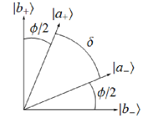
Figure 1: Schematic representation of the states $|a_{\pm}\rangle$ and $|b_{\pm}\rangle$, given in Eqs. (4) and (2) respectively.

The joint statistics for the simultaneous measurement of $\sigma_{x}$ acting on ${\cal H}_{S}$ and of $\sigma_{z}$ addressed by the orthogonal vectors $|b_{\pm}\rangle$ in ${\cal H}_{A}$ is

$$\tilde{p}^{X,Z}_{j,k}=\frac{1}{4}(1+j\,s_{x}\cos\delta+k\,s_{z}\sin\delta),$$ (6)

where $j=\pm 1$ represents the outcomes of the $\sigma_{x}$ measurement, and $k=\pm 1$ those of the $\sigma_{z}$ measurement. The marginal statistics for both observables are

$$\tilde{p}^{X}_{j}=\frac{1}{2}(1+j\,s_{x}\cos\delta)\quad\mbox{and}\quad\tilde{p}^{Z}_{k}=\frac{1}{2}(1+k\,s_{z}\sin\delta).$$ (7)

When contrasted with the intrinsic statistics (2) we get that the observation of $\sigma_{x}$ is exact for $\delta=0$, while the observation of $\sigma_{z}$ is exact for $\delta=\frac{\pi}{2}$. For $\delta=\frac{\pi}{4}$, the extra uncertainty introduced by the unsharp character of the simultaneous observation is balanced between observables.

The expressions given above are valid for any system state $\rho$. However for the sake of simplicity, and given that we focus on the observables $\sigma_{x}$ and $\sigma_{z}$, we will frequently particularize to the set $S$ of states with Bloch vector $\bm{s}$ lying in the $XZ$ plane, this is, for $s_{y}=0$ and $\varphi=0$.

3 Entropic uncertainty assessments

3.1 Rényi entropies and entropic uncertainty relations

We make use of generalized entropies to quantify the uncertainty (or ignorance) related to a probability distribution. Let $p=(p_{1},\ldots,p_{N})$ be the statistics of some observable with $N$ outcomes, then the Rényi entropy [7] of order $\alpha$ reads

$$R_{\alpha}(p)=\frac{1}{1-\alpha}\ln\left(\sum_{i=1}^{N}p_{i}^{\,\alpha}\right),$$ (8)

where $\alpha\geq 0$ is the so-called entropic index. Notice that Shannon entropy [28], $-\sum_{i}p_{i}\ln p_{i}$, is recovered in the limiting case $\alpha\rightarrow 1$. For vanishingly small $\alpha$, one has $R_{0}=\ln||p||_{0}$, where $||p||_{0}$ is the number of nonzero components of the statistics, whereas for arbitrary large $\alpha$, $R_{\infty}=-\ln\max_{i}p_{i}$ only takes into account the greatest component of the statistics and is known as min-entropy, due to the nonincreasing property of $R_{\alpha}$ versus $\alpha$ for a given $p$.

An important property of Rényi entropies is related to majorization (see e.g. [29]). It is said that a statistics $p$ majorizes a statistics $p^{\prime}$, denoted as $p^{\prime}\prec p$, if after forming with $p$ an $N$-dimensional vector with components in decreasing order ($p_{1}\geq p_{2}\geq\ldots\geq p_{N}$) and similarly with $p^{\prime}$, the inequalities   $\sum_{i=1}^{k}p^{\prime}_{i}\leq\sum_{i=1}^{k}p_{i}$  are fulfilled for all $k=1,2,\ldots,N-1$ and $\sum_{i=1}^{N}p^{\prime}_{i}=\sum_{i=1}^{N}p_{i}=1$. Notice that, by definition, the values of $R_{\alpha}$ remains unaltered under rearrangement of the probability vector. The Rényi entropies are order-preserving or Schur-concave functions, this means:

If  $p^{\prime}\prec p$, then  $R_{\alpha}(p^{\prime})\geq R_{\alpha}(p)$ for any $\alpha\geq 0$.

However, majorization is a relation of partial order, so that there are distributions that cannot be compared. We will see that the behaviours that we reporte in the next section are consistent with lack of majorization.

The Schur-concavity property allows to show that Rényi entropies are lower and upper bounded:  since $(\frac{1}{N},\ldots,\frac{1}{N})\prec p\prec(1,0,\ldots,0)$  then, for every $\alpha$, one has  $0\leq R_{\alpha}(p)\leq\ln N$, where the bounds are attained if and only if the corresponding majorization relations reduce to equalities (i.e., for the completely certain situation and the fully random, respectively).

Other relevant property of $R_{\alpha}$ is additivity, that is, for the product of two statistics $p$ and $q$ one has

$$R_{\alpha}(p\,q)=R_{\alpha}(p)+R_{\alpha}(q).$$ (9)

However Rényi entropies do not satisfy, in general, subadditivity and concavity properties .

Following Refs. [8], it can be seen that the Rényi entropic uncertainty relations corresponding to the intrinsic statistics (2) are:

$$R_{\alpha}(p^{X}p^{Z})\geq\left\{\begin{array}[]{ll}\ln 2&\hbox{if }0\leq\alpha\leq\alpha_{I}\\ \frac{2}{1-\alpha}\,\ln\left[\left(\frac{1+\frac{1}{\sqrt{2}}}{2}\right)^{\alpha}+\left(\frac{1-\frac{1}{\sqrt{2}}}{2}\right)^{\alpha}\right]&\hbox{if }\alpha>\alpha_{I},\end{array}\right.$$ (10)

where $\alpha_{I}\approx 1.43$. There are two subsets of states within the set $S$ that compete to be the minimum uncertainty states (as well as those of maximum uncertainty), depending on the value of the entropic index used. We refer to them as extreme and intermediate states:

• Extreme states are eigenstates of $\sigma_{x}$  or  $\sigma_{z}$. These are pure states with $\theta=m\frac{\pi}{2}$ for integer $m$, then $s_{x}=\pm 1,s_{y}=0=s_{z}$,  or  $s_{x}=0=s_{y},s_{z}=\pm 1$. They present full certainty for one observable, and complete uncertainty for the other one.

• Intermediate states are eigenstates of  $\sigma_{x}\pm\sigma_{z}$. These are pure states with $\theta=(2m+1)\frac{\pi}{4}$ for integer $m$, then $s_{x}=\pm s_{z}$, $s_{y}=0$ and $s_{z}=\pm\frac{1}{\sqrt{2}}$. They have essentially the same statistics for both complementary observables so they can be considered as a finite-dimensional counterpart of the Glauber coherent states.

More generally, one has the following mixed versions of extreme and intermediate states, respectively,

$$\rho^{X}_{\mathrm{ex}}=\frac{1}{2}\left(I\pm|\bm{s}|\sigma_{x}\right),\quad\rho^{Z}_{\mathrm{ex}}=\frac{1}{2}\left(I\pm|\bm{s}|\sigma_{z}\right),\quad\rho_{\mathrm{in}}=\frac{1}{2}\left[I\pm\frac{|\bm{s}|}{\sqrt{2}}\left(\sigma_{x}\pm\sigma_{z}\right)\right],$$ (11)

with $|\bm{s}|$ expressing the degree of purity.

3.2 Extreme versus intermediate states

In order to assess the uncertainty related to $\sigma_{x}$ and $\sigma_{z}$, we compute the Rényi entropies of the joint statistics $\tilde{p}^{X,Z}$ (6) and of the product of marginal statistics $\tilde{p}^{X}\tilde{p}^{Z}$ (7), for any given value of the entropic index $\alpha$, as functions of $\theta$ within the set $S$ of states. These quantities are calculated for balanced measurement, $\delta=\frac{\pi}{4}$. We also take into account the Rényi entropies of the product of intrinsic statistics $p^{X}p^{Z}$ (2). For the sake of clarity and to simplify comparisons, we mostly focus on normalized quantities of the form

$$R^{\mathrm{norm}}_{\alpha}(p)=\frac{R_{\alpha}(p)-R_{\alpha,\mathrm{min}}(p)}{R_{\alpha,\mathrm{max}}(p)-R_{\alpha,\mathrm{min}}(p)},$$ (12)

where $R_{\alpha,\mathrm{max}}$ and $R_{\alpha,\mathrm{min}}$ are the maximum and minimum values of $R_{\alpha}$, respectively, within the set $S$.

Figure 2(a) shows $R_{\alpha}^{\mathrm{norm}}(\tilde{p}^{X,Z})$ for $\alpha=1$ and $2.5$ as functions of $\theta$, taking $\varphi=0$ and $|\bm{s}|=1$ for simplicity.

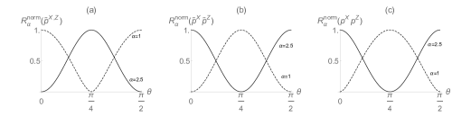
Figure 2: Normalized Rényi entropies (12) of:  (a) the joint statistics $R^{\mathrm{norm}}_{\alpha}(\tilde{p}^{X,Z})$, (b) the product of marginal statistics $R^{\mathrm{norm}}_{\alpha}(\tilde{p}^{X}\tilde{p}^{Z})$, and (c) the product of intrinsic statistics $R^{\mathrm{norm}}_{\alpha}(p^{X}p^{Z})$, for $\alpha=1$ (dashed lines) and $\alpha=2.5$ (solid lines), as functions of $\theta$ for $\varphi=0$, $|\bm{s}|=1$ and $\delta=\frac{\pi}{4}$. The states corresponding to minimal uncertainty vary depending the entropic index used, within each statistical description.

We observe that for $\alpha=1$ the minimum uncertainty states are the intermediate states $\theta=\frac{\pi}{4}$, whereas for $\alpha=2.5$ the minimum uncertainty states are the extreme states $\theta=0$ or $\frac{\pi}{2}$. The opposite happens for the product of marginal statistics $R_{\alpha}(\tilde{p}^{X}\tilde{p}^{Z})$, as illustrated in Fig. 2(b) (that is, for $\alpha=1$ the minimum uncertainty states are the extreme states $\theta=0$ or $\frac{\pi}{2}$, whereas for $\alpha=2.5$ the minimum uncertainty states are the intermediate states $\theta=\frac{\pi}{4}$). The latter result coincides with the conclusions derived from the intrinsic entropies $R_{\alpha}(p^{X}p^{Z})$ as shown in Fig. 2(c) (see also Refs. [8]).

In order to make more explicitly the extreme–intermediate competition for minimum uncertainty, we plot the difference of Rényi entropies between extreme and intermediate states as functions of the entropic index $\alpha$ for $\varphi=0$ and $|\bm{s}|=1$, namely,

$$\Delta R_{\alpha}[p]=R_{\alpha}(p_{\mathrm{ext}})-R_{\alpha}(p_{\mathrm{int}}),$$ (13)

where $p$ stand for the joint, product of marginals, and product of intrinsic statistics, considering balanced measurement $\delta=\frac{\pi}{4}$ (see Fig. 3). $\Delta R_{\alpha}<0$ implies that extreme states are of minimum uncertainty while, on the contrary, $\Delta R_{\alpha}>0$ implies that intermediate states are the minimum uncertainty ones.

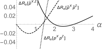
Figure 3: Differences (13) between Rényi entropies for intermediate and extreme states in the cases of joint statistics $\Delta R_{\alpha}[\tilde{p}^{X,Z}]$ (solid line), product of marginals $\Delta R_{\alpha}[\tilde{p}^{X}\tilde{p}^{Z}]$ (dashed line), and the product of intrinsic statistics $\Delta R_{\alpha}[p^{X}p^{Z}]$ (dotted line), as functions of $\alpha$ for $\varphi=0$, $|\bm{s}|=1$, and $\delta=\frac{\pi}{4}$. A negative value of $\Delta R_{\alpha}$ means that extreme states give the minimum uncertainty, whereas a psotive value corresponds to minimizing intermediate states.

We observe that, for the joint statistics, $\Delta R_{\alpha}[\tilde{p}^{X,Z}]$ is negative if $\alpha\in(2,3)$, thus there are two critical values of the entropic index at which the minimizer changes. On the other hand, for the products of marginal and intrinsic statistics, $\Delta R_{\alpha}[\tilde{p}^{X}\tilde{p}^{Z}]$ and $\Delta R_{\alpha}[p^{X}p^{Z}]$ change their sign at one critical value: $\alpha_{M}\approx 1.34$ in the former case and $\alpha_{I}\approx 1.43$ in the latter; in both situations, the difference changes from negative to positive as the entropy index increases.

Let us mention that similar results can be obtained by using the family of Tsallis entropies [32], since there is a one-to-one correspondence between Rényi and Tsallis families of entropies.

4 Majorization assessments

4.1 Extreme and intermediate states are incomparable

Let us call $\tilde{\lambda}=\tilde{p}^{X,Z}_{\textrm{ex}}$ and $\tilde{\mu}=\tilde{p}^{X,Z}_{\textrm{in}}$ the four-dimensional vectors obtained by arranging the values of $\tilde{p}^{X,Z}$ in decreasing order, for extreme and intermediate states, respectively. After Eqs. (6) and (11) we get for $\delta=\pi/4$:

$$\tilde{\lambda}=\frac{1}{4}\left(1+\frac{|\bm{s}|}{\sqrt{2}},1+\frac{|\bm{s}|}{\sqrt{2}},1-\frac{|\bm{s}|}{\sqrt{2}},1-\frac{|\bm{s}|}{\sqrt{2}}\ \right),$$

and

$$\tilde{\mu}=\frac{1}{4}\left(1+|\bm{s}|,1,1,1-|\bm{s}|\right).$$

Thus for all $|\bm{s}|\neq 0$ we have clearly $\tilde{\mu}_{1}>\tilde{\lambda}_{1}$ but $\tilde{\mu}_{1}+\tilde{\mu}_{2}<\tilde{\lambda}_{1}+\tilde{\lambda}_{2}$ so that neither $\tilde{\lambda}\prec\tilde{\mu}$ nor $\tilde{\mu}\prec\tilde{\lambda}$. This shows that contradictions hold for pure as well as for mixed states, while naturally the differences between the extreme and intermediate states are larger for larger $|\bm{s}|$. The lack of majorization is consistent with the change of sign of $\Delta R_{\alpha}[\tilde{p}^{X,Z}]$ reported in Fig. 3 (solid line).

The other behaviors seen in Fig. 3 can be explained in the same way. For the products of marginals $\tilde{p}^{X}\tilde{p}^{Z}$ the four-dimensional ordered vectors for extreme and intermediate states are, after Eqs. (7) and (11), , respectively:

$$\tilde{\lambda}^{\prime}=\tilde{\lambda}$$

and

$$\tilde{\mu}^{\prime}=\frac{1}{4}\left(\left(1+\frac{|\bm{s}|}{2}\right)^{2},1-\frac{|\bm{s}|^{2}}{4},1-\frac{|\bm{s}|^{2}}{4},\left(1-\frac{|\bm{s}|}{2}\right)^{2}\right),$$

for balanced measurement. Thus for all $|\bm{s}|\neq 0$ we have $\tilde{\mu}^{\prime}_{1}>\tilde{\lambda}^{\prime}_{1}$ but $\tilde{\mu}^{\prime}_{1}+\tilde{\mu}^{\prime}_{2}<\tilde{\lambda}^{\prime}_{1}+\tilde{\lambda}^{\prime}_{2}$, so that neither $\tilde{\lambda}^{\prime}\prec\tilde{\mu}^{\prime}$ nor $\tilde{\mu}^{\prime}\prec\tilde{\lambda}^{\prime}$. This correlates with the change of sign of the dashed line in Fig. 3.

The same result is obtained for the comparison of the product of intrinsic statistics $p^{X}p^{Z}$:

$$\lambda=\frac{1}{4}\left(1+|\bm{s}|,1+|\bm{s}|,1-|\bm{s}|,1-|\bm{s}|\right),$$

and

$$\mu=\frac{1}{4}\left(\left(1+\frac{|\bm{s}|}{\sqrt{2}}\right)^{2},1-\frac{|\bm{s}|^{2}}{2},1-\frac{|\bm{s}|^{2}}{2},\left(1-\frac{|\bm{s}|}{\sqrt{2}}\right)^{2}\right),$$

so that for all $|\bm{s}|\neq 0$ we get $\mu_{1}>\lambda_{1}$ but $\mu_{1}+\mu_{2}<\lambda_{1}+\lambda_{2}$. This is consistent with the change of sign of the dotted line in in Fig. 3.

Finally, in the three cases (joint, product of marginals and product of intrinsic statistics) the greatest component of the probability vector for the intermediate state is greater than the corresponding one for the extreme state. Consequently, for sufficiently large $\alpha$ the intermediate states provide the minimum, as seen in the three curves drawn in Fig. 3. However a complete explanation of this figure cannot be provided by the lack of majorization relation.

4.2 Comparison between joint and products of statistics

It is well known that the Rényi entropies do not fulfill in general the subadditivity property. Therefore for the same state the entropy of the joint statistics $\tilde{p}^{X,Z}$ can be larger than the entropy of the product of its marginals $\tilde{p}^{X}\tilde{p}^{Z}$. It can be easily checked that this is actually the case for intermediate states. This behavior implies that $\tilde{p}^{X,Z}$ and $\tilde{p}^{X}\tilde{p}^{Z}$ can not be compared since otherwise subadditivity will follow from Schur-concavity after the case $\alpha=1$ where subadditivity holds.

Nevertheless, one may still wonder whether $\tilde{p}^{X,Z}$ and $p^{X}p^{Z}$ are comparable or not for intermediate states. We can easily show that there are cases for which they are comparable.

In this regard we can begin noting that $\tilde{p}^{X}\prec p^{X}$ and $\tilde{p}^{Z}\prec p^{Z}$, since these statistics are related through a doubly stochastic matrix

$$\pmatrix{\tilde{p}^{X}_{+}\cr\tilde{p}^{X}_{-}}=\pmatrix{\frac{1+\eta}{2}&\frac{1-\eta}{2}\cr\frac{1-\eta}{2}&\frac{1+\eta}{2}}\pmatrix{p^{X}_{+}\cr p^{X}_{-}},$$ (14)

and similarly replacing $X$ by $Z$, where $\eta=\cos\delta,\sin\delta$ for $X,Z$, respectively. Notice that all the matrix entries are positive and that each row and column sums to unity. However this does not imply any trivial relation between $\tilde{p}^{X,Z}$ and $p^{X}p^{Z}$. When comparing the corresponding ordered distributions $\tilde{\mu}$ and $\mu$ for balanced joint measurements, we get $\tilde{\mu}_{1}<\mu_{1}$ as well as $\tilde{\mu}_{1}+\tilde{\mu}_{2}<\mu_{1}+\mu_{2}$ for all $|\bm{s}|\neq 0$. However, we have $\tilde{\mu_{1}}+\tilde{\mu}_{2}+\tilde{\mu}_{3}\leq\mu_{1}+\mu_{2}+\mu_{3}$ for all $|\bm{s}|\leq 2(\sqrt{2}-1)\approx 0.83$, while the opposite holds for $|\bm{s}|$ above this value. This is to say, for intermediate states we get that the natural relation $\tilde{p}^{X,Z}\prec p^{X}p^{Z}$ holds for mixed enough states with $|\bm{s}|\leq 2(\sqrt{2}-1)$, while otherwise the statistics are incomparable.

On the other hand, for extreme states we have always $\tilde{p}^{X,Z}=\tilde{p}^{X}\tilde{p}^{Z}\prec p^{X}p^{Z}$.

4.3 Majorization uncertainty relations

Majorization provides a rather neat form for uncertainty relations in terms of suitable constant vectors that majorize the statistics associated to the observables for every system state [16, 17]. In our case these are

$$\tilde{p}^{X,Z}\prec\tilde{\omega},\quad\tilde{p}^{X}\tilde{p}^{Z}\prec\tilde{\omega}^{\prime}\quad\mbox{and}\quad p^{X}p^{Z}\prec\omega,$$ (15)

where $\tilde{\omega}$, $\tilde{\omega}^{\prime}$, and $\omega$ are constant vectors. By readily applying the procedure outlined in Ref. [17] we obtain

$$\tilde{\omega} = \frac{1}{4}\left(2,\sqrt{2},2-\sqrt{2},0\right),$$

$$\tilde{\omega}^{\prime} = \frac{1}{16\sqrt{2}}\left(9\sqrt{2},8-\sqrt{2},7\sqrt{2}-8,\sqrt{2}\right),$$ (16)

$$\omega = \frac{1}{8}\left(3+2\sqrt{2},5-2\sqrt{2},0,0\right).$$

Then corresponding uncertainty relations hold, for example for the joint distribution one has:  $R_{\alpha}(\tilde{p}^{X,Z})\geq R_{\alpha}(\tilde{\omega})$.

It is worth noting that there is a definite majorization relation between $\omega$ and the other two vectors, that is

$$\tilde{\omega}\prec\omega\quad\mbox{and}\quad\tilde{\omega}^{\prime}\prec\omega.$$ (17)

These two relations are quite natural and express that the uncertainty lower bound is larger for the statistics derived from simultaneous joint measurement, either $\tilde{p}^{X,Z}$ or $\tilde{p}^{X}\tilde{p}^{Z}$, than for the exact intrinsic statistics. This is the majorization relation counterpart of the well-known result that the variance-based lower bound for operational position–momentum uncertainty is at least four times the intrinsic one [20].

However, there is no majorization relation between $\tilde{\omega}$ and $\tilde{\omega}^{\prime}$ since while $\tilde{\omega}_{1}^{\prime}>\tilde{\omega}_{1}$, we have $\tilde{\omega}_{1}^{\prime}+\tilde{\omega}_{2}^{\prime}+\tilde{\omega}_{3}^{\prime}<\tilde{\omega}_{1}+\tilde{\omega}_{2}+\tilde{\omega}_{3}$.

Finally we show that there are no system states leading to statistics equating the distributions (4.3). To this end we use Eqs. (2), (6), and (7) to determine the values of $s_{x}$ and $s_{z}$ that would lead to $\tilde{p}^{X,Z}$, $\tilde{p}^{X}\tilde{p}^{Z}$ and $p^{X}p^{Z}$, equating $\tilde{\omega}$, $\tilde{\omega}^{\prime}$ and $\omega$, respectively. Without loss of generality we consider $s_{x}$ and $s_{z}$ to be positive. For the joint statistics, the null component in $\tilde{\omega}$ implies that $s_{x}=s_{z}=\frac{1}{\sqrt{2}}$. Thus according to (6) the other values for $\tilde{p}^{X,Z}$ should be $\frac{1}{2}$, $\frac{1}{4}$ and $\frac{1}{4}$, which are not equal to the corresponding values in $\tilde{\omega}$. For the product of marginals $\tilde{p}^{X}\tilde{p}^{Z}$, the sum of the greatest and lowest components of $\tilde{\omega}^{\prime}$ imply that $s_{x}=s_{z}=\frac{1}{\sqrt{2}}$. Thus after (7) the other two components for $\tilde{p}^{X}\tilde{p}^{Z}$ should be both $\frac{3}{16}$, which are not equal to the corresponding values in $\tilde{\omega}^{\prime}$. For the intrinsic statistics, we have that the two zeros of $\omega$ imply that either $s_{x}=0$ or $s_{z}=0$. In any case (2) would then imply that the other components of $p^{X}p^{Z}$ should be both $\frac{1}{2}$, which is different from the corresponding values in $\omega$.

5 Duality relation

Following the approach in Ref. [25] we may compare these entropic results with some other assessments of joint uncertainty or complementarity. Among them, one of the most studied is the duality relation between path knowledge and visibility of interference in a Mach–Zehnder interferometric setting [23, 24]. This fits with our approach by regarding $|\pm\rangle$ as representing the internal paths of a Mach–Zehnder interferometer, while $|a_{\pm}\rangle$ represent the states of the apparatus monitoring the path followed by the interfering particle.

One of most used duality expression is [23]

$$D^{2}+V^{2}\leq 1,$$ (18)

where $D=\mathrm{Tr}_{A}\left(\left|w_{+}\rho_{A}^{(+)}-w_{-}\rho_{A}^{(-)}\right|\right)$ is the so-called distinguishability. Regarding the particular case where the system and apparatus are in pure states, we have $\rho_{A}^{(\pm)}=|a_{\pm}\rangle\langle a_{\pm}|$ and $w_{+}=1-w_{-}=\cos^{2}\frac{\theta}{2}$ , so that

$$D=\sqrt{1-4w_{+}w_{-}\left|\langle a_{+}|a_{-}\rangle\right|^{2}}.$$ (19)

This represents the knowledge available about the path followed by the particle, which is grosso modo inversely proportional to path uncertainty. On the other hand, the interference is assessed by the standard fringe visibility $V$ obtained when the relative phase $\varphi$ is varied in Eq. (1),

$$V=2\sqrt{w_{+}w_{-}}\,\left|\langle a_{+}|a_{-}\rangle\right|.$$ (20)

This roughly speaking represents the phase uncertainty, the counterpart of the uncertainty of $\sigma_{x}$ in our approach. Note that in these duality relations path and interference are not treated symmetrically, contrary to the approach developed here in terms of entropic measures.

After Eqs. (19) and (20) we can appreciate that $D^{2}+V^{2}=1$ whenever the system and apparatus are in pure states. This is to say that this duality relation is blind to the differences between extreme and intermediate states, in sharp contrast to the more complete picture provided by the entropic measures with equal entropic indices. This was already shown in Ref. [25] regarding its intrinsic counterpart $P^{2}+V^{2}\leq 1$, where $P=|w_{+}-w_{-}|$ is the predictability. Nevertheless, an equivalence with the duality relation is obtained, using conjugated entropic indices that lead to the so-called min–max entropies, as was recently shown in Ref. [10].

Since the duality relation does not discriminate between pure states it may be interesting to complete the duality analysis by examining the states of maximum $D$ or $V$, as well as those states with $D=V$.

From Eq. (19) the maximum distinguishability, $D=1$, holds either when $w_{+}=0$, $w_{-}=0$, or $\langle a_{+}|a_{-}\rangle=0$. These are all the cases where the particle actually follows just a single path, or when the apparatus can provide full information about the path followed. On the other hand, after Eq. (20), the maximum visibility, $V=|\langle a_{+}|a_{-}\rangle|$, holds when both paths are equally probable $w_{+}=w_{-}=\frac{1}{2}$. Furthermore the maximum visibility reaches unity, $V=1$ when $|a_{+}\rangle$ is proportional to $|a_{-}\rangle$. This is when both paths are equally probable and the apparatus provides no information about the path. Within the set $S$, the extreme states $s_{z}=\pm 1$ satisfy the requirements for extreme distinguishability, while those with $s_{x}=\pm 1$ reach maximum visibility. This agrees with the case of unobserved duality [25].

On the other hand, $D=V$ holds provided that $w_{+}w_{-}\,|\langle a_{+}|a_{-}\rangle|^{2}=\frac{1}{8}$. For balanced detection, $|\langle a_{+}|a_{-}\rangle|=\frac{1}{\sqrt{2}}$ so that $w_{+}w_{-}=\frac{1}{4}$ and then $w_{+}=w_{-}=\frac{1}{2}$. Within the set $S$ this is satisfied by the extreme states being eigenstates of $\sigma_{x}$. Contrary to what happens for the unobserved duality relation, the intermediate states do not satisfy $D=V$. The extreme $s_{x}=\pm 1$ can reach both maximum visibility and $D=V$ since for balanced joint detection we get $D\geq\frac{1}{\sqrt{2}}\geq V$ for all states.

6 Concluding remarks

We have presented several examples of application of Rényi entropies as measures of quantum uncertainty in the case of simultaneous measurements. We have explored those situations leading to unexpected or contradicting predictions for different entropies and states as reported in Sec. 3.2. We have shown that the interplay between extreme and intermediate states as those of minimal uncertainty, shown in Figs. 2 and 3, is consistent with lack of majorization relation between the corresponding statistics, as we have discussed in Sec. 4.1.

Moreover, we have compared the joint and products of statistics in connection with majorization in Sec. 4.2. We have obtained that for the intermediate states, the joint distribution is majorized by the product of intrinsic statistics up to certain degree of purity. On the other hand, for extreme states this situation holds for any degree of purity as naturally one could have expected.

In Sec. 4.3 we have obtained the corresponding majorization uncertainty relations for the joint, product of marginal and product of intrinsic statistics, obtaining the corresponding majorizing constant distributions $\tilde{\omega}$, $\tilde{\omega}^{\prime}$ and $\omega$. We have seen that there exist majorization relations between $\omega$ and $\tilde{\omega}$, and between $\omega$ and $\tilde{\omega}^{\prime}$. This means that the uncertainty lower bound is larger for the statistics derived from simultaneous joint measurement, either $\tilde{p}^{X,Z}$ or $\tilde{p}^{X}\tilde{p}^{Z}$, than for the exact intrinsic statistics. This can be interpreted as the majorization relation counterpart of the well-known result that the variance-based lower bound for operational position–momentum uncertainty is at least four times the intrinsic one. In addition, we have proved that these majorization uncertainty relations are not tight, in the sense that there is no state reaching the bounds.

In Sec.5, we have shown that the new uncertainty relations are much more comprehensive than the traditional assessment of complementarity in terms of distinguishability $D$ and visibility $V$. For a more fruitful comparison we have developed the traditional approach inquiring about the states with extreme $D$ or $V$ , as well as about the intermediate states $D=V$.

The results presented in this work intend to provide a better understanding of uncertainty relations. In recent times there has been a growing interest in applying advanced statistical tools to quantum problems, going beyond the simple use of variances or entropies. Thus, majorization emerges as a powerful tool to understand fundamental aspects of quantum uncertainty and complementarity in the most complete and simple form.

References

- [1] J.M. Lévy-Leblond, Ann. Phys. (N.Y.) 101 (1976) 319–341; E. Breitenberger, Found. Phys. 15 (1985) 353–364; T. Opatrný, J. Phys. A 27 (1994) 7201–7208; G.N. Lawrence, Laser Focus World 30 (1994) 109–114; J. Hilgevoord, Am. J. Phys. 70 (2002) 983–983; J. Řehàček, Z. Hradil, J. Mod. Opt. 51 (2004) 979–982.
- [2] I.I. Hirschman, Am. J. Math. 79 (1957) 152–156; W. Beckner, Ann. Math. 102 (1975) 159- 82; I. Bialynicki-Birula, J. Mycielski, Commun. Math. Phys. 44 (1975) 129–132; D. Deutsch, Phys. Rev. Lett. 50 (1983) 631–633; M. Hossein Partovi, Phys. Rev. Lett. 50 (1983) 1883–1885; K. Kraus, Phys. Rev. D 35 (1987) 3070–3075; H. Maassen, J.B.M. Uffink, Phys. Rev. Lett. 60 (1988) 1103–1106.
- [3] U. Larsen, J. Phys. A 23 (1990) 1041–1061; A.K. Rajagopal, Phys. Lett. A 205 (1995) 32–36; M. Portesi, A. Plastino, Physica A 225 (1996) 412–430; J. Sánchez-Ruiz, Phys. Lett. A 244 (1998) 189–195; I. Bialynicki-Birula, Phys. Rev. A 74 (2006) 052101; J.I. de Vicente, J. Sánchez-Ruiz, Phys. Rev. A 77 (2008) 042110; A.E. Rastegin, J. Phys. A 43 (2011) 155302; G.M. Bosyk, M. Portesi, A. Plastino, S. Zozor, Phys. Rev. A 84 (2011) 056101; M. Jafarpour, A. Sabour, Phys. Rev. A 84 (2011) 032313; G.M. Bosyk, M. Portesi, A. Plastino, Phys. Rev. A 85 (2012) 012108; A.E. Rastegin, Quantum Inf. Process 12 (2013) 2947–2963; Ł. Rudnicki, Z. Puchała, K. Życzkowski, Phys. Rev. A. 89 (2014) 052115; P.J. Coles, M. Piani, Phys. Rev. A 89 (2014) 022112; J. Kaniewski, M. Tomamichel, S. Wehner, Phys. Rev. A 90 (2014) 012332; Ł. Rudnicki, Phys. Rev. A 91 (2015) 032123.
- [4] S. Zozor, M. Portesi, C. Vignat, Physica A 387 (2008) 4800–4808.
- [5] P.A. Bouvrie, J.C. Angulo, J.S. Dehesa, Physica A 390 (2011) 2215–2228; Á. Nagy, E. Romera, Physica A 391 (2012) 3650–3655.
- [6] S. Wehner, A. Winter, New J. Phys. 12 (2010) 025009; I. Bialynicki-Birula, Ł. Rudnicki, in: K.D. Sen (ed.), Statistical Complexity, Springer, Berlin, 2011, Chap. 1.
- [7] A. Rényi, On the measures of entropy and information, Proc. 4th Berkeley Symp. on Mathematics and Statistical Probability, University of California Press, 1961, Vol. 1, pp. 547–561.
- [8] A. Luis, Phys. Rev. A 84 (2011) 034101; S. Zozor, G.M. Bosyk, M. Portesi, J. Phys. A 46 (2013) 465301; S. Zozor, G.M. Bosyk, M. Portesi, J. Phys. A 47 (2014) 495302.
- [9] F. Buscemi, M. J. W. Hall, M. Ozawa, M.M. Wilde, Phys. Rev. Lett. 112 (2014) 050401; P. Mandayam, M.D. Srinivas, Phys. Rev. A 90 (2014) 062128; P.J. Coles, F. Furrer, Phys. lett. A 379 (2015) 105–112; A.E. Rastegin, arXiv:1406.0054v2 (2015).
- [10] P.J. Coles, J. Kaniewski, S. Wehner, Nat. Comm. 5 (2014) 5814.
- [11] M. Tomamichel, E. Hänggi, J. Phys. A: Math. Theor. 46 (2013) 055301.
- [12] V. Giovannetti, Phys. Rev. A 70 (2004) 012102; O. Gühne, M. Lewenstein, Phys. Rev. A 70 (2004) 022316; D.S. Tasca, Ł. Rudnicki, R.M. Gomes, F. Toscano, S. P. Walborn, Phys. Rev. Lett. 110 (2013) 210502.
- [13] S.P. Walborn, A. Salles, R.M. Gomes, F. Toscano, P.H. Souto Ribeiro, Phys. Rev. Lett. 106 (2011) 130402; J. Schneeloch, C.J. Broadbent, S.P. Walborn, E.G. Cavalcanti, J.C. Howell, Phys. Rev. A 87 (2013) 062103; J. Schneeloch, C. J. Broadbent, J. C. Howell, Phys. Lett. A 378 (2014) 766–769 .
- [14] M. Berta, M. Christandl, R. Colbeck, J.M. Renes, R. Renner, Nat. Phys. 6 (2010) 659–662.
- [15] N.H.Y. Ng, M. Berta, S. Wehner, Phys. Rev. A 86 (2012) 042315.
- [16] H. Partovi, Phys. Rev. A 84 (2011) 052117; Z. Puchała, Ł. Rudnicki, K. Życzkowski, J. Phys. A 46 (2013) 272002.
- [17] S. Friedland, V. Gheorghiu, G. Gour, Phys. Rev. Lett. 111 (2013) 230401.
- [18] N. Canosa, R. Rossignoli, M. Portesi, Physica A 368 (2006) 435–441.
- [19] E. Ruch, R. Schranner, T.H. Seligman, J. Chem. Phys. 69 (1978) 386–392; F. Herbut, I. D. Ivanović, J. Phys. A 15 (1982) 1775–1783.
- [20] E. Arthurs, M.S. Goodman, Phys. Rev. Lett. 60 (1988) 2447–2449; S. Stenholm, Ann. Phys. (N.Y.) 218 (1992) 233–254.
- [21] H. Martens, W.M. de Muynck, Found. Phys. 20 (1990) 255–281; H. Martens, W.M. de Muynck, Found. Phys. 20 (1990) 357–380; W.M. de Muynck, H. Martens, Phys. Rev. A 42 (1990) 5079–5085; W.M. de Muynck, J. Phys. A: Math. Gen. 31 (1998) 431–444.
- [22] T. Brougham, E. Andersson, S.M. Barnett, Phys. Rev. A 80 (2009) 042106.
- [23] G. Jaeger, A. Shimony, L. Vaidman, Phys. Rev. A 51 (1995) 54–67; B.-G. Englert, Phys. Rev. Lett. 77 (1996) 2154–2157.
- [24] D.M. Greenberger, A. Yasin, Phys. Lett. A 128 (1988) 391–394; G. Björk, A. Karlsson, Phys. Rev. A 58 (1998) 3477–3483; G. Björk, J. Söderholm, A. Trifonov, T. Tsegaye, A. Karlsson, Phys. Rev. A 60 (1999) 1874–1882; B.-G. Englert, J.A. Bergou, Opt. Commun. 179 (2000) 337–355. P. Busch, C. Shilladay, Phys. Rep. 435 (2006) 1–31; L. Li, N.-L. Liu, S. Yu, Phys. Rev. A 85 (2012) 054101.
- [25] G.M. Bosyk, M. Portesi, F. Holik, A. Plastino, Phys. Scr. 87 (2013) 065002.
- [26] A. Luis, arXiv:1306.5211.
- [27] A. Chefles, Contemp. Phys. 41 (2000) 401–424; M. Dušek, V. Bužek, Phys. Rev. A 66 (2002) 022112; J.A. Bergou, U. Herzog, M. Hillery, Quantum State Estimation (Lecture Notes in Physics vol 649) (Berlin: Springer) (2004) 417–465; J. A. Bergou, V. Bužek, E. Feldman, U. Herzog, M. Hillery, Phys. Rev. A 73 (2006) 062334; J. Bae, L.-C. Kwek, J. Phys. A 48 (2015) 083001.
- [28] C.E. Shannon, Bell Syst. Tech. J. 27 (1948) 623–656 .
- [29] A.W. Marshall, O. Olkin, Inequalities: Theory of Majorization and Its Applications, Academic Press, New York, 1979.
- [30] J. Aczél, Z. Daróczy, in: R. Bellman (ed.), On Measures of Information and Their Characterizations, Academic Press, New York, 1975.
- [31] I. Bengtsson, K. Życzkowski, Geometry of Quantum States: An Introduction to Quantum Entanglement, Cambridge University Press, Cambridge, 2006.
- [32] C. Tsallis, J. Stat. Phys. 52 (1988) 479–487.