On Longest Repeat Queries Using GPU

Abstract

Repeat finding in strings has important applications in subfields such as computational biology. The challenge of finding the longest repeats covering particular string positions was recently proposed and solved by İleri et al., using a total of the optimal $O(n)$ time and space, where $n$ is the string size. However, their solution can only find the leftmost longest repeat for each of the $n$ string position. It is also not known how to parallelize their solution. In this paper, we propose a new solution for longest repeat finding, which although is theoretically suboptimal in time but is conceptually simpler and works faster and uses less memory space in practice than the optimal solution. Further, our solution can find all longest repeats of every string position, while still maintaining a faster processing speed and less memory space usage. Moreover, our solution is parallelizable in the shared memory architecture (SMA), enabling it to take advantage of the modern multi-processor computing platforms such as the general-purpose graphics processing units (GPU). We have implemented both the sequential and parallel versions of our solution. Experiments with both biological and non-biological data show that our sequential and parallel solutions are faster than the optimal solution by a factor of 2–3.5 and 6–14, respectively, and use less memory space.

tring, repeats, longest repeats, parallel computing, GPU, CUDA

1 Introduction

Repetitive structures and regularities finding in genomes and proteins is important as these structures play important roles in the biological functions of genomes and proteins [7, 21, 20, 19, 14, 4, 1, 13]. It is well known that overall about one-third of the whole human genome consists of repeated subsequences [17]; about 10–25% of all known proteins have some form of repetitive structures [14]. In addition, a number of significant problems in molecular sequence analysis can be reduced to repeat finding [16]. Another motivation for finding repeats is to compress the DNA sequences, which is known as one of the most challenging tasks in the data compression field. DNA sequences consist only of symbols from {ACGT} and therefore can be represented by two bits per character. Standard compressors such as gzip and bzip usually use more than two bits per character and therefore cannot achieve good compression. Many modern genomic sequence data compression techniques highly rely on the repeat finding in sequences [15, 2].

The notion of maximal repeat and super maximal repeat [7, 1, 12, 3] captures all the repeats of the whole string in a space-efficient manner, but it does not track the locality of each repeat and thus can not support the finding of repeats that cover a particular string position. For this reason, İleri et al. [8] proposed the challenge of longest repeat query, which is to find the longest repetitive substring(s) that covers a particular string position. Because any substring of a repetitive substring is also repetitive, the solution to longest repeat query effectively provides an effective “stabbing” tool for finding the majority of the repeats covering a string position. İleri et al. proposed an $O(n)$ time and space algorithm that can find the leftmost longest repeat of every string position. Since one has to spend $\Omega(n)$ time and space to read and store the input string, the solution of İleri et al. is optimal.

Our contribution.

In this paper, we propose a new solution for longest repeat query. Although our solution is theoretically suboptimal in the time cost, it is conceptually simpler and runs faster and uses less memory space than the optimal solution in practice. Our solution can also find all longest repeats for every string position while still maintaining a faster processing speed and less space usage, whereas the optimal solution can only find the leftmost candidate. Further, our solution can be parallelized in the shared-memory architecture, enabling it to take advantage of the modern multi-processor computing platforms such as the general-purpose graphics processing units (GPU) [5, 9]. We have implemented both the sequential and parallel versions of our solution. Experiments with both biological and non-biological data show that our solution run faster than the $O(n)$ optimal solution by a factor of 2–3.5 using CPU and 6–14 using GPU, and use less space in both settings.

Road map.

After formulating the problem of longest query in Section 2, we prepare some technical background and observations in Section 3 for our solutions. Section 4 presents the sequential version of our solutions. Following the interpretation in Section 4, it is natural and easy to get the parallel version of our solution, which is presented in Section 5. Section 6 shows the experimental results on the comparison between our solutions and the $O(n)$ solution using real-world data.

2 Problem Formulation

We consider a string $S[1\ldots n]$, where each character $S[i]$ is drawn from an alphabet $\Sigma=\{1,2,\ldots,\sigma\}$. A substring $S[i\ldots j]$ of $S$ represents $S[i]S[i+1]\ldots S[j]$ if $1\leq i\leq j\leq n$, and is an empty string if $i>j$. String $S[i^{\prime}\ldots j^{\prime}]$ is a proper substring of another string $S[i\ldots j]$ if $i\leq i^{\prime}\leq j^{\prime}\leq j$ and $j^{\prime}-i^{\prime}<j-i$. The length of a non-empty substring $S[i\ldots j]$, denoted as $|S[i\ldots j]|$, is $j-i+1$. We define the length of an empty string as zero. A prefix of $S$ is a substring $S[1\ldots i]$ for some $i$, $1\leq i\leq n$. A proper prefix $S[1\ldots i]$ is a prefix of $S$ where $i<n$. A suffix of $S$ is a substring $S[i\ldots n]$ for some $i$, $1\leq i\leq n$. A proper suffix $S[i\ldots n]$ is a suffix of $S$ where $i>1$. We say the character $S[i]$ occupies the string position $i$. We say the substring $S[i\ldots j]$ covers the $k$th position of $S$, if $i\leq k\leq j$. For two strings $A$ and $B$, we write ${\bf A=B}$ (and say $A$ is equal to $B$), if $|A|=|B|$ and $A[i]=B[i]$ for $i=1,2,\ldots,|A|$. We say $A$ is lexicographically smaller than $B$, denoted as ${\bf A<B}$, if (1) $A$ is a proper prefix of $B$, or (2) $A[1]<B[1]$, or (3) there exists an integer $k>1$ such that $A[i]=B[i]$ for all $1\leq i\leq k-1$ but $A[k]<B[k]$. A substring $S[i\ldots j]$ of $S$ is unique, if there does not exist another substring $S[i^{\prime}\ldots j^{\prime}]$ of $S$, such that $S[i\ldots j]=S[i^{\prime}\ldots j^{\prime}]$ but $i\neq i^{\prime}$. A substring is a repeat if it is not unique. A character $S[i]$ is a singleton, if it appears only once in $S$.

Definition 1

For a particular string position $k\in\{1,2,\ldots,n\}$, the longest repeat (LR) covering position ${\bf k}$, denoted as $\operatorname{\mathit{LR}}_{k}$, is a repeat substring $S[i\ldots j]$, such that: (1) $i\leq k\leq j$, and (2) there does not exist another repeat substring $S[i^{\prime}\ldots j^{\prime}]$, such that $i^{\prime}\leq k\leq j^{\prime}$ and $j^{\prime}-i^{\prime}>j-i$.

Obviously, for any string position $k$, if $S[k]$ is not a singleton, $\operatorname{\mathit{LR}}_{k}$ must exist, because at least $S[k]$ itself is a repeat. Further, there might be multiple choices for $\operatorname{\mathit{LR}}_{k}$. For example, if $S={\tt abcabcddbca}$, then $\operatorname{\mathit{LR}}_{2}$ can be either $S[1\ldots 3]={\tt abc}$ or $S[2\ldots 4]={\tt bca}$. In this paper, we study the problem of finding the longest repeats of every string position of $S$.

Problem (longest repeat query): For every string position $k\in\{1,2,\ldots,n\}$, we want to find $\operatorname{\mathit{LR}}_{k}$ or the fact that it does not exist. If multiple choices for $\operatorname{\mathit{LR}}_{k}$ exist, we want to find all of them.

3 Preliminary

The suffix array $\operatorname{\mathit{SA}}[1\ldots n]$ of the string $S$ is a permutation of $\{1,2,\ldots,n\}$, such that for any $i$ and $j$, $1\leq i<j\leq n$, we have $S[\operatorname{\mathit{SA}}[i]\ldots n]<S[\operatorname{\mathit{SA}}[j]\ldots n]$. That is, $\operatorname{\mathit{SA}}[i]$ is the starting position of the $i$th suffix in the sorted order of all the suffixes of $S$. The rank array $\operatorname{\mathit{Rank}}[1\ldots n]$ is the inverse of the suffix array. That is, $\operatorname{\mathit{Rank}}[i]=j$ iff $\operatorname{\mathit{SA}}[j]=i$. The longest common prefix (lcp) array $\operatorname{\mathit{LCP}}[1\ldots n+1]$ is an array of $n+1$ integers, such that for $i=2,3,\ldots,n$, $\operatorname{\mathit{LCP}}[i]$ is the length of the lcp of the two suffixes $S[\operatorname{\mathit{SA}}[i-1]\ldots n]$ and $S[\operatorname{\mathit{SA}}[i]\ldots n]$. We set $\operatorname{\mathit{LCP}}[1]=\operatorname{\mathit{LCP}}[n+1]=0$. In the literature, the lcp array is often defined as an array of $n$ integers. We include an extra zero at $\operatorname{\mathit{LCP}}[n+1]$ is only to simplify the description of our upcoming algorithms. Table 2 shows the suffix array and the lcp array of the example string mississippi.

Definition 2

For a particular string position $k\in\{1,2,\ldots,n\}$, the left-bounded longest repeat (LLR) starting at position $k$, denoted as $\operatorname{\mathit{LLR}}_{k}$, is a repeat $S[k\ldots j]$, such that either $j=n$ or $S[k\ldots j+1]$ is unique.

Clearly, for any string position $k$, if $S[k]$ is not a singleton, $\operatorname{\mathit{LLR}}_{k}$ must exist, because at least $S[k]$ itself is a repeat. Further, if $\operatorname{\mathit{LLR}}_{k}$ does exist, there must be only one choice, because $k$ is a fixed string position and the length of $\operatorname{\mathit{LLR}}_{k}$ must be as long as possible. Lemma 1 shows that, given the rank and lcp arrays of the string $S$, we can directly calculate any $\operatorname{\mathit{LLR}}_{k}$ or find the fact of its nonexistence.

$i$	$\operatorname{\mathit{LCP}}[i]$	$\mathit{\operatorname{\mathit{SA}}}[i]$	suffixes
01	0	110	i
02	1	080	ippi
03	1	050	issippi
04	4	020	ississippi
05	0	010	mississippi
06	0	100	pi
07	1	090	ppi
08	0	070	sippi
09	2	040	sissippi
10	1	060	ssippi
11	3	030	ssissippi
12	0	–	–

Table 1: The suffix array and the lcp array of an example string $S={\tt mississippi}$.

LLR array type	#walk steps	DNA	English	Protein
	Minimum	0000 1	00000 1	0000 1
raw	Maximum	14,836	109,394	25,822
	Average ($=\alpha$)	000 48	004,429	00 215
	Minimum	0000 1	00000 1	0000 1
compact	Maximum	000 14	0000 10	000 35
	Average ($=\beta$)	0000 6	00000 2	0000 3

Table 2: The number of walk steps in the LR’s calculation using our solutions for several $50$MB files from Pizza&Chili 

Lemma 1

For $i=1,2,\ldots,n$:

$$\operatorname{\mathit{LLR}}_{i}=\left\{\begin{array}[]{lll}S[i\ldots i+L_{i}-1]&,&\textrm{\ \ \ if \ \ }L_{i}>0\\ \textit{does not exist}&,&\textrm{\ \ \ if \ \ }L_{i}=0\end{array}\right.$$

where $L_{i}=\max\{\operatorname{\mathit{LCP}}[\operatorname{\mathit{Rank}}[i]],\operatorname{\mathit{LCP}}[\operatorname{\mathit{Rank}}[i]+1]\}$.

Proof

Note that $L_{i}$ is the length of the lcp between the suffix $S[i\ldots n]$ and any other suffix of $S$. If $L_{i}>0$, it means substring $S[i\ldots i+L_{i}-1]$ is the lcp among $S[i\ldots n]$ and any other suffix of $S$. So $S[i\ldots i+L_{i}-1]$ is $\operatorname{\mathit{LLR}}_{i}$. Otherwise ($L_{i}=0$), the letter $S[i]$ is a singleton, so $\operatorname{\mathit{LLR}}_{i}$ does not exist.∎

Clearly, the left-ends of $\operatorname{\mathit{LLR}}_{1},\operatorname{\mathit{LLR}}_{2},\ldots,\operatorname{\mathit{LLR}}_{n}$ strictly increase as $1,2,\ldots,n$. The next lemma shows the right-ends of LLR’s also monotonically increase.

Lemma 2

$|\operatorname{\mathit{LLR}}_{i}|\leq|\operatorname{\mathit{LLR}}_{i+1}|+1$, for every $i=1,2,\ldots,n-1$.

Proof

The claim is obviously correct for the cases when $\operatorname{\mathit{LLR}}_{i}$ does not exist ($|\operatorname{\mathit{LLR}}_{i}|=0$) or $|\operatorname{\mathit{LLR}}_{i}|=1$, so we only consider the case when $|\operatorname{\mathit{LLR}}_{i}|\geq 2$. Suppose $\operatorname{\mathit{LLR}}_{i}=S[i\ldots j]$, $i<j$. It follows that $i+1\leq j$. Since $S[i\ldots j]$ is a repeat, its substring $S[i+1\ldots j]$ is also a repeat. Note that $\operatorname{\mathit{LLR}}_{i+1}$ is the longest repeat substring starting from position $i+1$, so $|\operatorname{\mathit{LLR}}_{i+1}|\geq|S[i+1\ldots j]|=|\operatorname{\mathit{LLR}}_{i}|-1$. ∎

Lemma 3

Every LR is an LLR.

Proof

Assume that $\operatorname{\mathit{LR}}_{k}=S[i\ldots j]$ is not an LLR. Note that $S[i\ldots j]$ is a repeat starting from position $i$. If $S[i\ldots j]$ is not an LLR, it means $S[i\ldots j]$ can be extend to some position $j^{\prime}>j$, so that $S[i\ldots j^{\prime}]$ is still a repeat and also covers position $k$. That says, $|S[i\ldots j^{\prime}]|>|S[i\ldots j]|$. However, the contradiction is that $S[i\ldots j]$ is already the longest repeat covering position $k$. ∎

4 Two Simple and Parallelizable Sequential Algorithms

We know every LR is an LLR (Lemma 3), so the calculation of a particular $\operatorname{\mathit{LR}}_{k}$ is actually a search for the longest one among all LLR’s that cover position $k$. Our discussion starts with the finding of the leftmost LR for every position. In the end, an trivial extension will be made to find all LR’s for every string position.

4.1 Use the raw LLR array

We first calculate $\operatorname{\mathit{LLR}}_{i}$, for $i=1,2,\ldots,n$, using Lemma 1, and save the result in an array $\operatorname{\mathit{LLRr}}[1\ldots n]$, where each $\operatorname{\mathit{LLRr}}[i]=|\operatorname{\mathit{LLR}}_{i}|$. We call $\operatorname{\mathit{LLRr}}[1\ldots n]$ the raw LLR array. Because the rightmost LLR that covers position $k$ is $\operatorname{\mathit{LLR}}_{k}$ and the right boundaries of all LLR’s monotonically increase (Lemma 2), the search for $\operatorname{\mathit{LR}}_{k}$ becomes simply a walk from $\operatorname{\mathit{LLR}}_{k}$ toward the left. The walk will stop when it sees an LLR that does not cover position $k$ or it has reached the left end of the LLRr array. During this walk, we will record the longest LLR that covers position $k$. Ties can be broken by storing the leftmost such LLR. This yields the simple Algorithm 1, which outputs every LR as a $\langle start,length\rangle$ tuple, representing the starting position and the length of the LR.

1

Input: The rank array and the lcp array of the string $S$

2

3

/* Calculate $\operatorname{\mathit{LLR}}_{1},\operatorname{\mathit{LLR}}_{2},\ldots,\operatorname{\mathit{LLR}}_{n}$. */

4

for $i=1,2,\ldots,n$ do  $\operatorname{\mathit{LLRr}}[i]\leftarrow\max\{\operatorname{\mathit{LCP}}[\operatorname{\mathit{Rank}}[i]],\operatorname{\mathit{LCP}}[\operatorname{\mathit{Rank}}[i]+1]\}$;

  // Length of $\operatorname{\mathit{LLR}}_{i}$

5

6;

7

8

/* Calculate $\operatorname{\mathit{LR}}_{1},\operatorname{\mathit{LR}}_{2},\ldots,\operatorname{\mathit{LR}}_{n}$. */

9 for $k=1,2,\ldots,n$ do

10      

      $\operatorname{\mathit{LR}}\leftarrow\langle-1,0\rangle$ ;

        // $\langle start,end\rangle$: start and ending position of $\operatorname{\mathit{LR}}_{k}$.

11      

12      for $i=k$ down to $1$ do

13            

14            if $i+\operatorname{\mathit{LLRr}}[i]-1<k$ then // $\operatorname{\mathit{LLR}}_{i}$ does not exist or does not cover $k$.

                  break;

                    // Early stop

15                  

16            else if $\operatorname{\mathit{LLRr}}[i]\geq\operatorname{\mathit{LR}}.length$ then

17                  $\operatorname{\mathit{LR}}\leftarrow\langle i,\operatorname{\mathit{LLRr}}[i]\rangle$;

18            

19      print $\operatorname{\mathit{LR}}$;

20      

21

22

Algorithm 1 Sequential finding of the leftmost $\operatorname{\mathit{LR}}_{k}$, $k=1,\ldots,n$, using the raw LLR array.

Lemma 4

Given the rank and lcp arrays, Algorithm 1 can find the leftmost $\operatorname{\mathit{LR}}_{k}$ for every $k=1,2,\ldots,n$, using a total of $O(n)$ space and $O(\alpha n)$ time, where $\alpha$ is the average number of LLR’s that cover a string position.

Proof

(1) The time cost for the $\operatorname{\mathit{LLRr}}$ array calculation is obviously $O(n)$. The algorithm finds the LR of each of the $n$ string positions. The average time cost for each LR calculation is bounded by the average number of walk steps, which is equal to the average number of LLR’s that cover a string position. Altogether, the time cost is $O(\alpha n)$. (2) The main memory space is used by the rank, lcp, and $\operatorname{\mathit{LLRr}}$ arrays, each of which has $n$ integers. So altogether the space cost is $O(n)$ words.∎

Theorem 4.1

We can find the leftmost $\operatorname{\mathit{LR}}_{k}$ for every $k=1,2,\ldots,n$, using a total of $O(n)$ space and $O(\alpha n)$ time, where $\alpha$ is the average number of LLR’s that cover a string position.

Proof

The suffix array of $S$ can be constructed using existing $O(n)$-time and space algorithms (For example, [11]). After the suffix array is constructed, the rank array can be trivially created using another $O(n)$ time and space. We can then use the suffix array and the rank array to construct the lcp array using another $O(n)$ time and space [10]. Combining with Lemma 4, the claim in the theorem is proved. ∎

Extension: find all LR’s for every string position.

As we have demonstrated in the example after Definition 1, a particular string position may be covered by multiple LR’s, but Algorithm 1 can only find the leftmost one. However, extending it to find all LR’s for every string position is trivial: During each walk, we simply report all the longest LLR’s that cover the string position, of which we are computing the LR. In order to do so, we will need to do the same walk twice. The first walk is to find the length of the LR and the second walk will actually report all the LR’s. We give the pseudocode of this procedure in Algorithm 3 in the appendix. This algorithm certainly has another extra $O(\alpha)$ time cost on average for each string position’s LR calculation due to the extra walk, but it still gives a total of $O(\alpha n)$ time cost and $O(n)$ space cost.

Corollary 1

We can find all LR’s covering every position $k=1,2,\ldots,n$, using a total of $O(n)$ space and $O(\alpha n)$ time, where $\alpha$ is the average number of LLR’s that cover a string position.

Comment:

(1) Algorithm 1 and 3 are cache friendly. Observe that the finding of every LR essentially is a linear walk over a continuous chunk of the LLRr array. For real-world data, the number of steps in every such walk is quite limited, as shown in the upper rows of Table 1. Note that the English dataset gives a much higher average number of walk steps, because the data was synthesized by appending several real-world English texts together, making many paragraphs appear several times. Because of the few walk steps needed for real-world data, the walking procedure can thus be well cached in the L2 cache, whose size is around several MBs in most nowadays desktops’ CPU architecture, making our algorithm much faster in practice. Note that the optimal $O(n)$ algorithm [8] uses a 2-table system to achieve its optimality, which however has quite a pattern of random accessing the different array locations during its run and thus is not cache friendly. We will demonstrate the comparison with more details in Section 6. (2) Algorithm 1 and 3 are parallelizable in shared-memory architecture. First, each LLR can be calculated independently by a separate thread. After all LLR’s are calculated, each $LR$ can also be calculated independently by a separate thread going through an independent walk. This enables us to implement this algorithm on GPU, which supports massively parallel threads using data parallelism.

4.2 Use the Compact LLR Array

Observe that an LLR can be a substring (suffix, more precisely) of another LLR. For example, suppose $S={\tt ababab}$, then $\operatorname{\mathit{LLR}}_{4}=S[4\ldots 6]={\tt bab}$, which is a substring of $\operatorname{\mathit{LLR}}_{3}=S[3\ldots 6]={\tt abab}$. We know every LR must be an LLR (Lemma 3). So, if an $\operatorname{\mathit{LLR}}_{i}$ is a substring of another $\operatorname{\mathit{LLR}}_{j}$, $\operatorname{\mathit{LLR}}_{i}$ can never be the LR of any string position, because every position covered by $\operatorname{\mathit{LLR}}_{i}$ is also covered by at least another longer LLR, $\operatorname{\mathit{LLR}}_{j}$.

Definition 3

We say an LLR is useless if it is a substring of another LLR; otherwise, it is useful.

Recall that in Algorithm 1 and 3, the calculation of a particular $\operatorname{\mathit{LR}}_{i}$ is a search for the longest one among all LLR’s that cover position $i$. This search procedure is simply a walk from $\operatorname{\mathit{LLR}}_{i}$ toward the left until it sees an LLR that does not cover position $i$ or reaches the left end of the LLRr array. This search can be potentially sped up, if we have had all useless LLR’s eliminated before any search is performed. We will use a new array LLRc, called the compact LLR array, to store all the useful LLR’s in the ascending order of their left ends (as well as of their right ends, automatically).

By Lemma 2, we know if $\operatorname{\mathit{LLR}}_{i-1}$ is not empty, the right boundary of $\operatorname{\mathit{LLR}}_{i}$ is on or after the right boundary of $\operatorname{\mathit{LLR}}_{i-1}$, for any $i\geq 2$. So, we can construct the $\operatorname{\mathit{LLRc}}$ array in one pass as follows. We will calculate every $\operatorname{\mathit{LLR}}_{i}$ using Lemma 1, for $i=1,2,\ldots,n$, and will eliminate every $\operatorname{\mathit{LLR}}_{i}$ if $|\operatorname{\mathit{LLR}}_{i}|=0$ or $|\operatorname{\mathit{LLR}}_{i}|=|\operatorname{\mathit{LLR}}_{i-1}|-1$. Because of the elimination of the useless LLR’s, we will have to save each LLR as a $\langle{\tt start,length}\rangle$ tuple, representing the starting position and the length of the LLR, in the LLRc array. Figure 1 shows the geometric perspective of the elements in an example $\operatorname{\mathit{LLRr}}$ array and its corresponding $\operatorname{\mathit{LLRc}}$ array, where every LLR is represented by a line segment whose start and ending position represent the start and ending position of the LLR.

Note that, in the LLRc array, any two LLR’s share neither the same left-end point (obviously) nor the same right-end point. In other words, the left-end points of all useful LLR’s strictly increase, and so do their right-end points, i.e., all the elements in the LLRc array have been sorted in the strict increasing order of their left-end (as well as right-end) points. See Figure 1(b) for an example. Therefore, given a string position, we will be able to find the leftmost useful LLR that covers that position using a binary search over the LLRc array and the time cost for such a binary search is bounded by $O(\log n)$. After that, we will simply walk along the LLRc array, starting from the LLR returned by the binary search and toward the right. The walk will stop when it sees an LLR that does not cover the string position or it has reached the right end of the LLRc array. During the walk, we will just report the longest LLR that covers the given string position. Ties are broken by picking the leftmost such longest LLR. This leads to the Algorithm 2.

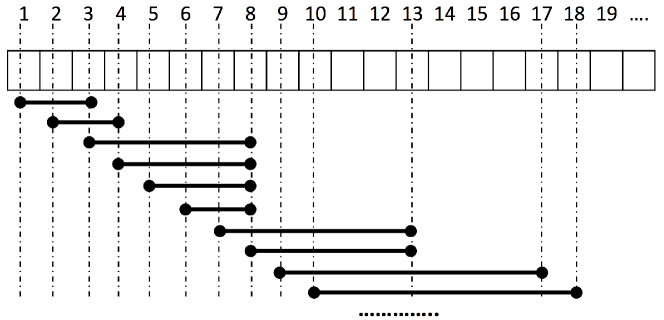
(a) The raw LLR array

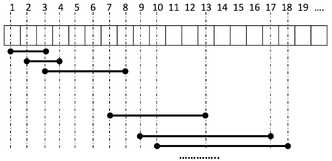
(b) The compact LLR array

Figure 1: The geometric perspective of an example raw LLR array and its corresponding compact LLR array

Lemma 5

Given the rank and lcp arrays, Algorithm 2 can find the leftmost $\operatorname{\mathit{LR}}_{k}$ for every $k=1,2,\ldots,n$, using a total of $O(n)$ space and $O(n(\log n+\beta))$ time, where $\beta$ is the average number of useful LLR’s that cover a string position.

Proof

(1) The time cost for the $\operatorname{\mathit{LLRc}}$ array calculation is obviously $O(n)$ time. The algorithm finds the LR of each of the $n$ string positions. The average time cost for the calculation of the LR of one position includes the $O(\log n)$ time for the binary search and the time cost for the subsequent walk, which is bounded by the average number of useful LLR’s that cover a string position. Altogether, the time cost is $O(n(\log n+\beta))$. (2) The main memory space is used by the rank, lcp, and $\operatorname{\mathit{LLRc}}$ arrays. Each of the rank and lcp arrays has $n$ integers. The $\operatorname{\mathit{LLRc}}$ array has no more than $n$ pairs of integers. Altogether, the space cost $O(n)$ words. ∎

Theorem 4.2

We can find the leftmost $\operatorname{\mathit{LR}}_{k}$ for every $k=1,2,\ldots,n$, using a total of $O(n)$ space and $O(n(\log n+\beta))$ time, where $\beta$ is the average number of useful LLR’s that cover a string position.

Proof

The suffix array of $S$ can be constructed by existing algorithms using $O(n)$ time and space (For example, [11]). After the suffix array is constructed, the rank array can be trivially created using another $O(n)$ time and space. We can then use the suffix array and the rank array to construct the lcp array using another $O(n)$ time and space [10]. Combining the results in Lemma 5, the theorem is proved. ∎

1

Input: The rank array and the lcp array of the string $S$

2

3

/* Calculate the compact LLR array. */

4 $j\leftarrow 1$; $prev\leftarrow 0$;

5

6for $i=1,2,\ldots,n$ do

       $L\leftarrow\max\{\operatorname{\mathit{LCP}}[\operatorname{\mathit{Rank}}[i]],\operatorname{\mathit{LCP}}[\operatorname{\mathit{Rank}}[i]+1]\}$;

        // Length of $\operatorname{\mathit{LLR}}_{i}$

7       if $L>0$ and $L\geq prev$ then  $\operatorname{\mathit{LLRc}}[j]\leftarrow\langle i,L\rangle$; $j\leftarrow j+1$;

8       ;

9       $prev\leftarrow L$;

10      

$size\leftarrow j-1$ ;

  // Size of the $\operatorname{\mathit{LLRc}}$ array.

11

12

/* Calculate $\operatorname{\mathit{LR}}_{1},\operatorname{\mathit{LR}}_{2},\ldots,\operatorname{\mathit{LR}}_{n}$. */

13 for $k=1,2,\ldots,n$ do

14      

      $\operatorname{\mathit{LR}}\leftarrow\langle-1,0\rangle$ ;

        // $\langle start,end\rangle$: start and ending position of $\operatorname{\mathit{LR}}_{k}$.

15      

      $start\leftarrow\textrm{BinarySearch}(\operatorname{\mathit{LLRc}},k)$/* Return the smallest index of the $\operatorname{\mathit{LLRc}}$ array element that covers position $k$, if such element exists; otherwise, return $-1$. */

16      

17      if $start\neq-1$ then

18             for $i=start\ldots size$ do

19                  

20                  if $\operatorname{\mathit{LLRc}}[i].start+\operatorname{\mathit{LLRc}}[i].length-1<k$ then // $\operatorname{\mathit{LLRc}}[i]$ does not cover $k$.

                        break;

                          // Early stop

21                        

22                  else if $\operatorname{\mathit{LLRc}}[i].length>\operatorname{\mathit{LR}}.length$ then

23                        $\operatorname{\mathit{LR}}\leftarrow\operatorname{\mathit{LLRc}}[i]$;

24                  

25            

26      print $\operatorname{\mathit{LR}}$;

27      

28

29

Algorithm 2 Sequential finding of the leftmost $\operatorname{\mathit{LR}}_{k}$, $k=1,\ldots,n$, using the LLRc array.

Extension: find all LR’s for every string position.

Algorithm 2 can also be trivially extended to find all LR’s for every string position by simply reporting all the longest LLR that covers the position during every walk. In order to do so, we will need to walk twice for each string position. The first walk is to get the length of the LR and the second walk will report all the actual LR’s. We give the pseudocode of this procedure in Algorithm 4 in the appendix. This algorithm certainly has another extra $O(\beta)$ time cost on average for each LR’s calculation due to the extra walk, but still gives a total of $O(n(\log n+\beta))$ time cost and $O(n)$ space cost.

Corollary 2

We can find all LR’s of every string position $k=1,2,\ldots,n$, using a total of $O(n)$ space and $O(n(\log n+\beta))$ time, where $\beta$ is the average number of useful LLR’s that cover a string position.

Comment:

(1) The binary searches that are involved in Algorithms 2 and 4 are not cache friendly. However, compared with Algorithms 1 and 3, Algorithms 2 and 4 on average have much fewer steps (the $\beta$ value) in each walk due to the elimination of the useless LLR’s (see the bottom rows of Table 1). This makes Algorithms 2 and 4 much better choices rather than Algorithms 1 and 3 for run environments that have small cache size. Such run environments include the GPU architecture, where the cache size for each thread block is only several KBs. We will demonstrate this claim with more details in Section 6. (2) With more care in the design, Algorithms 2 and 4 are also parallelizable in shared-memory architecture (SMA), which is described in the next Section.

5 Parallel Implementation on GPU

In this section, we describe the GPU version of Algorithms 1 and 2 and their extensions (Algorithms 3 and 4). After we construct the SA, Rank, and LCP arrays on the host CPU , we transfer the Rank array and the LCP array to the GPU device memory. We start with the calculation of the raw LLR array in parallel.

Compute the raw LLR array.

After the LCP and Rank arrays are loaded into GPU memory, we launch a CUDA kernel to compute the raw LLR array on GPU device using massively parallel threads, as illustrated in Figure 2. Each thread $t_{i}$ on the device computes a separate element $\operatorname{\mathit{LLRr}}[i]=|\operatorname{\mathit{LLR}}_{i}|$ using the following equation from Lemma 1.

$$\operatorname{\mathit{LLR}}[i]=\max\{\operatorname{\mathit{LCP}}[\operatorname{\mathit{Rank}}[i],\operatorname{\mathit{LCP}}[\operatorname{\mathit{Rank}}[i]+1]\}$$

Since each $\operatorname{\mathit{LLR}}_{i}$ must start with string position $i$, we only need to save the length of each $\operatorname{\mathit{LLR}}_{i}$ in $\operatorname{\mathit{LLRr}}[i]$. After creating the raw LLR array, we have two options, which in turn lead to two different parallel solutions: using the raw LLR array or the compact LLR array.

5.1 Compute LR’s using the raw LLR array

The parallel implementation of Algorithm 1 using the raw LLR array is straightforward, as presented by the left branch of Figure 2. With the raw LLR array returned from the previous kernel launch on the GPU device, we launch a second kernel for LR calculation. Each CUDA thread $t_{i}$ on the device is to find $\operatorname{\mathit{LR}}_{i}$ by performing a linear walk in the LLRr array, starting at $\operatorname{\mathit{LLRr}}[i]$ toward the left. The walk continues until it finds an LLRr array element that does not cover position $i$ or has reached the left end of the LLRr array. The leftmost or all $\operatorname{\mathit{LR}}_{i}$ can be reported during the walk, as discussed in Algorithm 1. Note that in this search, each CUDA thread checks a chunk of contiguous elements in the LLRr array and this can be cache-efficient.

Taking the calculation of $LR_{10}$ using the raw $\operatorname{\mathit{LLR}}$ array shown in Figure 1(a) as an example. The corresponding CUDA thread $t_{10}$ searches a contiguous chunk of the LLRr array starting from index $10$ down to left in the $\operatorname{\mathit{LLRr}}$ array. We do not search the LLRr elements that are to the right of index $10$, because these elements definitely do not cover position $10$ according to the definition of LLR. In particularly, thread $t_{10}$ goes through $\operatorname{\mathit{LLRr}}[10]$, $\operatorname{\mathit{LLRr}}[9]$, $\operatorname{\mathit{LLRr}}[8]$ and $\operatorname{\mathit{LLRr}}[7]$ to find the longest one among the four of them as $\operatorname{\mathit{LR}}_{10}$. Thread $t_{10}$ stops the search at LLRr position $6$, because $\operatorname{\mathit{LLRr}}[6]$ and all LLR’s to its left do not cover position $10$ (Lemma 2).

Figure 2: Overview of the GPU Implementation

Figure 3: LLR compaction on GPU

5.2 Compute LR’s using the compact LLR array

5.2.1 LLR Compaction.

The right branch of Figure 2 shows the second option in computing LR’s on GPU. That is to use the compact LLR array. We first create the compact LLR array, named as LLRc, from the raw LLR array, which has been created and preserved on the device memory. To avoid the expensive data transfer between the host and the device and to achieve more parallelism, we perform the LLR array compaction on the GPU device in parallel. We launch three CUDA kernels to perform the compaction, denoted as $\mathcal{K}_{1}$, $\mathcal{K}_{2}$, and $\mathcal{K}_{3}$. As shown in Figure 3, after the LLRr array is constructed on the device, we first launch kernel $\mathcal{K}_{1}$ to compute a flag array $Flag[1\ldots n]$ in parallel, where the value of each element $Flag[i]$ is assigned by a separate thread $t_{i}$ as follows: (1) $Flag[1]=1$ iff $\operatorname{\mathit{LLRr}}[1]>0$. (2) $Flag[i]=1$, iff $\operatorname{\mathit{LLRr}}[i]>0$ and $\operatorname{\mathit{LLRr}}[i]\geq\operatorname{\mathit{LLRr}}[i-1]$, for $i=2,3,\ldots,n$. $Flag[i]=0$ means $\operatorname{\mathit{LLR}}_{i}$ is useless and thus can be eliminated.

After the Flag array is constructed from kernel $\mathcal{K}_{1}$, we launch kernel $\mathcal{K}_{2}$ to calculate the prefix sum of the Flag array on the device: $\operatorname{\mathit{Prefix\_Sum}}[i]=\sum_{j=1}^{i}Flag[j]$. We modify the prefix sum function provided by the CUDA toolkit for this purpose.

With the prefix sum array and the Flag array, we launch kernel $\mathcal{K}_{3}$ to copy the useful LLRr array elements into the LLRc array, as illustrated in Figure 3. Each thread $t_{i}$ on the device moves in parallel the $\operatorname{\mathit{LLR}}_{i}$ to an unique destination $\operatorname{\mathit{LLRc}}[\operatorname{\mathit{Prefix\_Sum}}[i]]$, if $Flag[i]=1$. That is, $\operatorname{\mathit{LLRc}}[\operatorname{\mathit{Prefix\_Sum}}[i]]=\langle i,\operatorname{\mathit{LLRr}}[i]\rangle$, if $Flag[i]=1$. Each element in the $\operatorname{\mathit{LLRc}}$ array is a useful LLR and is represented by a tuple of $\langle start,length\rangle$, the start and ending position of the LLR.

5.2.2 Compute LR’s.

After the LLRc array is prepared, we calculate the LR for every string position in parallel. Recall that the calculation of each $\operatorname{\mathit{LR}}_{k}$, for each $k=1,2,\ldots,n$, is a search for the longest useful LLR that covers position $k$. We also know all these relevant LLR’s that we need to search comprise a continuous chunk of the LLRc array. The start position of the chunk can be found using a binary search as we have explained in the discussion of Algorithm 2. After that, a simple linear walk toward the right is performed. The walk continues until it finds an LLRc array element that does not cover position $k$ or has reached the right end of the LLRc array.

To compute the LR’s using the LLRc array, we launch another CUDA kernel, in which each CUDA thread $t_{k}$ first performs a binary search to find the start position of the linear walk and then walk through the relevant LLRc array elements to find either all LR’s or a single LR covering position $k$.

Referring to Figure 1(b), we take the LR calculation covering the string position $9$ as an example. Recall that we have discarded all useless LLR’s in the LLRc array, so the LLRc array element at index $9$ is not necessarily the rightmost LLR that cover string position $9$. Therefore, we have to perform a binary search to locate that leftmost LLRc array element by taking advantage of the nice property of the LLRc array that both the start and ending positions of all LLR’s in it are strictly increasing. After thread $t_{9}$ locates the LLRc element $\operatorname{\mathit{LLRc}}[4]$, the leftmost useful LLR that covers the string position $9$, it performs a linear walk toward the right. The walk will continue until it meets $\operatorname{\mathit{LLRc}}[6]$, which does not cover position $9$. Thread $t_{9}$ will return the longest ones among $\operatorname{\mathit{LLRc}}[4\ldots 6]$ as $\operatorname{\mathit{LR}}_{9}$.

5.3 Advantages and Disadvantages: $\operatorname{\mathit{LLRr}}$ vs. $\operatorname{\mathit{LLRc}}$

When the raw LLR array is used, the algorithm is straightforward and easy to implement, because there is no needs to perform the LLR compaction on the device. However, with a raw LLR array, we could have a large number of useless LLR’s in the raw LLR array, especially when the average length of the longest repeats is quite large. For that reason, the subsequent linear walk for each CUDA thread can take many steps, making the overall search performance worse.

In contrast, under a compact LLR array, we have to perform the LLR compaction, which involves data coping and requires extra memory usage for the $Flag$ and the prefix sum array on the device. In addition, a binary search, which is not present with a raw LLR array, is required to locate the first LLR for the linear walk. The advantage of a compact LLR array is that we remove the useless LLR’s and dramatically shorten the linear walk distance.We provide more analysis and comparison between these two solutions in the experiment section.

6 Experimental Study

Experiment Environment Setup.

We conducted our experiments on a computer running GNU/Linux with a kernel version 3.2.51-1. The computer is equipped with an Intel Xeon 2.40GHz E5-2609 CPU with 10MB Smart Cache and has 16GB RAM. We used a GeForce GTX 660 Ti GPU for our parallel tests. The GPU consists of 1344 CUDA cores and 2GB of RAM memory. The GPU is connected with the host computer with a PCI Express 3.0 interface. We install CUDA toolkit 5.5 on the host computer. We use C to implement our sequential algorithms and use CUDA C to implement our parallel solutions on the GPU, using gcc 4.7.2 with -O3 option and nvcc V5.5.0 as the compilers. We test our algorithms on real-world datasets including biological and non-biological data downloaded from the Pizza&Chili Corpus. The datasets we used are the three $50$MB DNA, English, and Protein pure ASCII text files, each of which thus represents a string of $50\times 1024\times 1024$ characters.

Measurements.

We measured the average time cost of three runs of our program. In order to better highlight the comparison of the algorithmics between the old and our new solutions, we did not include the time cost for the I/O operations that save the results. For the same purpose, we also did not include the time cost for the SA, Rank, and LCP array constructions, because in both the old and our new solutions, these auxiliary data structures are constructed based on the same best suffix array construction code available on the Internet . Our source code for this work is also available on website.

6.1 Time

In the top three charts of Figure 4, using three datasets, we compare different algorithms that return only the leftmost LR for every string position of the input data. In the bottom three charts, we present the performance of our algorithms that are able to find $all$ LR’s for every string position. We compare our new algorithms with the existing optimal sequential algorithm [8], which can only find the leftmost LR for every string position. Table 4 summarizes the speedup of our algorithms against the old optimal algorithm. From experiments, we are able to make the following observations.

Sequential algorithms on CPU.

Our new sequential algorithm using the raw LLR is consistently faster than the old optimal algorithm by a factor of $1.97$–$3.44$, while our new sequential algorithm that uses the compact LLR array is consistently slower. This observation is true in both finding the leftmost LR and all LR’s. (Please note that the old optimal algorithm always finds the leftmost LR only.)

On the host CPU, three dominating factors contribute to the better performance of algorithms using a raw LLR array rather than using a compact LLR array. First, although the compact LLR array can still be constructed in one pass, but the construction involves a lot more computational steps than those needed in the construction of the raw LLR array. Second, sequential algorithms that use a compact LLR array require a binary search in order to locate the starting position of the subsequent linear walk in the calculation of every LR. However, binary searches are not required if we work with a raw LLR array. As it is known, binary search over a large array is not cache friendly. Through profiling, we observe that the binary search operations consume from $63\%$ to $73\%$ of the total execution time. Third, even though for some datasets the search range size (or the number of walk steps) with a raw LLR array could be $10,000$ times larger than that using a compact LLR array, as shown in table 1, the L2 cache ($10$MB) of the host CPU is large enough to cache the range of $contiguous$ LLR’s that each linear walk needs to go through. Such efficient data caching helps all walks take less than a total of 100 milliseconds on the host CPU, accounting for less than $5\%$ of the total execution time, even with the raw LLR array. In other words, given a large cache memory, the number of walk steps is no longer a dominating factor in the overall performance.

Parallel algorithms on GPU.

Our new parallel algorithm on GPU using the compact LLR array is consistently faster than its counterpart that uses the raw LLR array, which is consistently faster than the old optimal algorithm by a factor of $8.32$–$14.62$ in finding the leftmost LR and $6.36$–$10.35$ in finding all LR’s.

Unlike the sequential algorithm on the host CPU, the performance of the parallel algorithm on the GPU device is dominated by the number of LLR’s (the number of walk steps) that each walk will go through. As we profile our GPU implementation, we observe that with the raw LLR array, all linear walks on the GPU take roughly a total of eight seconds for the $English$ dataset. But, the walks take roughly $70$ milliseconds only if using a compact LLR array on the GPU. This is because: (1) the small GPU L2 cache ($384$KB shared by all streaming multiprocessors) cannot host as many LLR’s as what the CPU L2 cache (10MB) can host, resulting in more cache-read misses and more expensive global memory accesses. (2) The number of walk steps with a compact LLR array is less than that with a raw LLR array by a factor of up to four orders of magnitude (see Table 1). (3) The extra time cost for the LLR compaction that is needed when using the compact LLR array become much less significant in the total execution time on GPU. On the host CPU, our sequential solution takes roughly $1.3$ seconds to perform the LLR compaction for datasets of $50$MB and accounts for $20\%$ of the total time cost on average. However, it takes less than $30$ milliseconds on the GPU, accounting for only $9.5\%$ of the entire time cost. We achieve more than $40$ times speedup in the LLR compaction by utilizing GPU device.

The first two reasons above are reassured by the experimental results regarding the English dataset, which we purposely chose to use. The English file is synthesized by simply concatenating several English texts, and thus the text has many repeated paragraphs, which in turn creates many useless LLR’s in the data. In this case, with the raw LLR array, each walk will have a large number of steps due to such useless LLR’s. However, after we compact the raw LLR array, the number of walk steps can be significantly reduced (Table 1) and consequently the GPU code’s performance is significantly improved (Figure 4).

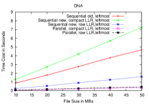
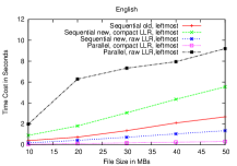
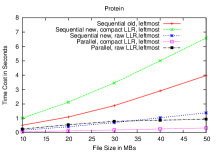
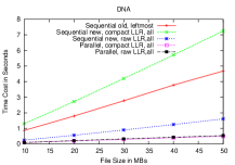
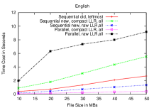
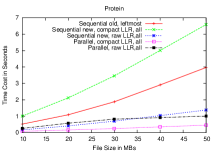
Figure 4: Time Cost vs Dataset Size. The three charts on the top and bottom show the experimental results on finding the leftmost and all repeats of every string position, respectively.

	Sequential	Sequential	Parallel	Parallel
	No Compact	No Compact	Compact	Compact
	Leftmost	All	Leftmost	All
DNA	$2.91$x	$2.91$x	$13.48$x	$\,\ 9.43$x
English	$1.97$x	$1.97$x	$\,\ 8.32$x	$\,\ 6.36$x
Protein	$3.44$x	$3.44$x	$14.62$x	$10.35$x

Table 3: Speedup with 50MB Files

	Old (MBs)	Ours (MBs)	Space Saving
DNA	792.77	650.39	17.96%
English	654.02	650.39	0.56%
Protein	773.53	650.39	15.92%

Table 4: RAM Usage Comparison for 50MB Files

6.2 Space

Table 4 shows the peak memory usage of both the old and our new algorithms for datasets of size $50$MBs. The memory usage of all of our algorithms is the same. This is because the space usage by the SA, Rank, and LCP array dominate the peak memory usage of all of our algorithms. On the other hand, due to its 2-table system that helps achieve the theoretical $O(n)$ time complexity, the old optimal algorithm’s space usage is relevant to the dataset type and is higher than ours.

6.3 Scalability

Although our algorithms have a superlinear time complexity in theory, but they all scale well in practice as shown by Figure 4. As we increase the size of the test data, we observe a consistent speedup. In addition, we did conduct experiments on datasets of 100MB on the GPU device by using a 2D grid of CUDA threads in order to create more than 100 million threads on the device. When finding the leftmost LR for each string position, we observed the same speedups as shown in Figure  4.

On the host CPU, the large cache size dramatically reduces the total number of memory reads during the linear walk in a raw LLR array and thus enables us to eliminate the expensive binary search operations by using a raw LLR array. On the GPU device, although all data is stored in the global memory, a compact LLR array helps greatly reduce the total number of global memory access; each thread linearly searches a smaller number of LLR’s. As shown in Table 1, the average number of walk steps in a compact LLR array is no more than six, which enables the linear walk to be considered as a constant-time operation.

7 Conclusion and Future Work

We proposed conceptually simple and thus easy-to-implement solutions for longest repeat finding over a string. Our algorithm although is not optimal in time theoretically, but runs faster than the old optimal algorithm and uses less space. Further, our algorithm can find all longest repeats of every string position, whereas the old optimal solution can only find the leftmost one. Our algorithm can be parallelized in shared-memory architecture and has been implemented on GPU using the data parallelism to gain further speedup.

Our GPU solution is roughly 4.5 times quicker than our best sequential solution on the CPU, and up to 14.6 times quicker than the old optimal solution on the CPU. Also, we improve the LLR compaction performance by a factor of 40 on GPU. The multiprocessors in our current GPU have a built-in L1 and L2 cache, which help coalesce some global memory accesses. In the future, we will further optimize our parallel solution by utilizing the GPU shared memory or texture memory to further reduce global memory access.

Appendix

1

Input: The rank array and the lcp array of the string $S$

2

3

/* Calculate $\operatorname{\mathit{LLR}}_{1},\operatorname{\mathit{LLR}}_{2},\ldots,\operatorname{\mathit{LLR}}_{n}$. */

4

for $i=1,2,\ldots,n$ do  $\operatorname{\mathit{LLRr}}[i]\leftarrow\max\{\operatorname{\mathit{LCP}}[\operatorname{\mathit{Rank}}[i]],\operatorname{\mathit{LCP}}[\operatorname{\mathit{Rank}}[i]+1]\}$;

  // Length of $\operatorname{\mathit{LLR}}_{i}$

5

6;

7

8

/* Calculate $\operatorname{\mathit{LR}}_{1},\operatorname{\mathit{LR}}_{2},\ldots,\operatorname{\mathit{LR}}_{n}$. */

9 for $k=1,2,\ldots,n$ do

10      

      /* Calculate the length of $\operatorname{\mathit{LR}}_{k}$. */

       $length\leftarrow 0$ ;

        // Length of $\operatorname{\mathit{LR}}_{k}$

11      

12      for $i=k$ down to $1$ do

13            

14            if $i+\operatorname{\mathit{LLRr}}[i]-1<k$ then // $\operatorname{\mathit{LLR}}_{i}$ does not exist or does not cover $k$.

                  break;

                    // Early stop

15                  

16            else if $\operatorname{\mathit{LLRr}}[i]\geq length$ then $length\leftarrow\operatorname{\mathit{LLRr}}[i]$;

17            ;

18            

19      

      /* Calculate all $\operatorname{\mathit{LR}}_{k}$. */

20      

21      if $length>0$ then

22             for $i=k$ down to $1$ do

23                  

24                  if $i+\operatorname{\mathit{LLRr}}[i]-1<k$ then // $\operatorname{\mathit{LLR}}_{i}$ does not exist or does not cover $k$.

                        break;

                          // Early stop

25                        

26                  else if $\operatorname{\mathit{LLRr}}[i]=length$ then

                        print $\langle i,\operatorname{\mathit{LLRr}}[i]\rangle$;

                          // the start and ending positions of $\operatorname{\mathit{LR}}_{k}$

27                        

28                  

29            

30      

      else  print $\langle-1,0\rangle$;

        // $\operatorname{\mathit{LR}}_{k}$ does not exist.

31       ;

32      

33

Algorithm 3 Sequential finding of all $\operatorname{\mathit{LR}}_{k}$ for $k=1,2,\ldots,n$, using the raw LLR array.

1

Input: The rank array and the lcp array of the string $S$

2

3

/* Calculate the compact LLR array. */

4 $j\leftarrow 1$; $prev\leftarrow 0$;

5

6for $i=1,2,\ldots,n$ do

       $L\leftarrow\max\{\operatorname{\mathit{LCP}}[\operatorname{\mathit{Rank}}[i]],\operatorname{\mathit{LCP}}[\operatorname{\mathit{Rank}}[i]+1]\}$;

        // Length of $\operatorname{\mathit{LLR}}_{i}$

7       if $L>0$ and $L\geq prev$ then  $\operatorname{\mathit{LLRc}}[j]\leftarrow\langle i,L\rangle$; $j\leftarrow j+1$;

8       ;

9       $prev\leftarrow L$;

10      

$size\leftarrow j-1$ ;

  // Size of the $\operatorname{\mathit{LLRc}}$ array.

11

12

/* Calculate $\operatorname{\mathit{LR}}_{1},\operatorname{\mathit{LR}}_{2},\ldots,\operatorname{\mathit{LR}}_{n}$. */

13 for $k=1,2,\ldots,n$ do

       $start\leftarrow\textrm{BinarySearch}(\operatorname{\mathit{LLRc}},k)$/* Return the smallest index of the $\operatorname{\mathit{LLRc}}$ array element that covers position $k$, if such element exists; otherwise, return $-1$. */

14      

15      if $start\neq-1$ then

             /* Find the length of $|\operatorname{\mathit{LR}}_{k}|$. */

16             $length\leftarrow 0$;

17            

18            for $i=start\ldots size$ do

19                  

20                  if $\operatorname{\mathit{LLRc}}[i].start+\operatorname{\mathit{LLRc}}[i].length-1<k$ then // $\operatorname{\mathit{LLRc}}[i]$ does not cover $k$.

                        break;

                          // Early stop

21                        

22                  else if $\operatorname{\mathit{LLRc}}[i].length>length$ then $length\leftarrow\operatorname{\mathit{LLRc}}[i].length$;

23                  ;

24                  

            /* Report all $\operatorname{\mathit{LR}}_{k}$. */

25             for $i=start\ldots size$ do

26                  

27                  if $\operatorname{\mathit{LLRc}}[i].start+\operatorname{\mathit{LLRc}}[i].length-1<k$ then // $\operatorname{\mathit{LLRc}}[i]$ does not cover $k$.

                        break;

                          // Early stop

28                        

29                  else if $\operatorname{\mathit{LLRc}}[i].length=length$ then

                        print $\langle\operatorname{\mathit{LLRc}}[i].start,\operatorname{\mathit{LLRc}}[i].length\rangle$ ;

                          // $\langle start,end\rangle$: start and ending pos of $\operatorname{\mathit{LR}}_{k}$.

30                        

31                  

32            

33      else print $\langle-1,0\rangle$;

34      ;

35      

Algorithm 4 Sequential finding of all $\operatorname{\mathit{LR}}_{k}$ for $k=1,\ldots,n$, using the LLRc array.

References

- [1] Becher, V., Deymonnaz, A., Heiber, P.A.: Efficient computation of all perfect repeats in genomic sequences of up to half a gigabyte, with a case study on the human genome. Bioinformatics 25(14), 1746–1753 (2009)
- [2] Behzadi, B., Fessant, F.L.: Dna compression challenge revisited: A dynamic programming approach. In: Annual Symposium on Combinatorial Pattern Matching (2005)
- [3] Beller, T., Berger, K., Ohlebusch, E.: Space-efficient computation of maximal and supermaximal repeats in genome sequences. In: Proceedings of the 19th International Conference on String Processing and Information Retrieval (SPIRE). pp. 99–110 (2012)
- [4] Benson, G.: Tandem repeats finder: a program to analyze dna sequences. Nucleic Acids Research 27(2), 573–580 (1999)
- [5] Che, S., Boyer, M., Meng, J., Tarjan, D., Sheaffer, J., Skadron, K.: A performance study of general-purpose applications on graphics processors using cuda. Journal of Parallel and Distributed Computing 68(10), 1370–1380 (2008)
- [6] Deo, M., Keely, S.: Parallel suffix array and least common prefix for the gpu. In: Proceedings of the 18th ACM SIGPLAN Symposium on Principles and Practice of Parallel Programming (PPoPP). pp. 197–206 (2013)
- [7] Gusfield, D.: Algorithms on strings, trees and sequences: computer science and computational biology. Cambridge University Press (1997)
- [8] İleri, A.M., Külekci, M.O., Xu, B.: On longest repeat queries. http://arxiv.org/abs/1501.06259
- [9] J. Nickolls, J.W., Dally: The gpu computing era. Micro, IEEE 30(2), 56–69 (2010)
- [10] Kasai, T., Lee, G., Arimura, H., Arikawa, S., Park, K.: Linear-time longest-common-prefix computation in suffix arrays and its applications. In: Symposium on Combinatorial Pattern Matching. pp. 181–192 (2001)
- [11] Ko, P., Aluru, S.: Space efficient linear time construction of suffix arrays. Journal of Discrete Algorithms 3(2-4), 143–156 (2005)
- [12] Kulekci, M.O., Vitter, J.S., Xu, B.: Efficient maximal repeat finding using the burrows-wheeler transform and wavelet tree. IEEE Transactions on Computational Biology and Bioinformatics (TCBB) 9(2), 421–429 (2012)
- [13] Kurtz, S., Schleiermacher, C.: Reputer: fast computation of maximal repeats in complete genomes. Bioinformatics 15(5), 426–427 (1999)
- [14] Liu, X., Wang, L.: Finding the region of pseudo-periodic tandem repeats in biological sequences. Algorithms for Molecular Biology 1(1), 2 (2006)
- [15] Manzini, G., Rastero, M.: A simple and fast dna compressor. Software–Practice and Experience 34, 1397–1411 (2004)
- [16] Martinez, H.M.: An efficient method for finding repeats in molecular sequences. Nucleic Acids Research 11(13), 4629–4634 (1983)
- [17] McConkey, E.H.: Human Genetics: The Molecular Revolution. Jones and Bartlett, Boston, MA (1993)
- [18] Osipov, V.: Parallel suffix array construction for shared memory architectures. In: Proceedings of International Symposium on String Processing and Information Retrieval (SPIRE). pp. 379–384 (2012)
- [19] Saha, S., Bridges, S., Magbanua, Z.V., Peterson, D.G.: Computational approaches and tools used in identification of dispersed repetitive dna sequences. Tropical Plant Biology 1(1), 85–96 (2008)
- [20] Saha, S., Bridges, S., Magbanua, Z.V., Peterson, D.G.: Empirical comparison of ab initio repeat finding programs. Nucleic Acids Research 36(7), 2284–2294 (2008)
- [21] Smyth, W.F.: Computing regularities in strings: A survey. European Journal of Combinatorics 34(1), 3–14 (Jan 2013)