Higgs Physics

Abstract

We discuss the interpretation of the LHC Higgs data and the test of the Higgs mechanism. This is done in a more model-independent approach relying on an effective Lagrangian, as well as in specific models like composite Higgs models and supersymmetric extensions of the Standard Model. The proper interpretation of the data requires the inclusion of higher-order corrections both for the relevant Higgs parameters and the production and decay processes. We review recent results obtained within the Collaborative Research Centre / Transregio 9 “Computational Particle Physics”.

1 Introduction

With the announcement of the discovery of a new scalar particle by the LHC experiments ATLAS [1] and CMS [2] particle physics has entered a new era. The discovery immediately triggered activities to study the nature of this particle. The determination of its properties like the spin and parity quantum numbers and the couplings to other Standard Model (SM) particles strongly suggest it to be a Higgs boson, i.e. the particle responsible for electroweak symmetry breaking (EWSB). From the available data, however, it cannot be concluded yet that it is the SM Higgs boson. There is still room for interpretations within numerous extensions beyond the SM (BSM). At the same time, there is no hint for the existence of new particles that might shed light on the true nature of EWSB, which can be weakly or strongly interacting. In view of no direct observation of new states, an effective Lagrangian for the light boson is needed that parametrizes our ignorance of the EWSB sector. Such an effective description is valid as long as New Physics (NP) states appear at a scale much larger than the Higgs boson mass, $M\gg m_{h}$.

At the LHC the Higgs boson couplings cannot be measured without applying model-assumptions. Only ratios of branching ratios, respectively, of couplings are accessible. In order to extract information on the Higgs boson couplings, fits are performed to the experimentally measured values of the signal strengths $\mu$. The signal strengths $\mu$ quantify the Higgs signal rates in a specific final state $X$ with respect to the corresponding SM expectation, and hence are equal to one for the SM Higgs boson. The effective Lagrangian provides a tool that allows to consistently depart from the SM and to calculate BSM rates that can then be used in the fit to the $\mu$ values.

The ultimate step in the experimental verification of the Higgs sector is the measurement of the Higgs self-couplings. With the experimentally extracted self-couplings the Higgs potential can be reconstructed and its typical shape with a non-vanishing vacuum expectation value (VEV) can be tested. While the trilinear Higgs self-coupling is accessible in Higgs pair production, the extraction of the quartic self-interaction from triple Higgs production is beyond the scope of existing and future collider experiments. Due to the smallness of the double Higgs production cross sections and because of large backgrounds the extraction of the trilinear Higgs self-coupling will be challenging and requires highest-possible energies and luminosities.

In this report we will review Higgs boson phenomenology at the LHC. We first investigate in Section 2 a general parametrization of BSM Higgs physics in terms of an effective Lagrangian approach and its implementation into automatic tools for the calculation of Higgs decay rates and production cross sections. Furthermore, its application in fits to the experimentally measured $\mu$ values will briefly be discussed. Section 3 is dedicated to the dominant Higgs pair production processes at the LHC and the higher-order corrections that we have calculated in order to improve the theoretical predictions. We give error estimates for the various processes and present the outcome of a parton level analysis in the gluon fusion process. The next two sections are devoted to Higgs interpretations in BSM models based on strong and weak interaction dynamics. In Section 4 we discuss the phenomenology of composite Higgs models as an example for strong EWSB. Section 5 is devoted to supersymmetric extensions of the Higgs sector, i.e. the minimal (MSSM) and Next-to-Minimal Supersymmetric extension of the SM (NMSSM). The last section 6 closes the review by investigating Higgs coupling measurements at present and future colliders and what can be learned from these with respect to NP extensions beyond the SM.

2 Interpretation of LHC Higgs Data

The effective Lagrangian for the description of NP effects that emerge at scales far beyond the EWSB scale is based on an expansion in the number of fields and derivatives. Its detailed form depends on the assumptions that are applied. In view of the present LHC data it is reasonable to assume the Higgs to be CP-even and part of an $SU(2)_{L}$ doublet as well as baryon- and lepton number conservation. The leading NP effects are then given by 53 operators with dimension 6 [3, 4, 5, 6], considering only one family of quarks and leptons. In case of CP-violation there are another 6 operators. In the strongly-interacting light Higgs (SILH) basis the effective Lagrangian composed of the SM Lagrangian ${\cal L}_{\rm SM}$ and the contributions from dimension-6 operators $O_{i}$ is given by [7, 8]

$${\cal L} = {\cal L}_{\rm SM}+\sum_{i}\bar{c}_{i}O_{i}\equiv{\cal L}_{\rm SM}+\Delta{\cal L}_{\rm SILH}$$ (1)

$$+ \Delta{\cal L}_{F_{1}}+\Delta{\cal L}_{F_{2}}+\Delta{\cal L}_{V}+\Delta{\cal L}_{4F}\,.$$

The explicit form of ${\cal L}_{\text{SM}}$ and the Lagrangians $\Delta{\cal L}_{i}$ containing the dimension-6 operators, along with the conventions for the covariant derivatives and the gauge field strengths can be found in Ref. [9]. The Wilson coefficients $\bar{c}_{i}$ are matrices in flavor space, and a summation over flavor indices has been implicitly assumed. Each of the operators $O_{u,d,l}$ is assumed to be flavor-aligned with the corresponding mass term in order to avoid Flavor-Changing Neutral Currents (FCNC) through the tree-level exchange of the Higgs boson. This leads to the coefficients $\bar{c}_{u,d,l}$ being proportional to the identity matrix in flavor space. Assuming also CP-invariance they are taken to be real. Applying the power counting of Ref. [7], a naive estimate of the Wilson coefficients $\bar{c}_{i}$ has been given in [9]. In the unitary gauge with canonically normalized fields, the SILH effective Lagrangian $\Delta{\cal L}_{\rm SILH}$ can be cast into the form

$${\cal L} = \frac{1}{2}\partial_{\mu}h\ \partial^{\mu}h-\frac{1}{2}m_{h}^{2}h^{2}-c_{3}\,\frac{1}{6}\left(\frac{3m_{h}^{2}}{v}\right)h^{3}$$ (2)

$$- \sum_{\psi=u,d,l}m_{\psi^{(i)}}\,\bar{\psi}^{(i)}\psi^{(i)}\left(1+c_{\psi}\frac{h}{v}+\dots\right)$$

$$+ m_{W}^{2}\,W^{+}_{\mu}W^{-\,\mu}\left(1+2c_{W}\,\frac{h}{v}+\dots\right)$$

$$+ \frac{1}{2}m_{Z}^{2}\,Z_{\mu}Z^{\mu}\left(1+2c_{Z}\,\frac{h}{v}+\dots\right)+\dots$$

$$+ \left(c_{WW}\,W_{\mu\nu}^{+}W^{-\mu\nu}+\frac{c_{ZZ}}{2}\,Z_{\mu\nu}Z^{\mu\nu}+c_{Z\gamma}\,Z_{\mu\nu}\gamma^{\mu\nu}\right.$$

$$\left.+\frac{c_{\gamma\gamma}}{2}\,\gamma_{\mu\nu}\gamma^{\mu\nu}+\frac{c_{gg}}{2}\,G_{\mu\nu}^{a}G^{a\mu\nu}\right)\frac{h}{v}$$

$$+ \Big{(}\left(c_{W\partial W}\,W^{-}_{\nu}D_{\mu}W^{+\mu\nu}+h.c.\right)+c_{Z\partial Z}\,Z_{\nu}\partial_{\mu}Z^{\mu\nu}$$

$$+c_{Z\partial\gamma}\,Z_{\nu}\partial_{\mu}\gamma^{\mu\nu}\Big{)}\,\frac{h}{v}+\dots$$

Shown are terms with up to three fields and at least one Higgs boson. The couplings $c_{i}$ can be expressed as functions linear in the Wilson coefficients of the effective Lagrangian Eq. (1). The explicit relations can be found in Table 1 of Ref. [10]. In particular, as a consequence of the accidental custodial invariance of the SILH Lagrangian at the dimension-6 level [9] the following two relations hold

$$c_{WW}-c_{ZZ}\cos^{2}\!\theta_{W} = c_{Z\gamma}\sin 2\theta_{W}+c_{\gamma\gamma}\sin^{2}\!\theta_{W}$$

$$c_{W\partial W}-c_{Z\partial Z}\cos^{2}\!\theta_{W} = \frac{c_{Z\partial\gamma}}{2}\sin 2\theta_{W}\,.$$ (3)

A third relation, $c_{W}=c_{Z}$, holds if additionally custodial invariance is required for $\Delta{\cal L}_{\rm SILH}$. Allowing for arbitrary values of the couplings $c_{i}$, Eq. (2) is the most general effective Lagrangian at ${\cal O}(p^{4})$ in a derivative expansion by focusing on cubic terms with at least one Higgs boson and making two further assumptions, which are CP conservation and vector fields that couple to conserved currents. The Higgs field in Eq. (2) needs not be part of an electroweak doublet, so that the Lagrangian can be considered as a generalization of $\Delta{\cal L}_{\rm SILH}$. It contains 10 couplings involving a single Higgs boson and two gauge fields ($hVV$ couplings, with $V=W,Z,\gamma,g$), 3 linear combinations of which vanish if custodial symmetry is imposed [9]. If the electroweak (EW) symmetry is realized non-linearly, all Higgs couplings are independent of other parameters not involving the Higgs boson. In a linear realization, however, only 4 $hVV$ couplings are independent of the other EW measurements [11]. Therefore in custodial invariant scenarios it is impossible, by focusing only on $hVV$ couplings, to tell whether the Higgs boson is part of an EW doublet. The doublet nature may be disproved by the decorrelation between the $hVV$ couplings and the other EW data [12, 13, 14, 15].

The parametrizations of BSM couplings in terms of the dimension-6 extension given by $\Delta{\cal L}_{\rm SILH}$ as well as the one given by the non-linear Lagrangian Eq. (2) have been implemented in the Fortran code Ehdecay [10]. Furthermore two benchmark composite Higgs models MCHM₄ [16] and MCHM₅ [17] have been included. It is based on the code Hdecay [18, 19] for the computation of decay widths and branching ratios in the SM and the minimal supersymmetric extension of the SM. All relevant QCD corrections, which generally factorize with respect to the expansion in the number of fields and derivatives of the effective Lagrangian, have been included by using the existing SM computations. The inclusion of the electroweak corrections in a consistent way is only possible in the framework of the SILH Lagrangian and up to higher orders in $(v/f)$. Here $v$ is the weak scale $v\approx 246$ GeV, and $f\equiv M/g_{\star}$ is given in terms of the NP scale $M$ and the typical coupling $g_{\star}$ of the NP sector. In Ehdecay the user can choose to take the EW corrections into account in case of the SILH parametrization.

With the effective Lagrangian Eq. (2) at hand, the $\mu$ rates can be calculated by smoothly departing from the SM in a consistent way. The approach followed here at present [20] is to assume that, while the couplings are modified by an overall modification factor, the coupling structures are not modified with respect to the SM. Furthermore, the narrow width approximation is applied, factorizing the production and decay processes. Finally, the Higgs signal observed at the LHC is supposed to be built up by a single resonance. Our fits performed to the experimentally measured $\mu$ values [22, 23] show that the SM Higgs boson is compatible with the LHC Higgs data within 2$\sigma$. Our fits to a possible invisible branching ratio [23, 24] reveal that large invisible branching ratios are consistent with the LHC measurements.

3 Higgs Pair Production at the LHC

The measurements of the trilinear and quartic Higgs self-couplings allow for the reconstruction of the Higgs potential [25, 26] and thereby the experimental verification of its typical form with a non-vanishing VEV, required for the Higgs mechanism to work. Higgs pair production gives access to the trilinear Higgs self-coupling. The dominant processes for double Higgs production at the LHC are:

• the gluon fusion mechanism $gg\to HH$ [27, 28, 29, 30];

• the $WW/ZZ$ fusion processes (VBF), $qq^{\prime}\to V^{*}V^{*}qq^{\prime}\to HHqq^{\prime}$ ($V=W,Z$) [27, 31, 32, 33, 34];

• the double Higgs-strahlung process, $q\bar{q}^{\prime}\to V^{*}\to VHH$ ($V=W,Z$) [35];

• associated production of two Higgs bosons with a top quark pair, $pp\to t\bar{t}HH$ [36].

The loop-induced gluon fusion process provides the dominant contribution to Higgs pair production. It has been calculated at next-to-leading order (NLO) QCD in an effective field theory (EFT) approximation [30] by applying the low-energy theorem [37, 38, 39], i.e. by assuming infinitely heavy quarks. The NLO cross section for a 125 GeV Higgs boson amounts to $33.89$ fb at a center-of-mass (c.m.) energy of 14 TeV. In obtaining this number the leading order (LO) cross section has been calculated including the full mass dependence in order to improve the perturbative results. The NLO $K$-factor, i.e. the ratio between the NLO and the LO results is large and amounts to 1.5-2 depending on the c.m. energy. The error estimate based on the missing higher order corrections, PDF$+\alpha_{s}$ uncertainties and the application of the EFT approach results in an error of ${\cal O}(30\%)$ at 14 TeV [40]. In the meantime top-quark mass effects at NLO have been estimated [41, 42, 43] and results at next-to-next-to-leading-order (NNLO) in the heavy top mass approximation [44, 45, 46] are available.

The next important di-Higgs production process is vector boson fusion into Higgs pairs, closely followed by Higgs pair production in association with a top-quark pair, which is known at LO QCD only. For the VBF process we have calculated the NLO QCD corrections [40] in the structure function approach in complete analogy to the single Higgs VFB process [47]. Setting the renormalization and factorization scale equal to the momentum of the exchanged weak boson we found an increase of $\sim+7$% of the total cross section with respect to the LO result. For the smallest di-Higgs production process through Higgs-strahlung we have updated the NLO results in analogy to single Higgs-strahlung [48, 49, 50] and computed the QCD corrections at NNLO [40]. At NNLO there is a new gluon-initiated contribution to $ZHH$ production to be taken into account. It turns out that in contrast to single Higgs production [29, 51, 52], its contribution at NNLO is sizeable.

Figure 1 shows the total LHC cross sections for the four classes of Higgs pair production as a function of the c.m. energy. The central renormalization and factorization scales, $\mu_{R}$, respectively, $\mu_{F}$, that have been used are ($\mu_{R}=\mu_{F}=\mu_{0}$)

$$\mu_{0}^{gg\to HH} = M_{HH},\,\,\,\mu_{0}^{qq^{\prime}\to HHqq^{\prime}}=Q_{V^{*}},\,\,\,$$ (4)

$$\mu_{0}^{q\bar{q}^{\prime}\to VHH} = M_{VHH},\,\,\,\mu_{0}^{q\bar{q}/gg\to t\bar{t}HH}=M_{t}\!+\!\frac{1}{2}M_{HH},$$

where $M_{HH}$ denotes the invariant mass of the Higgs pair. Note that all pair production cross sections are $\sim 1000$ times smaller than the corresponding single Higgs production channels. High luminosities are therefore required to probe the Higgs pair production channels at the LHC. The smallness of the cross sections together with the large QCD backgrounds at the LHC make the analysis of di-Higgs production challenging. We have performed a parton-level analysis for the dominant gluon fusion process into Higgs pairs in different final states, which are $b\bar{b}\gamma\gamma$, $b\bar{b}\tau\bar{\tau}$ and $b\bar{b}W^{+}W^{-}$ with the $W$ bosons decaying leptonically. While the $b\bar{b}W^{+}W^{-}$ final state turns out not to be promising after applying acceptance and selection cuts, the significances in the $b\bar{b}\gamma\gamma$ and $b\bar{b}\tau\bar{\tau}$ final states reach $\sim 16$ and $\sim 9$, respectively, after applying the cuts. The event numbers are not too small so that they are promising enough to start a real experimental analysis taking into account detector and hadronization effects. The sensitivity of the various pair production processes to the trilinear Higgs coupling is diluted by additional diagrams to the processes that do not involve the Higgs self-interaction. The sensitivity can be studied by varying the self-coupling in terms of the SM trilinear coupling by a scale factor $\kappa$. The most sensitive channel turns out to be by far the VBF production mode. Taking into account theoretical and statistical uncertainties in the pair production channels the trilinear Higgs self-coupling may be expected to be measured within a factor of two.

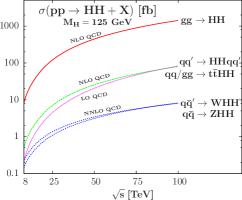
Figure 1: The total cross sections for Higgs pair production at the LHC, including higher order corrections, in the main channels – gluon fusion (red/full), VBF (green/dashed), Higgs-strahlung (blue/dotted), associated production with $t\bar{t}$ (violet/dotted with small dots) – as a function of the c.m. energy with $M_{H}=125$ GeV. The MSTW2008 PDF set has been used and higher order corrections are included. Figure taken from [40] where also details can be found.

4 Composite Higgs Models

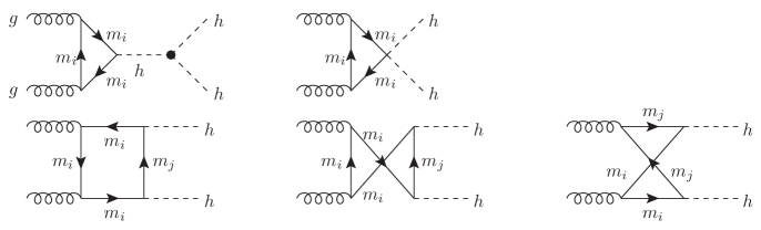
Figure 2: Generic diagrams contributing to double Higgs production via gluon fusion in composite Higgs models with $n_{f}$ novel fermionic resonances of mass $m_{i}$ ($i=1,...,n_{f}$). The index $j$ is introduced to indicate that different fermions can contribute to each box diagram. From Ref. [83].

Composite Higgs Models are examples of models with a strong dynamics underlying EWSB. In these models a light Higgs boson arises as a pseudo Nambu-Goldstone boson from a strongly-interacting sector [53, 54, 55, 56, 57, 58, 59]. This implies modified Higgs couplings with respect to the SM. In Ref. [7] an effective low-energy description of a Strongly Interacting Light Higgs boson has been given, which can be viewed as the first term of an expansion in $\xi=(v/f)^{2}$, with the EWSB scale $v$ and the scale of the strong dynamics $f$. This SILH Lagrangian can be used in the vicinity of the SM limit given by $\xi\to 0$. Larger values of $\xi$ as e.g. the technicolor limit, $\xi\to 1$, require a resummation of the series in $\xi$. This is provided by explicit models built in five-dimensional warped space. In the Minimal Composite Higgs Models (MCHM) of Refs. [16, 17] the global symmetry $SO(5)\times U(1)$ is broken down at the scale $f$ to $SO(4)\times U(1)$ on the infrared brane and to the SM $SU(2)_{L}\times U(1)_{Y}$ on the ultraviolet brane. The modifications of the Higgs couplings in these models can then be described by one single parameter, given by $\xi$. The modification factor of the Higgs coupling to fermions depends on the representations of the bulk symmetry into which the fermions are embedded. In the model of Ref. [16], called $\text{MCHM}_{4}$, the fermions are in the spinorial representation of $SO(5)$, in the model $\text{MCHM}_{5}$ of Ref. [17] they are in the fundamental representation. The question of the generation of fermion masses in composite Higgs models is solved by the hypothesis of partial compositeness [60, 61]. It assumes that the SM fermions, which are elementary, couple linearly to heavy states of the strong sector with the same quantum numbers, implying in particular the top quark to be largely composite. These couplings explicitly break the global symmetry of the strong sector. The Higgs potential is generated from loops of SM particles with EWSB triggered by the top loops which provide the dominant contribution. The Higgs self-couplings therefore also depend on the representation of the fermions, and the Higgs boson mass is related to the fermion sector. It has been shown that a low-mass Higgs boson of $\sim 125$ GeV can naturally be accommodated only if the heavy quark partners are rather light, i.e. for masses below about 1 TeV, see [17, 62, 63, 64, 65, 66, 67]. Phenomenologically the modified Higgs couplings to the SM particles change the Higgs production and decay rates [10, 68]. Another important consequence is the increase of the cross section for double Higgs production in vector boson fusion with the energy [7, 69, 70, 71]. Finally due to the coupling modifications, composite Higgs models are challenged by electroweak precision tests (EWPTs) [7, 72, 73, 74, 75]. The tension with the $S$ and $T$ parameters [76] can be weakened through the contributions from new heavy fermions [77, 78, 79, 80, 81, 82].

So far we do not have any direct evidence for new BSM particles. Indirect information on heavy fermion partners could in principle also be obtained from Higgs physics. These new states would contribute to the loop-induced couplings of the Higgs boson to gluons and photons. It is also these couplings that are involved in the most sensitive Higgs search channels. The structure of these couplings can effectively be described by the Low-Energy Theorem (LET). In [83] we have extended the theorem to take into account possible non-linear Higgs interactions as well as new states resulting from a strong dynamics at the origin of the EWSB. The dominant Higgs production process at the LHC, gluon fusion, is mediated by a top loop with a subleading contribution from the bottom loop. In composite Higgs models with heavy colored fermions and sizable couplings to the Higgs boson, these new states give additional loop contributions that should be taken into account. It has been shown that in explicit constructions gluon fusion into a single Higgs boson, $gg\to h$, computed in the LET approximation, is insensitive to the details of the heavy fermion spectrum [84, 85, 86, 87]. The cross section only depends on the ratio $v/f$, but not on the couplings and the masses of the composite fermions. Although the top Yukawa coupling receives a correction due to the mixing with heavy resonances, which depends on the composite couplings, this contribution is exactly canceled by the loops of the extra fermions, so that the cross section only depends on $v/f$. This holds both in models with partial compositeness and in Little Higgs theories. The gluon fusion cross section in the composite Higgs model can therefore be obtained from the SM result by simply multiplying the latter with the squared rescaling factor of the Yukawa couplings, that comes from the non-linearity of the model. Every correction due to the fermionic resonances can be neglected. This insensitivity to the composite couplings, however, holds exactly only in the LET approximation. There are corrections due to finite fermion mass effects. The LET approximates the gluon fusion Higgs production rate very well, and it indeed turns out that these corrections are very small, even for large values of the compositeness parameter $\xi$.

Another process mediated by colored fermion loops is double Higgs production through gluon fusion. In composite Higgs models the process is changed in two ways compared to the SM. First, there is a genuinely new contribution to the amplitude from a new coupling between two Higgs bosons and two fermions, which arises from the non-linearity of the strong sector. In the SM limit this $f\bar{f}hh$ coupling vanishes. Second, the effects from the top partners in the loop have to be taken into account. They also give rise to a new box diagram that involves off-diagonal Yukawa couplings. These Yukawa couplings only involve the top quark and its charge 2/3 heavy composite partners. The diagrams contributing to the process are shown in Fig. 2. In Ref. [70] a first study on Higgs pair production in composite Higgs models was performed, neglecting top partners. It was found that the cross section can be significantly enhanced due to the new $t\bar{t}hh$ coupling. An explicit calculation of the di-Higgs production cross section in the LET approximation shows that it is insensitive to composite couplings. The reason is a cancellation completely analogous to the single Higgs production case. The comparison with Ref. [70], where the full top mass dependence was retained, shows that the LET underestimates the true result considerably, however.

In the SM it has been known that the $m_{t}\to\infty$ limit approximates the full result only within 20% [30]. Moreover it gives rise to incorrect kinematic distributions [88]. The same is observed in composite Higgs models, and in particular in MCHM₅ the validity of the expansion gets even worse. This behaviour can be understood by looking at the expansion parameter. In single Higgs production this is $m_{h}^{2}/(4m_{t}^{2})$ and the series converges quickly. In double Higgs production, however, the expansion is performed in $\hat{s}/(4m_{t}^{2})$ with the partonic c.m. energy squared $\hat{s}\gg 4m_{h}^{2}$ which is not small, so that the expansion is not as good as in the single Higgs case. In MCHM₅ the presence of the new triangle diagram containing the $t\bar{t}hh$ coupling, which contrary to the triangle diagram with the virtual Higgs boson exchange does not vanish for large $\hat{s}$, renders the convergence of the expansion even worse.

This shall be exemplified for an explicit composite Higgs model, MCHM₅, with extra fermionic resonances. It is based on the symmetry pattern $SO(5)\times U(1)_{X}/SO(4)\times U(1)_{X}$. The additional local symmetry $U(1)_{X}$ is introduced in order to correctly reproduce the fermion charges. The SM electroweak group $SU(2)_{L}\times U(1)_{Y}$ is embedded into $SO(4)\times U(1)_{X}$ and the hypercharge $Y$ is then given by $Y=T_{R}^{3}+X$ [16, 17]. The vector-like fermions introduced in the model have quantum numbers such that they can mix linearly with the SM fermions, the left-handed doublet and right-handed singlet of the third generation $q_{L}=(t_{L},b_{L})^{T}$ and $t_{R}$. At the same time they have ’proto-Yukawa’ interactions with the composite Higgs. The composite fermions are required to transform as a complete ${\bf 5}_{2/3}$ under $SO(5)\times U(1)_{X}$ . In this representation no dangerously large tree-level corrections to the $Zb_{L}b_{L}$ coupling arise, provided a discrete symmetry $P_{LR}$ exchanging the $SU(2)_{L}$ and $SU(2)_{R}$ factors is imposed [17]. Under $SU(2)_{L}\times SU(2)_{R}$ a $\mathbf{5}$ of $SO(5)$ decomposes as $\mathbf{5}\sim(\mathbf{2},\mathbf{2})\oplus(\mathbf{1},\mathbf{1})\,$. The bi-doublet $(\mathbf{2},\mathbf{2})$ is formed by the $SU(2)_{L}$ doublets $Q=(T,B)^{T}$ and $X=(X^{5/3},X^{2/3})^{T}$, while $\tilde{T}$ is a singlet $(\mathbf{1},\mathbf{1})\,$ under $SU(2)_{L}\times SU(2)_{R}$.

The strongest experimental constraints on the model come from the electroweak precision measurements at the $Z$ pole mass at LEP. The modified Higgs couplings to $W$ and $Z$ bosons induce logarithmically divergent contributions to the $S$ and $T$ parameters, which are cut-off by the mass $m_{\rho}$ of the first composite vector resonance [75]. Another BSM effect is the direct contribution of the vector $\rho$ and axial-vector $a$ resonances to the $S$ parameter. Finally the top partners give loop contributions both to the $T$ parameter and the $Zb\bar{b}$ vertex [72, 78, 79, 80]. Figure 3 (left) from Ref. [83] shows the points from a scan over the parameter range of the model after applying a $\chi^{2}$ test, which assesses the agreement of the model with the experimental data. These are the latest EW precision data (EWPD) at that time, and the constraint $|V_{tb}|>0.77$ [89] was applied, which also was the then most up-to-date value. The results are displayed for the left-handed compositeness angle $\phi_{L}$ versus the mass of the lightest top partner, for the compositeness parameter $\xi=0.25$. The constraints on the parameter space from the EWPD can be significantly relaxed by extending the fermion sector of the model [80, 82].

Further constraints are due to flavor physics. In composite Higgs models there arise generically four-fermion operators contributing to flavor-changing (FC) processes and to electric dipole moments. The constraints depend on the exact flavor structure of the model and can be avoided in case of minimal flavor violation (MFV) [90]. While both FC processes and electric dipole moments are inhibited in this case, the MFV assumption requires a large degree of compositeness also for light quarks, so that they have sizeable couplings to the strong sector resonances and lead to a different phenomenology [91]. Dijet searches put constraints on the up and down quarks [92, 93], while the second generation quarks are practically not constrained [94]. An alternative approach is to treat the top quark differently than the light quarks [95]. The flavor bounds can still be satisfied, and since the first two generations are mostly elementary the constraints from EWPT and searches for compositeness are relaxed. In this case both the left-handed and right-handed top can be composite. We do not assume a specific flavor model here. Additional discussions of flavor constraints on composite Higgs models can be found e.g. in Ref. [96].

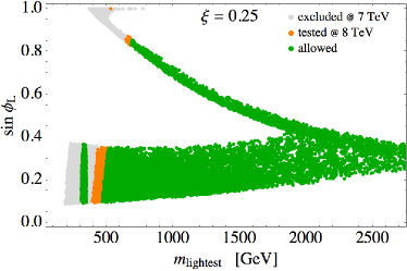
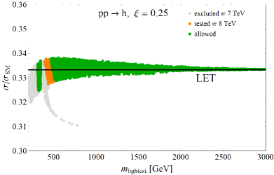
Figure 3: Left: Parameters passing the $\chi^{2}$-test of electroweak precision observables, displaying the compositeness of the left-handed top versus the mass of the lightest top partner, for $\xi=0.25$. Right: The MCHM₅ cross section for single Higgs production through gluon fusion (including the exact dependence on top and heavy fermion masses), normalized to the SM cross section (computed retaining the $m_{t}$ dependence), as a function of the mass of the lightest fermion resonance $m_{\rm{lightest}}$ for $m_{h}=125\,\mathrm{GeV}$ and $\xi=0.25$. The cross section ratio computed with the LET, Eq. (6), is shown as a black line. The points in light grey do not pass the direct collider constraints, points in orange/medium gray pass the 7 TeV constraints but are tested by the LHC running at 8 TeV with an integrated luminosity of $15\,\mathrm{fb}^{-1}$. Figures from Ref. [83].

Another restriction of the model arises from direct searches for new vector-like fermions by ATLAS and CMS. Based on the experimental results from the searches for pair-produced fermions with subsequent decay into the final states $WbWb$, $ZtZt$ and $WtWt$ given in [97, 98, 99], exclusion limits from direct searches have been included in Figure 3 (left). As fermion pair production is a QCD process it only depends on the mass $M_{\psi}$ of the heavy fermion $\psi$. The constraint in a specific final state $X$ then reads,

$$\sigma_{\rm QCD}(pp\to\psi\overline{\psi})\times\mathrm{BR}(\psi\to X)^{2}\leq\sigma_{\rm exp}\,,$$ (5)

where $\sigma_{\rm exp}$ is the upper bound on the cross section, as given by the experiment for each value $M_{\psi}$. The QCD pair production cross sections have been obtained at approximate NNLO [100]. The points that pass the direct search limits from the 7 TeV run are shown in green in Fig. 3 (left). The orange points are tested by LHC8.

The gluon fusion cross section can be computed applying the LET and can be cast into the form

$$\frac{\sigma(pp\to h)}{\sigma(pp\to h)_{\rm SM}}=\left(\frac{1-2\xi}{\sqrt{1-\xi}}\right)^{2}\,.$$ (6)

This result is valid to all orders in $\xi$. It depends purely on the Higgs non-linearities and is independent of the details of the fermion spectrum. When retaining the full mass dependence on the other hand, corrections alter the cross section and are expected to be of the order of at most a few percent. This is confirmed by the full computation of the cross section taking into account the exact dependence on the fermion masses, as can be inferred from Fig. 3 (right).

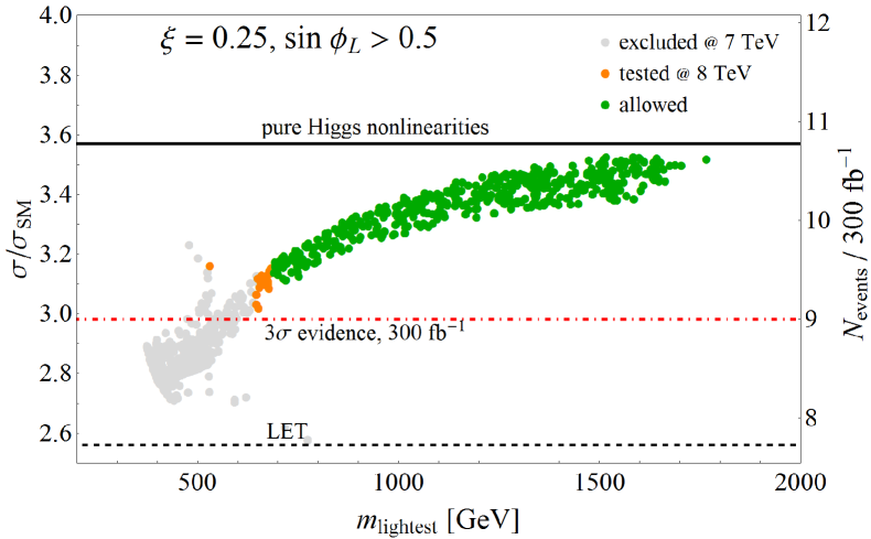
Figure 4: The double Higgs production cross section through gluon fusion normalized to the SM as function of the mass of the lightest heavy top partner, for $m_{h}=125$ GeV and $\xi=0.25$. Green/dark gray (gray) dots denote points which pass (do not pass) the applied constraints, orange/fair gray points are tested by LHC8. The lightest top partner is $X^{2/3}$. The black solid (dashed) line corresponds to the result in the limit of heavy top partners keeping the full top mass dependence (to the LET result). The expected number of events in the $hh\to b\bar{b}\gamma\gamma$ final state after all cuts at LHC14 with $L=300\,\mathrm{fb}^{-1}$ is also shown, along with the $3\sigma$ evidence threshold (dot-dashed line), see Ref. [83].

The figure displays the cross section for single Higgs production through gluon fusion including new fermionic resonances, normalized to the SM cross section with the full top mass dependence, as a function of the mass of the lightest resonance. The QCD $K$-factors, i.e. the ratios between the QCD corrected cross section and the LO result, cancel out under the assumption that the higher order corrections are the same in both cases. In green are shown the points that pass the EWPTs, gray and orange points do not satisfy the collider bounds. The agreement between the full result and the prediction using the low-energy theorem, shown by the black line, confirms that the cross section for single Higgs production is almost independent of the details of the spectrum and is fixed only by the value of $\xi$. For heavy fermion partners the sensitivity to the composite couplings practically vanishes. The LET hence provides a very accurate cross section for single Higgs production for any spectrum of the heavy fermions. The figure furthermore shows that in the MCHM5 single Higgs production is suppressed compared to the SM for $\xi=0.25$. This can be understood from the LET result given in Eq. (6).

Applying the LET to double Higgs production results in the partonic cross section

$$\hat{\sigma}_{gg\to hh}=\frac{G_{F}^{2}\alpha_{s}^{2}(\mu)\hat{s}}{128(2\pi)^{3}}\,\frac{1}{9}\,\sqrt{1-\frac{4m_{h}^{2}}{\hat{s}}}\,C_{\textrm{LET}}^{2}(\hat{s})\;,$$ (7)

where $G_{F}$ denotes the Fermi constant and $\alpha_{s}$ the strong coupling constant evaluated at the scale $\mu$. The amplitude in the limit of heavy loop particle masses at all orders in $\xi$ is given by

$$C^{\scriptsize\mbox{LET}}_{\rm MCHM5}(\hat{s})=\frac{3m_{h}^{2}}{\hat{s}-m_{h}^{2}}\left(\frac{1-2\xi}{\sqrt{1-\xi}}\right)^{2}-\frac{1}{1-\xi}\;.$$ (8)

As in single Higgs production the LET cross section for Higgs pair production is insensitive to the details of the heavy fermion spectrum and fixed uniquely by $\xi$. In contrast to single Higgs production, for Higgs pair production the cross section is enhanced compared to the SM. In the SM Higgs pairs are produced through Higgs bosons coupling to gluons via triangle loops and boxes. The related amplitudes interfere destructively. In the MCHM5 the two contributions are modified by $((1-\xi)/\sqrt{1-\xi})^{2}$, and there is an additional diagram with the two-Higgs two-fermion coupling proportional to $\xi$, which can hence have order one effects and thus govern the total cross section.

Figure 4 shows the double Higgs production process normalized to the SM cross section as a function of the lightest top partner mass. The points result from a scan over the parameter range of the model. In the computation of the cross sections the full mass dependence of the loop particles has been taken into account. In the black solid line the full mass dependence on the top quark mass has been kept while the heavy fermion partners have been integrated out. The dashed line displays the result in the LET approximation, i.e. sending all loop particle masses to infinity. The color code is the same as in Fig. 3. The figure shows that there is a sizeable dependence of the cross section on the spectrum of the heavy fermions. We have $2.7\raisebox{-3.69899pt}{~{}\shortstack{$<$ \\ [-0.07cm] $\sim$}}~{}\sigma/\sigma_{\rm SM}\raisebox{-3.69899pt}{~{}\shortstack{$<$ \\ [-0.07cm] $\sim$}}~{}3.7$. The LET cross section and the one in the limit of heavy partners on the other hand only depend on $\xi$. However, the LET approximation considerably underestimates the full result. Note that in the figure the cross section is consistently normalized to the SM result for $m_{t}\to\infty$. The result in the limit of heavy partners and keeping the full top mass dependence on the other hand, overestimates the cross section for masses of the lightest fermion partner below about 1 TeV. This is the region that is compatible with a 125 GeV Higgs boson. For larger masses of the fermion partners, the cross section approaches the result retaining only the top-loop contribution, as expected. Higher-order QCD corrections have not been taken into account in the figure. Due to the additional two-Higgs two-fermion diagram and the box diagram with different loop particle masses they cannot be taken over from the SM. For heavy loop particle masses the corrections should not be too different from the SM case though, so that they approximately cancel out in the ratio of the cross sections.

So far we have only treated the case of composite top quarks. With the bottom quark being the next-heaviest quark a sizeable mixing with the strong sector can be expected also for the bottom quark. Due to the small bottom mass, the LET cannot be applied any more and the loop-induced Higgs couplings to gluons are expected to depend on the resonance structure of the strong sector, with significant implications for the Higgs phenomenology [82, 86, 91]. The effects of composite bottom quarks on composite Higgs models and the LHC Higgs phenomenology can be studied by embedding the fermions in the 10. This is the smallest possible representation of $SO(5)$ that allows to include partial compositeness for the bottom quarks and at the same time is compatible with EWPTs by implementing custodial symmetry. The bottom quark mass is in this case not introduced at hoc any more but generated through the mixing with the strong sector. The 10 leads to a larger spectrum of new heavy fermions compared to the previous case with composite top quarks only. The new vector-like fermions transform under the $SU(2)_{L}\times SU(2)_{R}$ and are given by $u$, $u_{1}$, $t_{4}$ and $T_{4}$ with electric charge 2/3, $d$, $d_{1}$ and $d_{4}$ with charge -1/3 and finally $\chi$, $\chi_{1}$ and $\chi_{4}$ with charge 5/3. The model is strongly constrained by EWPTs, in particular there are one-loop contributions to the non-oblique corrections to the $Zb_{L}\bar{b}_{L}$ vertex due to the partial compositeness of the bottom quark. This coupling has been measured very precisely and agrees with the SM prediction at the sub-percent level. It is safe from large corrections for the fermion embedding in the 10 representation, where $b_{L}$ belongs to a bi-doublet of $SU(2)_{L}\times SU(2)_{R}$ and the $SO(4)$ is enlarged to $O(4)$. The general formulae for the contributions of new bottom partners in the loop corrections to $Zb_{L}b_{L}$ have been derived in [82] and can be applied to other models with similar particle content. In order to test the viability of the model a scan over its parameter space has been performed, setting the top and bottom quark masses to $m_{t}=173.2$ GeV and $m_{b}=4.2$ GeV, respectively, and the Higgs boson mass to $m_{h}=125$ GeV. A $\chi^{2}$ test is performed including the constraints from EWPD, and only those points have been retained that also fulfil $|V_{tb}|>0.92$ [101]. The result is shown in Fig. 5 in the $\Delta\chi^{2}\equiv\chi^{2}-\chi^{2}_{\rm min}$ versus $\xi$ plane. The smallest $\Delta\chi^{2}$ values are obtained for $0.01<\xi<0.2$. High $\xi$ values lead to large $\Delta\chi^{2}$, corresponding to a compatibility with EWPTs at 99% confidence level (C.L.). The positive fermionic contributions to the $T$ parameter play an important role here for the compatibility as they drive back the $T$ value into the region in accordance with the EW precision data.

Figure 5: Parameters passing the $\chi^{2}$ test of electroweak precision observables, fulfilling in addition $|V_{tb}|>0.92$, for a scan over the parameter space. Details can be found in Ref. [82]. Dark blue: $68\%$ C.L. region, medium blue: $95\%$ C.L. region and light blue: $99\%$ C.L. region, in the $\Delta\chi^{2}$ versus $\xi$ plane.

	$|V_{tb}|>0.92$			$|V_{tb}|$ in $\chi^{2}$
Experiment	$\xi$	$\chi^{2}/n$	$\chi^{2}_{n}$	$\xi$	$\chi^{2}/n$	$\chi^{2}_{n}$
ATLAS	0.105	8.06/9	0.90	0.096	12.34/10	1.23
	0.0	17.54/13	1.35	0.0	17.73/14	1.25
CMS	0.057	5.22/10	0.52	0.055	6.36/11	0.58
	0.0	9.90/14	0.71	0.0	10.09/15	0.67

Table 1: Global $\chi^{2}$ results for the best fit point taking into account EWPT and the Higgs results for ATLAS and CMS, respectively: Left: For parameter points which fulfil $|V_{tb}|>0.92$. Right: When including the measured value of $|V_{tb}|$ in the $\chi^{2}$ test. The lines for $\xi=0.0$ list for comparison the SM values. The number of degrees of freedom $n$ are counted naively as the difference between the number of observables and the number of parameters in the model, and $\chi^{2}_{n}\equiv\chi^{2}/n$. Table from [82].

The SM limit is obtained for $\xi\to 0$ and $M_{10}\to\infty$, where $M_{10}$ sets the scale for the top and bottom partner masses. Due to the restriction of the scan to $M_{10}\leq 10$ TeV it is not contained in the plot.

The LHC Higgs search data put further constraints on the model. The inclusion of heavy bottom and top quarks leads to changes in the Higgs Yukawa couplings and new heavy fermions in the loop-induced production and decay processes. In particular, in contrast to the heavy top partner case, in the dominant gluon fusion production process due to the mixing with bottom partners the LET cannot be applied any more, so that the cross section now depends on the details of the model. Also the compatibility with the direct searches for new vector-like fermions performed by ATLAS [102] and CMS [103, 104] has to be tested. Flavor physics further constrains the model. As this depends on the exact flavor structure of the model which is not specified here, these constraints are not taken into account in this investigation. For a random scan over the parameter range a $\chi^{2}$ test is performed taking into account EWPTs, Higgs data and the experimental results on $V_{tb}$. The results from direct fermion searches are taken into account by discarding all points that lead to masses below the exclusion limits. In Table 1 the $\chi^{2}$ values of the best fit points are reported together with those for the SM for comparison. The constraint from $V_{tb}$ has been included in two different ways. Either all points with $|V_{tb}|>0.92$ are rejected or the best fit value given by the experiments is included in the $\chi^{2}$ test. The global $\chi^{2}$ is increased when including $V_{tb}$, in particular in the composite Higgs model. The table shows that the CMS [105] data are better described than the ATLAS data [106]. The best fit points are obtained for $\xi\approx 0.1$ for ATLAS and for $\xi\approx 0.05$ for CMS. In the composite Higgs model their $\chi^{2}$ is slightly smaller than in the SM, due to the larger number of free parameters. An estimate of the relative goodness of the fit is given by $\chi^{2}_{n}\equiv\chi^{2}/n$, where $n$ denotes the number of degrees of freedom.

Our discussion shows that composite Higgs models, although challenged by constraints from EWPTs, flavor physics, direct searches for new fermions and the light Higgs mass, are still viable extensions beyond the SM Higgs. They provide an explanation of EWSB based on strong dynamics and hence an alternative to weakly coupled models as e.g. supersymmetry, which shall be discussed in the following.

5 Supersymmetric Higgs Models

Supersymmetric theories [107, 108, 109, 110, 111, 112, 113, 114, 115, 116, 117, 118, 119, 120, 121] provide a natural solution to the hierarchy problem by introducing a new symmetry between fermionic and bosonic degrees of freedom. They are among the most extensively studied BSM extensions. In order to ensure supersymmetry (SUSY) and an anomaly-free theory two complex Higgs doublets have to be introduced, $H_{u}$ to provide masses to the up-type fermions, and $H_{d}$ to ensure masses for the down-type fermions. In sections 5.1 and 5.2 we will discuss Higgs physics in two popular supersymmetric models, the minimal (MSSM) [122] and next-to-minimal supersymmetric model (NMSSM) [123], respectively.

5.1 Associated heavy quark Higgs production in the MSSM

After electroweak symmetry breaking, three of the eight degrees of freedom contained in $H_{u}$ and $H_{d}$ are absorbed by the $Z$ and $W$ gauge bosons, leaving five elementary Higgs particles in the MSSM. These consist of two CP-even neutral (scalar) particles $h,H$, one CP-odd neutral (pseudoscalar) particle $A$, and two charged bosons $H^{\pm}$. At leading order the MSSM Higgs sector is fixed by two independent input parameters which are usually chosen as the pseudoscalar Higgs mass $M_{A}$ and $\tan\beta=v_{u}/v_{d}$, the ratio of the vacuum expectation values of $H_{u}$ and $H_{d}$, respectively. Including the one-loop and dominant two-loop corrections the upper bound of the light scalar Higgs mass is $M_{h}\raisebox{-3.69899pt}{~{}\shortstack{$<$ \\ [-0.07cm] $\sim$}}~{}135$ GeV [124] for supersymmetric mass scales up to about a TeV.

An important property of the bottom Yukawa couplings is their enhancement for large values of $\tan\beta$. The top Yukawa couplings, on the other hand, are suppressed for large $\tan\beta$ [125], unless the light (heavy) scalar Higgs mass is close to its upper (lower) bound, where their couplings become SM-like. The couplings of the various neutral MSSM Higgs bosons to fermions and gauge bosons, normalized to the SM Higgs couplings, are listed in Table 2, where the angle $\alpha$ denotes the mixing angle of the scalar Higgs bosons $h,H$.

$\phi$		$g^{\phi}_{u}$	$g^{\phi}_{d}$	$g^{\phi}_{V}$
SM	$H$	1	1	1
MSSM	$h$	$\cos\alpha/\sin\beta$	$-\sin\alpha/\cos\beta$	$\sin(\beta-\alpha)$
	$H$	$\sin\alpha/\sin\beta$	$\cos\alpha/\cos\beta$	$\cos(\beta-\alpha)$
	$A$	$1/\tan\beta$	$\tan\beta$	0

Table 2: MSSM Higgs couplings to $u$- and $d$-type fermions and gauge bosons [$V=W,Z$] relative to the SM couplings.

The negative direct searches for neutral MSSM Higgs bosons at LEP2 have lead to lower bounds of $M_{h,H}>92.8$ GeV and $M_{A}>93.4$ GeV [126]. The LEP2 results also exclude the range $0.7<\tan\beta<2.0$ in the MSSM, assuming a SUSY scale $M_{\rm SUSY}=1$ TeV [126]. MSSM Higgs-boson searches have continued at the $p\bar{p}$ collider Tevatron, see e.g. [127], and form the central part of the current and future physics program of the LHC [128]. The present LHC searches at 7 and 8 TeV c.m. energy have excluded parts of the MSSM parameter space for large values of $\tan\beta$ [129]. However, the recent discovery of a resonance with a mass near 125 GeV [1, 2] is a clear indication for the existence of a SM or beyond-the-SM Higgs boson. While the properties of the new particle, as determined so far, are consistent with those predicted within the SM, the bosonic state at 125 GeV can also be interpreted as a supersymmetric Higgs boson.

Neutral MSSM Higgs boson production at the LHC is dominated by gluon fusion, $gg\to h/H/A$, and by the associated production of a Higgs boson with bottom quarks. Gluon fusion is most significant at small and moderate $\tan\beta$. At large values of $\tan\beta$, however, bottom–Higgs associated production

$$q\bar{q}/gg\to b\bar{b}+h/H/A$$ (9)

constitutes the dominant Higgs-boson production process. Here, we shall focus on precision calculations for bottom–Higgs associated production at the LHC. We refer the reader to Refs. [130, 131, 132] and references therein for a discussion of higher-order calculations for gluon fusion.

The NLO QCD corrections to Higgs-bottom associated production, Eq. (9), can be inferred from the analogous calculation involving top quarks [133, 134]. However, they turn out to be numerically enhanced [135] by large logarithmic contributions from the phase space region with final-state bottom quarks at small small transverse momenta. Those logarithms can be resummed by introducing bottom-quark densities in the proton [136] and by applying the standard DGLAP evolution. In this so-called five-flavor scheme (5FS) the leading-order process is [137]

$$b\bar{b}\to h/H/A\,,$$

where the transverse momenta of the incoming bottom quarks, their masses, and their off-shellness are neglected at LO. The NLO [138] and NNLO [139] QCD corrections as well as the SUSY–electroweak corrections [140] to these bottom-initiated processes have been calculated. They are of moderate size, if the running bottom Yukawa coupling is introduced at the scale of the corresponding Higgs-boson mass. The fully exclusive $gg\to b\bar{b}+h/H/A$ process, calculated with four active parton flavors in a four-flavor scheme (4FS), and the 5FS calculation converge at higher perturbative orders, and there is fair numerical agreement between the NLO 4FS and NNLO 5FS cross section predictions [130, 131, 135, 141]. In Ref. [142] a scheme has been proposed to match the 4FS and 5FS cross sections (“Santander matching”). The scheme is based on the observation that the 4FS and 5FS calculations of the cross section are better motivated in the asymptotic limits of small and large Higgs masses, respectively, and combines the two approaches in such a way that they are given variable weight, depending on the value of the Higgs-boson mass.

If both bottom jets accompanying the Higgs boson in the final state are tagged, one has to rely on the fully exclusive calculation for $gg\to b\bar{b}+h/H/A$. For the case of a single $b$-tag in the final state the corresponding calculation in the 5FS starts from the process $bg\to b+h/H/A$ with the final-state bottom quark carrying finite transverse momentum. The NLO QCD, electroweak, and NLO SUSY-QCD corrections to this process have been calculated [143].

State-of-the-art predictions as well as estimates of the corresponding parametric and theoretical uncertainties have been provided by the LHC Higgs Cross Section Working Group both for total [130] and differential [131, 132] cross sections.

Recently, the 4FS calculations for heavy quark plus Higgs associated production at the LHC have been improved by including the full SUSY-QCD corrections within the MSSM and separating the dominating universal part in terms of effective Yukawa couplings [144]. The SUSY loop corrections modify the tree-level relation between the bottom mass and its Yukawa coupling, which is enhanced at large $\tan\beta$ [145]. These corrections can be summed to all orders by replacing the bottom Yukawa coupling coefficients of Table 2 by [146, 147]

$$\tilde{g}_{b}^{h} = \frac{g_{b}^{h}}{1+\Delta_{b}}\left(1-\frac{\Delta_{b}}{\tan\alpha~{}\tan\beta}\right),$$

$$\tilde{g}_{b}^{H} = \frac{g_{b}^{H}}{1+\Delta_{b}}\left(1+\Delta_{b}\frac{\tan\alpha}{\tan\beta}\right),$$

$$\tilde{g}_{b}^{A} = \frac{g_{b}^{A}}{1+\Delta_{b}}\left(1-\frac{\Delta_{b}}{{\rm tg}^{2}\beta}\right),$$ (10)

where

$$\Delta_{b} =\frac{C_{F}}{2}~{}\frac{\alpha_{\rm s}}{\pi}~{}m_{\tilde{g}}~{}\mu~{}\tan\beta~{}I(m^{2}_{\tilde{b}_{1}},m^{2}_{\tilde{b}_{2}},m^{2}_{\tilde{g}}),$$ (11)

$$I(a,b,c) =\frac{\displaystyle ab\log(a/b)+bc\log(b/c)+ca\log(c/a)}{(a-b)(b-c)(a-c)}$$

with $C_{F}=4/3$. Here, $\tilde{b}_{1,2}$ are the sbottom mass eigenstates, and $m_{\tilde{g}}$ denotes the gluino mass.

To discuss the various contributions to the NLO SUSY-QCD corrections, we focus on $b\bar{b}H$ production as an example, and write the NLO cross section as

$$\sigma^{H}_{\rm NLO}=\sigma^{H}_{0}\times(1+\delta^{H}_{\rm SUSY})\times(1+\delta^{H}_{\rm QCD}+\delta^{H}_{\rm SUSY-rem}),$$ (12)

where $\sigma^{H}_{0}$ denotes the LO cross section evaluated with LO $\alpha_{\rm s}$ and PDFs, with the Yukawa coupling parametrized in terms of the running b-quark mass $\overline{m}_{b}(\mu)$, but without resummation of the $\tan\beta$-enhanced terms. The correction $\delta^{H}_{\rm SUSY}$ comprises the $\tan\beta$-enhanced terms according to Eq. (10), including their resummation. The remainder of the genuine SUSY-QCD corrections is denoted by $\delta^{H}_{\rm SUSY-rem}$.

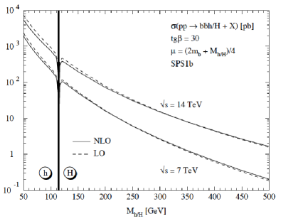
Figure 6: SUSY-QCD corrected production cross sections of light and heavy scalar MSSM Higgs bosons in association with $b\bar{b}$ pairs for the Snowmass point SPS1b [148]. See Ref. [144] for details.

The total cross section for scalar Higgs-boson radiation off bottom quarks at the LHC ($\sqrt{S}=14$ TeV) is shown in Fig. 6 for the MSSM benchmark scenario SPS1b [148] with $\tan\beta=30$. The four-flavor MSTW2008 pdfs [149] have been used. In Table 3 we show the individual contributions to the NLO cross section.

	$M_{A}$	$M_{H}$ [GeV]	$\delta^{H}_{\rm QCD}$	$\delta^{H}_{\rm SUSY}$	$\delta^{H}_{\rm SUSYrem}$
	100	113.9	0.27	$-0.38$	$0.3\times 10^{-4}$
	200	200	0.39	$-0.30$	$5.8\times 10^{-4}$
7 TeV​​	300	300	0.47	$-0.30$	$9.3\times 10^{-4}$
	400	400	0.53	$-0.30$	$1.5\times 10^{-3}$
	500	500	0.59	$-0.30$	$2.2\times 10^{-3}$
	100	113.9	0.17	$-0.38$	$0.5\times 10^{-4}$
	200	200	0.29	$-0.30$	$5.7\times 10^{-4}$
14 TeV​​	300	300	0.39	$-0.30$	$9.3\times 10^{-4}$
	400	400	0.45	$-0.30$	$1.5\times 10^{-3}$
	500	500	0.49	$-0.30$	$2.3\times 10^{-3}$

Table 3: Individual NLO corrections relative to the LO cross section for $pp\to b\bar{b}H+X$, as defined in Eq. (10), are shown for the LHC at two c.m. energies (7 TeV and 14 TeV) for the Snowmass point SPS1b [148].

The pure QCD corrections $\delta^{H}_{\rm QCD}$, the $\tan\beta$-enhanced SUSY-QCD corrections $\delta^{H}_{\rm SUSY}$, and the remainders of the SUSY-QCD corrections $\delta^{H}_{\rm SUSY-rem}$ are defined according to Eq. (12). The moderate NLO corrections in this MSSM scenario result from a compensation of the large, positive QCD corrections and large, negative SUSY-QCD corrections. The smallness of the SUSY-QCD remainder shows that the full NLO SUSY-QCD corrections are approximated extremely well by the $\tan\beta$-enhanced terms.

Let us briefly comment on heavy charged Higgs production at the LHC,

$$pp\,\rightarrow\,tH^{\pm}(b)+X.$$ (13)

In a two-Higgs doublet model of type II, like the minimal supersymmetric extension of the SM, the Yukawa coupling of the charged Higgs boson $H^{-}$ to a top quark and bottom antiquark is given by

$$g_{t\bar{b}H^{-}}=\sqrt{2}\left(\frac{m_{t}}{v}P_{R}\cot\beta+\frac{m_{b}}{v}P_{L}\tan\beta\right),$$ (14)

where $v=\sqrt{v_{u}^{2}+v_{d}^{2}}=(\sqrt{2}G_{F})^{-\frac{1}{2}}$ is the Higgs vacuum expectation value in the SM, with the Fermi constant $G_{F}=1.16637\times 10^{-5}\;\mbox{GeV}^{-2}$, and $P_{R/L}=(1\pm\gamma_{5})/2$ are the chirality projectors.

As in the case of neutral Higgs production with bottom quarks, the cross section for $pp\,\rightarrow\,tH^{\pm}(b)+X$ can be calculated in the four- or five-flavor schemes. Next-to-leading order predictions for heavy charged Higgs boson production at the LHC in a type-II two-Higgs-doublet model have been made in the past in both 5F [150, 151, 152, 153, 154, 155] and 4F schemes [156, 157], including also electroweak corrections [158, 159]. In Ref. [160], the NLO-QCD predictions have recently been updated and improved by adopting a dynamical scale setting procedure for the 5FS [161]. A thorough account of all sources of theoretical uncertainties has been given, and a Santander-matched prediction [142] for the four- and five-flavor scheme calculations has been provided. Reference [160] also includes results for a wide range of $\tan\beta$, which allows the comparison between theory and experiment for a large class of beyond-the-SM scenarios.

The cross section and uncertainty for the results of the 4F and 5F scheme calculations and their combination for $\sqrt{s}=14$ TeV are presented in Fig. 7. The dynamical choice of the factorisation scale in the five-flavor scheme calculation significantly improves the agreement between the four- and five-flavor schemes. The overall uncertainty of the matched cross-section prediction is approximately 20–30%, and includes the dependence on the renormalisation scale, the factorisation scale, the scale of the running bottom quark mass in the Yukawa coupling, as well as the input parameter uncertainties in the parton distribution functions, in the QCD coupling $\alpha_{s}$, and in the bottom quark mass.

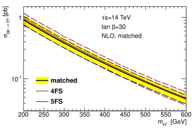
Figure 7: Santander-matched cross section and uncertainties for $pp\rightarrow tH^{\pm}+X$ at the LHC for 14 TeV. The 4F and 5F scheme results as well as the combined values are shown, together with their total uncertainties.

5.2 Higgs Bosons in the NMSSM

The NMSSM [123] extends the Higgs sector by an additional singlet superfield $\hat{S}$. This entails seven Higgs bosons after EWSB, which in the limit of the real NMSSM can be divided into three neutral purely CP-even, two neutral purely CP-odd and two charged Higgs bosons, and in total leads to five neutralinos. The NMSSM allows for the dynamical solution of the $\mu$ problem [162] through the scalar component of the singlet field acquiring a non-vanishing vacuum expectation value. Furthermore, the tree-level mass value of the lightest Higgs boson is increased by new contributions to the quartic coupling so that the radiative corrections necessary to shift the Higgs mass to $\sim 125$ GeV are less important than in the MSSM allowing for lighter stop masses and/or mixing and in turn less finetuning. The singlet admixture in the Higgs mass eigenstates entails reduced couplings to the SM particles. Together with the enlarged Higgs sector this leads to a plethora of interesting phenomenological scenarios and signatures. It is obvious that on the theoretical side the reliable interpretation of such BSM signatures and the disentanglement of different SUSY scenarios as well as their distinction from the SM situation require precise predictions of the SUSY parameters such as masses and Higgs couplings to other Higgs bosons including higher-order corrections. For the CP-conserving NMSSM the mass corrections are available at one-loop accuracy [163, 164, 165, 166, 167, 168, 169, 171, 172], and two loop results of O($\alpha_{t}\alpha_{s}+\alpha_{b}\alpha_{s}$) in the approximation of zero external momentum have been given in Ref. [169]. Recently, first corrections beyond order O($\alpha_{t}\alpha_{s}+\alpha_{b}\alpha_{s}$) have been given in [170]. In the complex case the one-loop corrections to the Higgs masses have been given in [173, 174, 175, 176, 177, 178] with the logarithmically enhanced two-loop effects presented in [179]. Quite recently we have provided the two-loop corrections to the Higgs boson masses of the CP-violating NMSSM in the Feynman diagrammatic approach with vanishing external momentum at O($\alpha_{t}\alpha_{s}$) [180]. Higher-order corrections to the trilinear Higgs self-coupling of the neutral NMSSM Higgs bosons have been provided in [181].

In the following the implications of the loop corrections in the real and complex NMSSM to the Higgs boson masses, and for the CP-conserving NMSSM, to the trilinear Higgs self-couplings shall be presented. To set up the notation the NMSSM Higgs sector is briefly discussed. The Higgs mass matrix is derived from the NMSSM Higgs potential, which is obtained from the superpotential, the soft SUSY breaking terms and from the $D$-term contributions. Denoting the Higgs doublet superfields, which couple to the up- and down-type quarks, by $\hat{H}_{u}$ and $\hat{H}_{d}$, respectively, and the singlet superfield by $\hat{S}$, the scale invariant NMSSM superpotential is given by

$$W_{\rm NMSSM}=W_{\rm MSSM}-\epsilon_{ij}\lambda\hat{S}\hat{H}^{i}_{d}\hat{H}^{j}_{u}+\frac{1}{3}\kappa\hat{S}^{3}\;,$$ (15)

with the $SU(2)_{L}$ indices $i,j=1,2$ and the totally antisymmetric tensor $\epsilon_{12}=1$. While the dimensionless parameters $\lambda$ and $\kappa$ can be complex in general, in case of CP-conservation they are taken to be real. In terms of the quark and lepton superfields and their charge conjugates, indicated by the superscript $c$, $\hat{Q},\hat{U}^{c},\hat{D}^{c},\hat{L},\hat{E}^{c}$, the MSSM superpotential $W_{\rm MSSM}$ reads

$$W_{\rm MSSM} = \epsilon_{ij}[y_{e}\hat{H}^{i}_{d}\hat{L}^{j}\hat{E}^{c}+y_{d}\hat{H}_{d}^{i}\hat{Q}^{j}\hat{D}^{c}$$ (16)

$$-y_{u}\hat{H}_{u}^{i}\hat{Q}^{j}\hat{U}^{c}]\;,$$

where the flavor and generation indices have been suppressed. In general the Yukawa couplings $y_{d},$ $y_{u}$ and $y_{e}$ in the MSSM superpotential Eq. (16) are complex. Neglecting generation mixing, their phases can be reabsorbed by redefining the quark fields. The MSSM $\mu$-term as well as the tadpole and bilinear terms of $\hat{S}$ are assumed to be zero. With the Higgs doublet and singlet component fields $H_{u}$, $H_{d}$ and $S$, the soft SUSY breaking NMSSM Lagrangian is given by

$$\mathcal{L}_{\rm soft} = {\cal L}_{\rm soft}^{\rm MSSM}-m_{S}^{2}|S|^{2}+(\epsilon_{ij}\lambda A_{\lambda}SH_{d}^{i}H_{u}^{j}$$ (17)

$$-\frac{1}{3}\kappa A_{\kappa}S^{3}+h.c.)\;,$$

where ${\cal L}_{\rm soft}^{\rm MSSM}$ denotes the soft SUSY breaking MSSM Lagrangian,

$${\cal L}_{\rm soft}^{\rm MSSM}\hskip 14.22636pt = -m_{H_{d}}^{2}H_{d}^{\dagger}H_{d}-m_{H_{u}}^{2}H_{u}^{\dagger}H_{u}-m_{Q}^{2}\tilde{Q}^{\dagger}\tilde{Q}$$ (18)

$$- m_{L}^{2}\tilde{L}^{\dagger}\tilde{L}-\,m_{U}^{2}\tilde{u}_{R}^{*}\tilde{u}_{R}-m_{D}^{2}\tilde{d}_{R}^{*}\tilde{d}_{R}$$

$$- m_{E}^{2}\tilde{e}_{R}^{*}\tilde{e}_{R}-\,(\epsilon_{ij}[y_{e}A_{e}H_{d}^{i}\tilde{L}^{j}\tilde{e}_{R}^{*}$$

$$+ y_{d}A_{d}H_{d}^{i}\tilde{Q}^{j}\tilde{d}_{R}^{*}-\,y_{u}A_{u}H_{u}^{i}\tilde{Q}^{j}\tilde{u}_{R}^{*}]+h.c.)$$

$$- \frac{1}{2}(M_{1}\tilde{B}\tilde{B}+M_{2}\,\tilde{W}_{k}\tilde{W}_{k}+M_{3}\tilde{G}\tilde{G}+h.c.)\;.$$

Here $\tilde{B}$, $\tilde{W}_{k}$ ($k=1,2,3$) and $\tilde{G}$ are the gaugino fields, and $\tilde{Q}=(\tilde{u}_{L},\tilde{d}_{L})^{T}$, $\tilde{L}=(\tilde{\nu}_{L},\tilde{e}_{L})^{T}$, where the tilde indicates the scalar components of the corresponding quark and lepton superfields. In the soft SUSY breaking NMSSM Lagrangian Eq. (17) the soft SUSY breaking mass parameters $m_{X}^{2}$ of the scalar fields $X=S,H_{d},H_{u},Q,U,D,L,E$ are real. The soft SUSY breaking trilinear couplings $A_{x}$ ($x=\lambda,\kappa,d,u,e$) and the gaugino mass parameters $M_{1},M_{2}$ and $M_{3}$, however, are complex in general but real in the CP-conserving case. Here, furthermore squark and slepton mixing between the generations is neglected and soft SUSY breaking terms linear and quadratic in the singlet field $S$ are set to zero. In the expansion of the Higgs boson fields about the VEVs two further phases, $\varphi_{u}$ and $\varphi_{s}$, appear,

$$H_{d} = \begin{pmatrix}\frac{1}{\sqrt{2}}(v_{d}+h_{d}+ia_{d})\\ h_{d}^{-}\end{pmatrix}~{},$$

$$H_{u} = e^{i\varphi_{u}}\begin{pmatrix}h_{u}^{+}\\ \frac{1}{\sqrt{2}}(v_{u}+h_{u}+ia_{u})\end{pmatrix}~{},$$

$$S = \frac{e^{i\varphi_{s}}}{\sqrt{2}}(v_{s}+h_{s}+ia_{s})~{},$$ (19)

describing the phase differences between the three VEVs $\langle H_{d}^{0}\rangle$, $\langle H_{u}^{0}\rangle$ and $\langle S\rangle$. For phase values $\varphi_{u}=\varphi_{s}=n\pi$, $n\in\mathbb{N}$, the fields $h_{i}$ and $a_{i}$ ($i=d,u,s$) are the pure CP-even and CP-odd parts of the neutral entries of $H_{u}$, $H_{d}$ and $S$. Exploiting the freedom in the phase choice of the Yukawa couplings to set $\varphi_{y_{u}}=-\varphi_{u}$ and assuming the down-type and charged lepton-type Yukawa couplings to be real, the quark and lepton mass terms yield real masses without any further phase transformation of the corresponding fields. Expansion about the VEVs leads to the Higgs boson mass matrix $M_{\phi\phi}$ that can be read off from the bilinear neutral Higgs field terms in the Higgs potential. CP-violation introduces a mixing between CP-even and CP-odd component fields, leading to a $6\times 6$ matrix in the basis $\phi=(h_{d},h_{u},h_{s},a_{d},a_{u},a_{s})^{T}$, which can be expressed in terms of three $3\times 3$ matrices $M_{hh},M_{aa}$ and $M_{ha}$,

$$M_{\phi\phi}=\begin{pmatrix}M_{hh}&M_{ha}\\ M_{ha}^{T}&M_{aa}\end{pmatrix}\;,$$ (20)

where $M_{hh}$ and $M_{aa}$ are symmetric matrices, describing the mixing among the CP-even components of the Higgs doublet and singlet fields and among the CP-odd components, respectively. In the CP-conserving case the matrix $M_{ha}$, which mixes CP-even and CP-odd components, vanishes. Due to the minimization conditions of the Higgs potential $V$ ($\phi=h_{d},h_{u},h_{s},a_{d},a_{u},a_{s}$),

$$t_{\phi}\equiv\left.\frac{\partial V}{\partial\phi}\right|_{\mbox{\scriptsize Min}}=0\;,$$ (21)

in the tree-level Higgs sector only one linearly independent phase combination $\varphi_{y}$ appears after applying the tadpole conditions for $\phi=a_{d}$ and $a_{s}$,

$$\varphi_{y}=\varphi_{\kappa}-\varphi_{\lambda}+2\varphi_{s}-\varphi_{u}\;.$$ (22)

The tadpole condition for $a_{u}$ does not lead to a new linearly independent condition. Hence the CP mixing due to $M_{ha}$ is governed by $\sin\varphi_{y}$ at tree-level. In the real case, the CP-odd tadpole conditions vanish and are thus automatically fulfilled.

In order to obtain the mass eigenstates first the $6\times 6$ rotation matrix ${\cal R}^{G}$ is applied to separate the would-be Goldstone boson field and then the matrix ${\cal R}$ to rotate to the mass eigenstates $H_{i}$ ($i=1,...,5$), yielding a diagonal mass matrix squared,

$$(H_{1},H_{2},H_{3},H_{4},H_{5},G)^{T} =$$ (23)

$${\cal R}^{D}(h_{d},h_{u},h_{s},a_{d},a_{u},a_{s})^{T}$$

$$\mbox{diag}((M_{H_{1}}^{(0)})^{2},...,(M_{H_{5}}^{(0)})^{2},0) = {\cal R}^{D}M_{\phi\phi}({\cal R}^{D})^{T}$$ (24)

with ${\cal R}^{D}\equiv{\cal R}{\cal R}^{G}$ and the superscript $(0)$ indicating tree-level masses. In the CP-conserving case the $6\times 6$ mass matrix $M_{\phi\phi}$ decomposes into $3\times 3$ Higgs mass matrices squared for the CP-even and CP-odd component Higgs fields, $M_{S}^{2}$ and $M_{A}^{2}$, respectively. The squared mass matrix $M_{S}^{2}$ is diagonalized through a rotation ${\cal R}^{S}$, yielding the CP-even mass eigenstates $H_{i}$ ($i=1,2,3$),

$$\begin{pmatrix}H_{1},H_{2},H_{3}\end{pmatrix}^{T}={\cal R}^{S}\begin{pmatrix}h_{d},h_{u},h_{s}\end{pmatrix}^{T},$$ (25)

$$\text{diag}((M_{H_{1}}^{(0)})^{2},(M_{H_{2}}^{(0)})^{2},(M_{H_{3}}^{(0)})^{2})={\cal R}^{S}{M_{S}^{2}}({\cal R}^{S})^{T}\;.$$ (26)

The mass eigenstates are ordered by ascending mass, $M_{H_{1}}^{(0)}\leq M_{H_{2}}^{(0)}\leq M_{H_{3}}^{(0)}$, where the superscript $(0)$ indicates the tree-level mass values. In the CP-odd Higgs sector a first rotation ${\cal R}^{G}$ is applied to separate the massless Goldstone boson $G$, followed by a rotation ${\cal R}^{P}$ to obtain the mass eigenstates $A_{i}\equiv A_{1},A_{2},G$ ($i=1,2,3$), cf. [172],

$$\begin{pmatrix}A_{1},A_{2},G\end{pmatrix}^{T}={\cal R}^{P}{\cal R}^{G}\begin{pmatrix}a_{d},a_{u},a_{s}\end{pmatrix}^{T},$$ (27)

$$\text{diag}((M_{A_{1}}^{(0)})^{2},(M_{A_{2}}^{(0)})^{2},0)={\cal R}^{P}{\cal R}^{G}{M_{A}^{2}}({\cal R}^{P}{\cal R}^{G})^{T}\;.$$ (28)

The parameters of the tree-level Higgs potential in the CP-violating NMSSM are

$$m_{H_{d}}^{2},m_{H_{u}}^{2},m_{S}^{2},g_{1},g_{2},v_{u},v_{d},v_{s},$$

$$\varphi_{s},\varphi_{u},\Re\lambda,\Im\lambda,\Re A_{\lambda},\Im A_{\lambda},\Re\kappa,\Im\kappa,\Re A_{\kappa},\Im A_{\kappa}~{}.$$ (29)

Some of the parameters are traded for more physical ones leading to the following parameter set

$$\underbrace{t_{h_{d}},t_{h_{u}},t_{h_{s}},t_{a_{d}},t_{a_{s}},M_{H^{\pm}}^{2},M_{W}^{2},M_{Z}^{2},e}_{\mbox{on-shell}},$$

$$\underbrace{\tan\beta,v_{s},\varphi_{s},\varphi_{u},\Re\lambda,\Im\lambda,\Re\kappa,\Im\kappa,\Re A_{\kappa}}_{\overline{\mbox{DR}}}\;.$$ (30)

In the renormalization performed for the computation of the one-loop corrected Higgs boson masses [178], the first part of parameters is defined via on-shell conditions. The tadpole parameters are chosen such that the linear terms or the Higgs fields in the Higgs potential also vanish at one-loop level. In a slight abuse of the language the tadpole renormalization conditions are therefore also called on-shell. The remaining parameters are interpreted as $\overline{\mbox{DR}}$ parameters. An alternative renormalization scheme uses the real part of $A_{\lambda}$ as a $\overline{\mbox{DR}}$ input parameter instead of the mass of the charged Higgs boson. In the computation of the one-loop masses in CP-conserving NMSSM two further renormalization schemes are applied, based on a pure on-shell, respectively, a pure $\overline{\mbox{DR}}$ scheme [172].

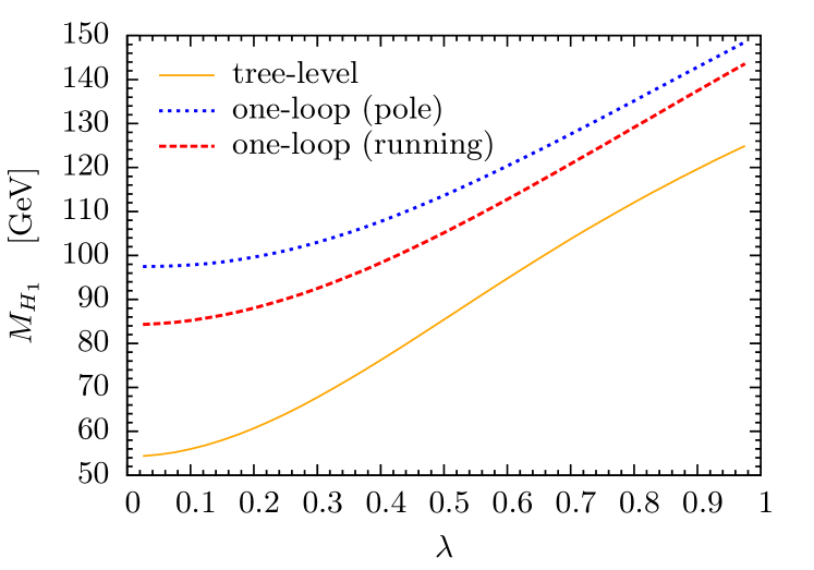
Figure 8: The mass $M_{H_{1}}$ of the lightest CP-even Higgs boson as function of $\lambda$; at tree-level (yellow/full), at one-loop level with the top quark pole mass (blue/dotted) and with the running $\overline{\mbox{DR}}$ top quark mass (red/dashed). From Ref. [172].

The loop corrections not only considerably alter the Higgs mass values but they also change the singlet admixtures in the various Higgs mass eigenstates and, in the case of CP-violation, their respective level of CP-violation, with significant phenomenological implications. For the results shown in the following, the scenarios have been chosen such that the constraints from LHC Higgs data and exclusion limits on the SUSY particles are fulfilled. The detailed parameter choices and applied constraints can be found in [172, 178]. Figure 8 shows for the CP-conserving case the mass of the lightest CP-even Higgs boson as function of $\lambda$, at tree-level and at one-loop level in the $\overline{\mbox{DR}}$ scheme with the top quark mass taken as the running $\overline{\mbox{DR}}$ mass $m_{t}=150.6$ GeV at the scale $Q_{0}=300$ GeV in one case and as the pole mass $M_{t}=173.3$ GeV in the other case. The tree-level mass increases with rising $\lambda$ due to the NMSSM contribution $\sim\lambda^{2}\sin^{2}2\beta$ from the Higgs quartic coupling. The one-loop corrections are important, increasing the $H_{1}$ mass by up to $\sim 44$ GeV, and strongly depend on the value of the top quark mass, which reflects the fact that the main part of the higher-order corrections stem from the top sector. An estimate of the missing higher-order corrections can be obtained by investigating the influence of the renormalization scale $Q_{0}$. The residual theoretical uncertainties due to missing higher-order corrections can thus be estimated to O(10%). These uncertainties as well as the dependence of the corrections on the value of top quark mass and/or the choice of the renormalization scheme, of course, get reduced once two-loop corrections are taken into account.

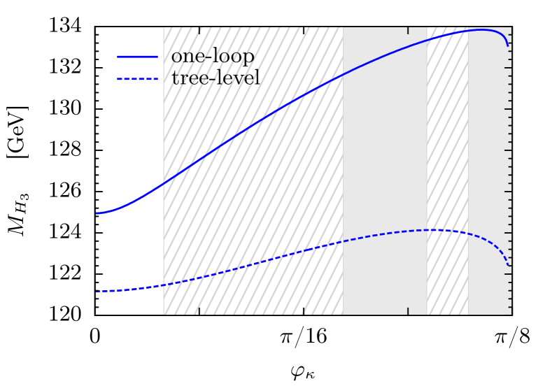
Figure 9: Tree-level (dashed) and one-loop (full) mass $M_{H_{3}}$ as a function of $\varphi_{\kappa}$. The exclusion region due to LEP, Tevatron and LHC data is shown as grey area, the region with the SM-like Higgs boson not being compatible with an excess of data around 125 GeV as dashed area. Taken from Ref. [178].

In the NMSSM CP-violation in the Higgs sector can already occur at tree-level due to a non-vanishing phase $\varphi_{y}$. The effect of a non-vanishing phase $\varphi_{\kappa}$ is demonstrated in Fig. 9 which shows the tree-level and one-loop mass of $H_{3}$ which in the chosen scenario corresponds to a SM-like Higgs boson with mass around 125 GeV. As expected, the mass exhibits already at tree-level a sensitivity to the CP-violating phase $\varphi_{\kappa}$. This dependence is even more pronounced at one-loop level, changing the $H_{3}$ mass value by up to 9 GeV for $\varphi_{\kappa}\in[0,\pi/8]$. The grey areas are the parameter regions which are excluded due to the experimental constraints from LEP, Tevatron and LHC, the dashed region excludes the parameter regions where the criteria of compatibility with the Higgs excess around 125 GeV cannot be fulfilled any more. See [178] for details. The two-loop corrections at O($\alpha_{t}\alpha_{s}$) based on a mixed $\overline{\mbox{DR}}$-on-shell renormalization scheme [180] have been provided for both $\overline{\mbox{DR}}$ and on-shell renormalization in the top/stop sector. For the light Higgs boson masses, the corrections turn out to be important and are of the order of 5-10% for the SM-like Higgs boson, depending on the adopted top/stop renormalization scheme. An estimate of the remaining theoretical uncertainties due to missing higher order corrections, by varying the renormalization scheme in the top/stop sector, shows, that the uncertainty is reduced from one- to two-loop order. The difference in the mass values of the SM-like Higgs boson for the two schemes decreases from 15-25% to below 1.5%. These two-loop corrections together with the one-loop corrections have been implemented in the Fortran package Nmssmcalc [182], which provides besides the loop-corrected Higgs boson masses in the real and complex NMSSM also the NMSSM Higgs branching ratios including the state-of-the-art higher order corrections and the relevant off-shell decays.

Not only the Higgs boson masses but also the Higgs self-interactions arise from the Higgs potential, and they can hence not be separated from each other. In order to consistently describe the Higgs sector including higher-order corrections, it is therefore not sufficient to only correct the Higgs boson masses. The trilinear and quartic Higgs self-interactions have to be evaluated at the same order in perturbation theory and within the same renormalization scheme as the Higgs boson masses to allow for a consistent description of the Higgs boson phenomenology. The trilinear Higgs self-couplings play a role in the determination of the Higgs boson branching ratios into SM particles, in the evaluation of Higgs-to-Higgs decays and in Higgs pair production processes. The one-loop corrections to the trilinear Higgs self-couplings of the CP-conserving NMSSM in the Feynman-diagrammatic approach have been evaluated in [181] by applying the mixed $\overline{\mbox{DR}}$-on-shell renormalization scheme, used also for the one-loop corrections to the Higgs boson masses presented here and introduced in [172]. Table 4 summarizes the Higgs pair production cross section values for gluon fusion in scenarios where the heavy CP-even $H_{3}$ is large enough to allow for the production of a pair of SM-like Higgs bosons. Here $\sigma_{T}$ denotes the cross sections calculated using the effective tree-level trilinear Higgs couplings, while the cross section values $\sigma_{L}$ use the effective loop-corrected trilinear Higgs self-couplings. The differences in the cross sections due to the inclusion of loop corrections in the trilinear Higgs self-couplings can be substantial, ranging from nearly 40% to almost 90% in terms of the tree-level cross section for the chosen scenarios.

	$\sigma_{\text{T}}[fb]$	$\sigma_{\text{L}}[fb]$	$\delta$
Point 1	432.4(3)	96.08(7)	-0.78
Point 2	181.5(3)	55.92(2)	-0.69
Point 3	533.9(4)	265.5(2)	-0.50
Point 4	413.3(3)	53.05(4)	-0.87
Point 5	43.24(2)	69.05(5)	0.60

Table 4: The total cross sections in fb for $pp\to H_{i}H_{i}$ through gluon fusion at $\sqrt{s}=14$ TeV, with $H_{i}$ being the SM-like Higgs boson, evaluated with tree-level ($\sigma_{T}$) and loop-corrected ($\sigma_{L}$) effective trilinear Higgs couplings. The deviation in the cross sections is quantified by $\delta=(\sigma_{L}-\sigma_{T})/\sigma_{T}$. For details, see [181].

The NMSSM with its increased parameter set in the Higgs sector and in the soft SUSY breaking Lagrangian allows for a large playground in Higgs boson phenomenology. We have performed extensive parameter scans in the NMSSM by taking into account the constraints from the LHC Higgs data, from the LHC searches for SUSY particles and the ones arising from Dark Matter, low-energy observables and from the LEP and Tevatron data. In Ref. [183] we have shown that scenarios can be found that are compatible with all constraints and can accommodate the enhanced di-photon final state rate, which was then still present both in the ATLAS and CMS data. This can be achieved even for rather light stop masses without large fine-tuning. The scan of Ref. [184] shows that there is a substantial amount of parameter space with Higgs boson masses and couplings compatible with the LHC results. If guided by fine-tuning considerations, the next-to-lightest Higgs boson $H_{2}$ being the SM-like state is favoured. However, dropping this assumption also leads to $H_{1}$ being the SM-like scalar or even scenarios where $H_{1}$ and $H_{2}$ are almost degenerate in mass and close to 125 GeV. The extensive survey of the NMSSM performed in [185] revealed that the natural NMSSM, which we defined to be characterized by rather small $\kappa$ values, low $\tan\beta$ and an overall Higgs spectrum below about 530 GeV, can be tested at the next run of the LHC with a c.m. energy of 13 TeV. This relies on exploiting also Higgs production from Higgs-to-Higgs decays and Higgs decays into a Higgs and gauge boson pair. Focusing subsequently on these cascade decays, we found that within the NMSSM exotic final state signatures with multi-photon and/or multi-fermion final states at significant rates can be possible arising from one or several Higgs cascade decays. They furthermore give access to the trilinear Higgs self-couplings. These interesting and sometimes unique signatures should be taken into account when designing analysis strategies for the LHC.

6 Higgs Coupling Measurements and Implications for New Physics Scales

According to the present data the observed Higgs particle is in good agreement with SM expectations. The experimental uncertainties are still large though and allow for interpretations in models beyond the SM as we have seen in the previous sections. The high-energy and high-luminosity run of the LHC will increase the precision on the data. Thus the precision on the Higgs couplings will improve from at present several tens of percent to about 10% in the high-luminosity (HL-LHC) option [186, 187, 188, 189, 190]. A future $e^{+}e^{-}$ linear collider (LC) [189, 190, 191, 192, 193, 194] can improve the accuracy to about 1%, cf. Table 5. Deviations in the interactions of the Higgs boson from their SM values can arise if the Higgs mixes with other scalars, if it is a composite particle or a mixture between an elementary and composite state (partial compositeness) or through loop contributions from other new particles. Depending on the strength and type of the coupling between the new physics and the Higgs boson, the limits derived from the Higgs measurements can exceed those from direct searches, EW precision measurements or flavor physics. Higgs precision analyses can thus be sensitive to new physics residing at scales much higher than the VEV and open a unique window to new physics sectors that are not yet strongly constrained by existing results. The effective field theory approach allows to study a large class of BSM models in terms of a well defined quantum field theory. It cannot account, however, for effects that arise from light particles or from Higgs decays into new non-SM particles. In order to give a complete picture of BSM effects in the Higgs sectors, therefore also specific BSM models capturing such features have to be studied. In the following a few examples for both approaches shall be highlighted, based on Ref. [195], where more details and further investigated models can be found.

coupl.	LHC	HL-LHC	LC	HL-LC	comb.
$hWW$	0.09	0.08	0.011	0.006	0.005
$hZZ$	0.11	0.08	0.008	0.005	0.004
$htt$	0.15	0.12	0.040	0.017	0.015
$hbb$	0.20	0.16	0.023	0.012	0.011
$h\tau\tau$	0.11	0.09	0.033	0.017	0.015
$h\gamma\gamma$	0.20	0.15	0.083	0.035	0.024
$hgg$	0.30	0.08	0.054	0.028	0.024
$h_{\scriptsize\mathrm{invis}}$	—	—	0.008	0.004	0.004

Table 5: Expected accuracy at the 68% C.L. with which fundamental and derived Higgs couplings can be measured; the deviations are defined as $g=g_{\scriptsize\mbox{SM}}[1\pm\Delta]$ compared to the Standard Model at the LHC/HL-LHC (luminosities 300 and 3000 fb^-1), LC/HL-LC (energies 250+500 GeV / 250+500 GeV+1 TeV and luminosities 250+500 fb^-1 / 1150+1600+2500 fb^-1), and in combined analyses of HL-LHC and HL-LC. For invisible Higgs decays the upper limit on the underlying couplings is given. Taken from [195].

Based on operator expansions [3, 4, 5, 6] deviations from the SM coupling values can be estimated to be of the order of

$$g=g_{\scriptsize\mbox{SM}}[1+\Delta]\;:\;\Delta={\cal O}(v^{2}/\Lambda^{2})\;,$$ (31)

where $v$ denotes the VEV of the SM field and $\Lambda\gg v$ the characteristic BSM scale. Note that this does not hold in case the underlying model violates the decoupling theorem. Assuming experimental accuracies of $\Delta=0.2$ down to $0.01$ implies a sensitivity to scales of order $\Lambda\sim 550$ GeV up to 2.5 TeV. The smaller bound is complementary to direct LHC searches whereas the larger of the two bounds in general exceeds the direct LHC search range. If the Higgs coupling deviations are due to vertex corrections generated by virtual contributions of new particles, a suppression factor of $1/(16\pi^{2})$ has to be taken into account in addition to potentially small couplings between the SM and the new fields. Hence only new scales not in excess of about $M<v/(4\pi\sqrt{\Delta})\sim 200$ GeV can be probed, which in most models is much less than the direct search reach at the LHC.

The extracted limits on the effective scales $\Lambda_{*}$ from the contributions of the dimension-6 operators taking into account the coupling precisions of Table 5 are shown in Fig. 10. They have been obtained with Sfitter [186, 187, 188] after defining the effective scales $\Lambda_{*}$ that are obtained by factoring out from the operators typical coefficients like couplings and loop factors. Furthermore, in the loop-induced couplings to the gluons and photons only the contributions from the contact terms are kept. The effects of the loop terms are already disentangled at the level of the input values $\Delta$.

Figure 10: Effective NP scales $\Lambda_{\ast}$ extracted from the Higgs coupling measurements collected in Table 5. (The ordering of the columns from left to right corresponds to the legend from up to down.) For details, see [195].

type-I type-II lepton-specific flipped

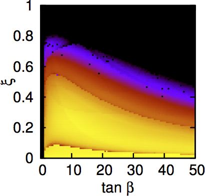
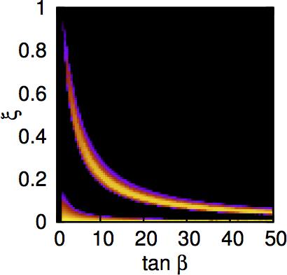
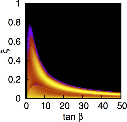
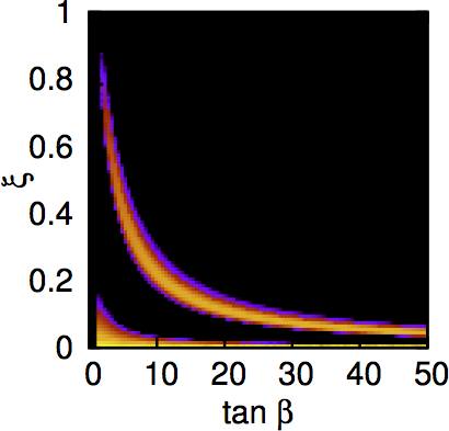
Figure 11: Allowed ranges for the modification parameter $\xi$ in a 2HDM in the decoupling limit, based on data from Ref. [202]. The plots show the correlated relative log-likelihood $-2\,\Delta(\log\cal L)$ as a function of $\tan\beta$, from Ref. [203].

As a last example, the interpretation of the current Higgs coupling measurements in terms of a 2-Higgs-Doublet Model (2HDM) is shown. Here the Higgs coupling modifications are due to mixing effects, with the physical states being mixtures of the components of two doublets $\phi_{1}$ and $\phi_{2}$ [196, 197, 198, 199, 200]. The scalar potential can be cast into the form

$$V = m_{11}|\phi_{1}|^{2}+m_{22}^{2}|\phi_{2}|^{2}-m_{12}^{2}(\phi_{1}^{\dagger}\phi_{2}+\text{h.c})$$ (32)

$$+ \lambda_{1}|\phi_{1}|^{4}+\lambda_{2}|\phi_{2}|^{4}+\lambda_{3}|\phi_{1}|^{2}|\phi_{2}|^{2}+\lambda_{4}|\phi_{1}^{\dagger}\phi_{2}|^{2}$$

$$+ \frac{1}{2}\lambda_{5}[(\phi_{1}^{\dagger}\phi_{2})^{2}+\text{h.c}]\,.$$

By imposing a global $\mathbb{Z}_{2}$ discrete symmetry, under which $\phi_{1,2}\to\mp\phi_{1,2}$, it can be achieved that one type of fermions couples only to one Higgs doublet. This ensures the natural suppression of flavor-changing neutral currents. In the potential Eq. (32) such a symmetry has been assumed, softly broken by the term $\propto m_{12}^{2}$. The Higgs fields acquire vacuum expectations values, $v_{1}$ and $v_{2}$, with $v^{2}_{1}+v^{2}_{2}=v^{2}$ and $\tan\beta=v_{2}/v_{1}$. Depending on the $\mathbb{Z}_{2}$ charge assignments, the following four cases of coupling the Higgs doublets to fermions are possible [201]:

• type I: all fermions couple only to $\phi_{2}$;

• type II: up-/down-type fermions couple to $\phi_{2}$/$\phi_{1}$, respectively;

• lepton-specific: quarks couple to $\phi_{2}$ and charged leptons couple to $\phi_{1}$;

• flipped: up-type quarks and leptons couple to $\phi_{2}$ and down-type quarks couple to $\phi_{1}$.

Note that the MSSM is a special case of the general 2HDM type-II. After EWSB the Higgs sector features five physical Higgs states, two neutral CP-even ones $h^{0},H^{0}$, one neutral CP-odd one $A^{0}$ and two charged Higgs bosons $H^{\pm}$. In the so-called decoupling limit the masses of the heavy Higgs bosons $H^{0},A^{0}$ and $H^{\pm}$ are much larger than $v$ and the physics of the light Higgs boson $h^{0}$ can be described by an effective theory [200]. The properties of the lightest CP-even Higgs boson $h^{0}$ are close to the SM. Figure 11 shows the shape of the decoupling limit in the different model setups. Type-I models are preferred in a comparably wide parameter range which is due to the fact that it separates Higgs couplings to gauge bosons and fermions. This makes it easy to accommodate the slightly enhanced $H\to\tau\tau$ rate. So far none of the analyses based on the Higgs couplings measured at the LHC has shown a clear sign for such mixing effects. Further discussions within typical scenarios and models that are archetypal examples for a much larger class of models can be found in [195].

7 Conclusions

While the properties of the new particle recently discovered at the LHC are consistent with those expected for the Higgs boson of the Standard Model, the present experimental precision still leaves room for interpretations within BSM extensions. These can be either strongly interacting theories, or rely on weak interactions as e.g. supersymmetric models. In order to test a wide range of new physics scenarios in a more model-independent way, the effective Lagrangian approach can be applied for the interpretation of the data. Such an approach is valid as long as the new physics scale is well above the Higgs mass value. The interpretation of LHC data through effective Lagrangians must be complemented by analyses within specific models in order to take into account effects from low-lying resonances.

Composite Higgs models are specific realizations of models based on strong dynamics. They are heavily constrained by electroweak precision data, however still in accordance with the LHC data, in particular when new heavy quarks are taken into account. We have discussed in detail the compatibility of composite Higgs models with the LHC results and the role of new heavy quarks in the loop-induced single and double Higgs production processes through gluon fusion.

Supersymmetric models, on the other hand, are weakly interacting. In the minimal version, the MSSM, a sufficiently large Higgs mass of 125 GeV can only be achieved for heavy stops and/or large mixing, whereas the next-to-minimal model (NMSSM) with its enlarged parameter space can accommodate the Higgs mass more easily. In order to distinguish various SUSY models from each other, and from other BSM extensions, higher-order corrections are essential. Only the high-precision calculations allow to correctly interpret the experimental data. We have reported on recent progress in higher-order calculations to MSSM Higgs boson production in association with heavy quarks and on the calculation of NMSSM Higgs boson masses and self-interactions.

Finally, we have presented the conclusions that can be drawn on the scale of new physics from high-precision measurements of the Higgs couplings at the upcoming LHC runs, and at a future $e^{+}e^{-}$ linear collider.

References

- [1] G. Aad et al. [ATLAS Collaboration], Phys. Lett. B 716 (2012) 1 [arXiv:1207.7214 [hep-ex]]; G. Aad et al. [ATLAS Collaboration], ATLAS-CONF-2012-162.
- [2] S. Chatrchyan et al. [CMS Collaboration], Phys. Lett. B 716 (2012) 30 [arXiv:1207.7235 [hep-ex]]; S. Chatrchyan et al. [CMS Collaboration], CMS-PAS-HIG-12-045.
- [3] C. J. C. Burges and H. J. Schnitzer, Nucl. Phys. B 228 (1983) 464.
- [4] C. N. Leung, S. T. Love and S. Rao, Z. Phys. C 31 (1986) 433.
- [5] W. Buchmuller and D. Wyler, Nucl. Phys. B 268 (1986) 621.
- [6] B. Grzadkowski, M. Iskrzynski, M. Misiak and J. Rosiek, JHEP 1010 (2010) 085 [arXiv:1008.4884 [hep-ph]].
- [7] G. F. Giudice, C. Grojean, A. Pomarol and R. Rattazzi, JHEP 0706 (2007) 045 [hep-ph/0703164].
- [8] B. Grinstein and M. Trott, Phys. Rev. D 76 (2007) 073002 [arXiv:0704.1505 [hep-ph]].
- [9] R. Contino, M. Ghezzi, C. Grojean, M. Muhlleitner and M. Spira, JHEP 1307 (2013) 035 [arXiv:1303.3876 [hep-ph]].
- [10] R. Contino, M. Ghezzi, C. Grojean, M. Muhlleitner and M. Spira, Comput. Phys. Commun. 185 (2014) 3412 [arXiv:1403.3381 [hep-ph]].
- [11] J. Elias-Miro, J. R. Espinosa, E. Masso, A. Pomarol, JHEP 1311 (2013) 066 [arXiv:1308.1879 [hep-ph]].
- [12] G. Isidori and M. Trott, JHEP 1402 (2014) 082 [arXiv:1307.4051 [hep-ph], arXiv:1307.4051].
- [13] I. Brivio, T. Corbett, O. J. P. Eboli, M. B. Gavela, J. Gonzalez-Fraile, M. C. Gonzalez-Garcia, L. Merlo and S. Rigolin, JHEP 1403 (2014) 024 [arXiv:1311.1823 [hep-ph]].
- [14] A. Pomarol and F. Riva, JHEP 1401 (2014) 151 [arXiv:1308.2803 [hep-ph]].
- [15] R. S. Gupta, A. Pomarol and F. Riva, arXiv:1405.0181 [hep-ph].
- [16] K. Agashe, R. Contino and A. Pomarol, Nucl. Phys. B 719 (2005) 165 [hep-ph/0412089].
- [17] R. Contino, L. Da Rold and A. Pomarol, Phys. Rev. D 75 (2007) 055014 [hep-ph/0612048].
- [18] A. Djouadi, J. Kalinowski and M. Spira, Comput. Phys. Commun. 108 (1998) 56 [hep-ph/9704448].
- [19] A. Djouadi, M. M. Muhlleitner and M. Spira, Acta Phys. Polon. B 38 (2007) 635 [hep-ph/0609292].
- [20] A. David et al. [LHC Higgs Cross Section Working Group Collaboration], arXiv:1209.0040 [hep-ph].
- [21] A. Biekoetter, A. Knochel, M. Krämer, D. Liu and F. Riva, arXiv:1406.7320 [hep-ph].
- [22] J. R. Espinosa, C. Grojean, M. Muhlleitner and M. Trott, JHEP 1205 (2012) 097 [arXiv:1202.3697 [hep-ph]].
- [23] J. R. Espinosa, C. Grojean, M. Muhlleitner and M. Trott, JHEP 1212 (2012) 045 [arXiv:1207.1717 [hep-ph]].
- [24] J. R. Espinosa, M. Muhlleitner, C. Grojean and M. Trott, JHEP 1209 (2012) 126 [arXiv:1205.6790 [hep-ph]].
- [25] A. Djouadi, W. Kilian, M. Muhlleitner and P. M. Zerwas, Eur. Phys. J. C 10 (1999) 27 [hep-ph/9903229].
- [26] A. Djouadi, W. Kilian, M. Muhlleitner and P. M. Zerwas, Eur. Phys. J. C 10 (1999) 45 [hep-ph/9904287].
- [27] O. J. P. Eboli, G. C. Marques, S. F. Novaes and A. A. Natale, Phys. Lett. B 197 (1987) 269.
- [28] E. W. N. Glover and J. J. van der Bij, Nucl. Phys. B 309 (1988) 282.
- [29] D. A. Dicus and C. Kao, Phys. Rev. D 38 (1988) 1008 [Erratum-ibid. D 42 (1990) 2412].
- [30] T. Plehn, M. Spira and P. M. Zerwas, Nucl. Phys. B 479 (1996) 46 [Erratum-ibid. B 531 (1998) 655] [hep-ph/9603205].
- [31] W. Y. Keung, Mod. Phys. Lett. A 2 (1987) 765.
- [32] D. A. Dicus, K. J. Kallianpur and S. S. D. Willenbrock, Phys. Lett. B 200 (1988) 187.
- [33] A. Dobrovolskaya and V. Novikov, Z. Phys. C 52 (1991) 427.
- [34] A. Abbasabadi, W. W. Repko, D. A. Dicus and R. Vega, Phys. Rev. D 38 (1988) 2770.
- [35] V. D. Barger, T. Han and R. J. N. Phillips, Phys. Rev. D 38 (1988) 2766.
- [36] M. Moretti, S. Moretti, F. Piccinini, R. Pittau and A. D. Polosa, JHEP 0502 (2005) 024 [hep-ph/0410334].
- [37] J. R. Ellis, M. K. Gaillard and D. V. Nanopoulos, Nucl. Phys. B106 (1976) 292.
- [38] M. A. Shifman, A. I. Vainshtein, M. B. Voloshin and V. I. Zakharov, Sov. J. Nucl. Phys. 30 (1979) 711 [Yad. Fiz. 30 (1979) 1368].
- [39] B. A. Kniehl and M. Spira, Z. Phys. C69 (1995) 77.
- [40] J. Baglio, A. Djouadi, R. Grober, M. M. Muhlleitner, J. Quevillon and M. Spira, JHEP 1304 (2013) 151 [arXiv:1212.5581 [hep-ph]].
- [41] J. Grigo, J. Hoff, K. Melnikov and M. Steinhauser, Nucl. Phys. B 875 (2013) 1 [arXiv:1305.7340 [hep-ph]].
- [42] J. Grigo, J. Hoff, K. Melnikov and M. Steinhauser, PoS RADCOR 2013 (2013) 006 [arXiv:1311.7425 [hep-ph]].
- [43] F. Maltoni, E. Vryonidou and M. Zaro, arXiv:1408.6542 [hep-ph].
- [44] D. de Florian and J. Mazzitelli, Phys. Lett. B 724 (2013) 306 [arXiv:1305.5206 [hep-ph]].
- [45] D. de Florian and J. Mazzitelli, Phys. Rev. Lett. 111 (2013) 201801 [arXiv:1309.6594 [hep-ph]].
- [46] J. Grigo, K. Melnikov and M. Steinhauser, arXiv:1408.2422 [hep-ph].
- [47] T. Figy, C. Oleari and D. Zeppenfeld, Phys. Rev. D 68 (2003) 073005 [hep-ph/0306109].
- [48] G. Altarelli, R. K. Ellis and G. Martinelli, Nucl. Phys. B 157 (1979) 461.
- [49] T. Han and S. Willenbrock, Phys. Lett. B 273 (1991) 167.
- [50] J. Kubar-Andre and F. E. Paige, Phys. Rev. D 19 (1979) 221.
- [51] O. Brein, A. Djouadi and R. Harlander, Phys. Lett. B 579 (2004) 149 [hep-ph/0307206].
- [52] B. A. Kniehl, Phys. Rev. D 42 (1990) 2253.
- [53] D. B. Kaplan and H. Georgi, Phys. Lett. B 136 (1984) 183.
- [54] S. Dimopoulos and J. Preskill, Nucl. Phys. B 199 (1982) 206.
- [55] T. Banks, Nucl. Phys. B 243 (1984) 125.
- [56] D. B. Kaplan, H. Georgi and S. Dimopoulos, Phys. Lett. B 136 (1984) 187.
- [57] H. Georgi, D. B. Kaplan and P. Galison, Phys. Lett. B 143 (1984) 152.
- [58] H. Georgi and D. B. Kaplan, Phys. Lett. B 145 (1984) 216.
- [59] M. J. Dugan, H. Georgi and D. B. Kaplan, Nucl. Phys. B 254 (1985) 299.
- [60] D. B. Kaplan, Nucl. Phys. B 365 (1991) 259.
- [61] R. Contino, T. Kramer, M. Son and R. Sundrum, JHEP 0705 (2007) 074 [hep-ph/0612180].
- [62] O. Matsedonskyi, G. Panico and A. Wulzer, JHEP 1301 (2013) 164 [arXiv:1204.6333 [hep-ph]].
- [63] M. Redi and A. Tesi, JHEP 1210 (2012) 166 [arXiv:1205.0232 [hep-ph]].
- [64] G. Panico, M. Redi, A. Tesi and A. Wulzer, JHEP 1303 (2013) 051 [arXiv:1210.7114 [hep-ph]].
- [65] D. Pappadopulo, A. Thamm and R. Torre, JHEP 1307 (2013) 058 [arXiv:1303.3062 [hep-ph]].
- [66] D. Marzocca, M. Serone and J. Shu, JHEP 1208 (2012) 013 [arXiv:1205.0770 [hep-ph]].
- [67] A. Pomarol and F. Riva, JHEP 1208 (2012) 135 [arXiv:1205.6434 [hep-ph]].
- [68] J. R. Espinosa, C. Grojean and M. Muhlleitner, JHEP 1005 (2010) 065 [arXiv:1003.3251 [hep-ph]].
- [69] R. Contino, C. Grojean, M. Moretti, F. Piccinini and R. Rattazzi, JHEP 1005 (2010) 089 [arXiv:1002.1011 [hep-ph]].
- [70] R. Grober and M. Muhlleitner, JHEP 1106 (2011) 020 [arXiv:1012.1562 [hep-ph]].
- [71] R. Contino, C. Grojean, D. Pappadopulo, R. Rattazzi and A. Thamm, JHEP 1402 (2014) 006 [arXiv:1309.7038 [hep-ph]].
- [72] K. Agashe and R. Contino, Nucl. Phys. B 742 (2006) 59 [hep-ph/0510164].
- [73] R. Barbieri, B. Bellazzini, V. S. Rychkov and A. Varagnolo, Phys. Rev. D 76 (2007) 115008 [arXiv:0706.0432 [hep-ph]].
- [74] A. Pomarol and J. Serra, Phys. Rev. D 78 (2008) 074026 [arXiv:0806.3247 [hep-ph]].
- [75] R. Contino, arXiv:1005.4269 [hep-ph].
- [76] M. E. Peskin and T. Takeuchi, Phys. Rev. D 46 (1992) 381.
- [77] L. Lavoura and J. P. Silva, Phys. Rev. D 47 (1993) 2046.
- [78] P. Lodone, JHEP 0812 (2008) 029 [arXiv:0806.1472 [hep-ph]].
- [79] M. Gillioz, Phys. Rev. D 80 (2009) 055003 [arXiv:0806.3450 [hep-ph]].
- [80] C. Anastasiou, E. Furlan and J. Santiago, Phys. Rev. D 79 (2009) 075003 [arXiv:0901.2117 [hep-ph]].
- [81] C. Grojean, O. Matsedonskyi and G. Panico, JHEP 1310 (2013) 160 [arXiv:1306.4655 [hep-ph]].
- [82] M. Gillioz, R. Grober, A. Kapuvari and M. Muhlleitner, JHEP 1403 (2014) 037 [arXiv:1311.4453 [hep-ph]].
- [83] M. Gillioz, R. Grober, C. Grojean, M. Muhlleitner and E. Salvioni, JHEP 1210 (2012) 004 [arXiv:1206.7120 [hep-ph]].
- [84] A. Falkowski, Phys. Rev. D 77 (2008) 055018 [arXiv:0711.0828 [hep-ph]].
- [85] I. Low and A. Vichi, Phys. Rev. D 84 (2011) 045019 [arXiv:1010.2753 [hep-ph]].
- [86] A. Azatov and J. Galloway, Phys. Rev. D 85 (2012) 055013 [arXiv:1110.5646 [hep-ph]].
- [87] E. Furlan, JHEP 1110 (2011) 115 [arXiv:1106.4024 [hep-ph]].
- [88] U. Baur, T. Plehn and D. L. Rainwater, Phys. Rev. Lett. 89 (2002) 151801 [hep-ph/0206024].
- [89] T. E. W. Group [CDF and D0 Collaborations], arXiv:0908.2171 [hep-ex].
- [90] M. Redi and A. Weiler, JHEP 1111 (2011) 108 [arXiv:1106.6357 [hep-ph]].
- [91] C. Delaunay, C. Grojean and G. Perez, JHEP 1309 (2013) 090 [arXiv:1303.5701 [hep-ph]].
- [92] G. Aad et al. [ATLAS Collaboration], JHEP 1301 (2013) 029 [arXiv:1210.1718 [hep-ex]].
- [93] S. Chatrchyan et al. [CMS Collaboration], Phys. Rev. D 87 (2013) 5, 052017 [arXiv:1301.5023 [hep-ex]].
- [94] L. Da Rold, C. Delaunay, C. Grojean and G. Perez, JHEP 1302 (2013) 149 [arXiv:1208.1499 [hep-ph]].
- [95] M. Redi, Eur. Phys. J. C 72 (2012) 2030 [arXiv:1203.4220 [hep-ph]].
- [96] N. Vignaroli, Phys. Rev. D 86 (2012) 115011 [arXiv:1204.0478 [hep-ph]].
- [97] CMS Collaboration, CMS-PAS-EXO-11-099; arXiv:1203.5410 [hep-ex]; CMS-PAS-EXO-11-036; JHEP 1205 (2012) 123 [arXiv:1204.1088 [hep-ex]]; Phys. Rev. Lett. 107 (2011) 271802 [arXiv:1109.4985 [hep-ex]].
- [98] ATLAS Collaboration, arXiv:1202.3076 [hep-ex]; arXiv:1202.3389 [hep-ex]; arXiv:1202.6540 [hep-ex]; arXiv:1202.5520 [hep-ex].
- [99] CDF Collaboration, Phys. Rev. Lett. 107 (2011) 261801 [arXiv:1107.3875 [hep-ex]]; Phys. Rev. Lett. 106 (2011) 141803 [arXiv:1101.5728 [hep-ex]].
- [100] M. Aliev, H. Lacker, U. Langenfeld, S. Moch, P. Uwer and M. Wiedermann, Comput. Phys. Commun. 182 (2011) 1034 [arXiv:1007.1327 [hep-ph]].
- [101] S. Chatrchyan et al. [CMS Collaboration], JHEP 1212 (2012) 035 [arXiv:1209.4533 [hep-ex]].
- [102] The ATLAS Collaboration, ATLAS-CONF-2013-018, ATLAS-CONF-2013-051, ATLAS-CONF-2013-056, and ATLAS-CONF-2013-060.
- [103] The CMS Collaboration, CMS PAS B2G-12-019.
- [104] S. Chatrchyan et al. [CMS Collaboration], arXiv:1311.7667 [hep-ex].
- [105] The CMS Collaboration, CMS-PAS-HIG-13-005.
- [106] The ATLAS Collaboration, ATLAS-CONF-2013-034.
- [107] D. V. Volkov and V. P. Akulov, Phys. Lett. B 46 (1973) 109.
- [108] J. Wess and B. Zumino, Nucl. Phys. B 70 (1974) 39.
- [109] P. Fayet, Phys. Lett. B 64 (1976) 159.
- [110] P. Fayet and S. Ferrara, Phys. Rept. 32 (1977) 249.
- [111] P. Fayet, Phys. Lett. B 69 (1977) 489.
- [112] P. Fayet, Phys. Lett. B 84 (1979) 416.
- [113] G. R. Farrar and P. Fayet, Phys. Lett. B 76 (1978) 575.
- [114] E. Witten, Nucl. Phys. B 188 (1981) 513.
- [115] H. P. Nilles, Phys. Rept. 110 (1984) 1.
- [116] H. E. Haber and G. L. Kane, Phys. Rept. 117 (1985) 75.
- [117] M. F. Sohnius, Phys. Rept. 128 (1985) 39.
- [118] J. F. Gunion and H. E. Haber, Nucl. Phys. B 272 (1986) 1 [Erratum-ibid. B 402 (1993) 567].
- [119] A. B. Lahanas and D. V. Nanopoulos, Phys. Rept. 145 (1987) 1.
- [120] S. Dimopoulos and H. Georgi, Nucl. Phys. B 193 (1981) 150.
- [121] N. Sakai, Z. Phys. C 11 (1981) 153.
- [122] For reviews and further references, see: J.F. Gunion, H.E. Haber, G. Kane and S. Dawson, “The Higgs Hunter’s Guide”, Addison-Wesley, 1990; S. P. Martin, Adv. Ser. Direct. High Energy Phys. 21 (2010) 1 [hep-ph/9709356]; hep-ph/9712464; A. Djouadi, Phys. Rept. 459 (2008) 1 [hep-ph/0503173].
- [123] For recent reviews, see: M. Maniatis, Int. J. Mod. Phys. A 25 (2010) 3505 [arXiv:0906.0777 [hep-ph]]; U. Ellwanger, C. Hugonie and A. M. Teixeira, Phys. Rept. 496 (2010) 1 [arXiv:0910.1785 [hep-ph]].
- [124] See e.g. G. Degrassi, S. Heinemeyer, W. Hollik, P. Slavich and G. Weiglein, Eur. Phys. J. C28 (2003) 133 [arXiv:hep-ph/0212020].
- [125] See e.g. M. Spira and P. M. Zerwas, arXiv:hep-ph/9803257; M. Gomez-Bock, M. Mondragon, M. Muhlleitner, R. Noriega-Papaqui, I. Pedraza, M. Spira and P. M. Zerwas, J. Phys. Conf. Ser. 18 (2005) 74 [arXiv:hep-ph/0509077].
- [126] S. Schael et al. [ALEPH, DELPHI, L3 and OPAL Collaborations], Eur. Phys. J. C47 (2006) 547.
- [127] T. Aaltonen et al. [CDF and D0 Collaborations], Phys. Rev. D 86 (2012) 091101 [arXiv:1207.2757 [hep-ex]].
- [128] ATLAS Collaboration, Technical Design Report, CERN–LHCC 99–14 (May 1999); G. L. Bayatian et al. [CMS Collaboration], J. Phys. G34 (2007) 995.
- [129] G. Aad et al. [ATLAS Collaboration], JHEP 1302 (2013) 095 [arXiv:1211.6956 [hep-ex]]; S. Chatrchyan et al. [CMS Collaboration], Phys. Lett. B 713 (2012) 68 [arXiv:1202.4083 [hep-ex]]; S. Chatrchyan et al. [CMS Collaboration], Phys. Lett. B 722 (2013) 207 [arXiv:1302.2892 [hep-ex]].
- [130] S. Dittmaier, C. Mariotti, G. Passarino, R. Tanaka et al. [LHC Higgs Cross Section Working Group Collaboration], arXiv:1101.0593 [hep-ph].
- [131] S. Dittmaier, C. Mariotti, G. Passarino, R. Tanaka et al. [LHC Higgs Cross Section Working Group Collaboration], arXiv:1201.3084 [hep-ph].
- [132] S. Heinemeyer C. Mariotti, G. Passarino, R. Tanaka et al. [LHC Higgs Cross Section Working Group Collaboration], arXiv:1307.1347 [hep-ph].
- [133] W. Beenakker et al., Phys. Rev. Lett. 87 (2001) 201805 [arXiv:hep-ph/0107081] and Nucl. Phys. B653 (2003) 151–203 [arXiv:hep-ph/0211352].
- [134] L. Reina and S. Dawson, Phys. Rev. Lett. 87 (2001) 201804 [arXiv:hep-ph/0107101]; S. Dawson, L. H. Orr, L. Reina, and D. Wackeroth, Phys. Rev. D67 (2003) 071503 [arXiv:hep-ph/0211438].
- [135] S. Dittmaier, M. Krämer and M. Spira, Phys. Rev. D70 (2004) 074010 [arXiv:hep-ph/0309204]; S. Dawson, C. Jackson, L. Reina, and D. Wackeroth, Phys. Rev. D69 (2004) 074027 [arXiv:hep-ph/0311067 [hep-ph]].
- [136] R. M. Barnett, H. E. Haber and D. E. Soper, Nucl. Phys. B 306 (1988) 697.
- [137] D. A. Dicus and S. Willenbrock, Phys. Rev. D39 (1989) 751.
- [138] D. Dicus, T. Stelzer, Z. Sullivan, and S. Willenbrock, Phys. Rev. D59 (1999) 094016 [arXiv:hep-ph/9811492 [hep-ph]]; C. Balazs, H.-J. He, and C. Yuan, Phys. Rev. D60 (1999) 114001 [arXiv:hep-ph/9812263 [hep-ph]].
- [139] R. V. Harlander and W. B. Kilgore, Phys. Rev. D68 (2003) 013001 [arXiv:hep-ph/0304035 [hep-ph]].
- [140] S. Dittmaier, M. Krämer, A. Mück, and T. Schlüter, JHEP 03 (2007) 114 [arXiv:hep-ph/0611353].
- [141] J. M. Campbell et al., arXiv:hep-ph/0405302; S. Dawson, C. B. Jackson, L. Reina, and D. Wackeroth, Mod. Phys. Lett. A21 (2006) 89–110 [arXiv:hep-ph/0508293].
- [142] R. Harlander, M. Krämer and M. Schumacher, arXiv:1112.3478 [hep-ph].
- [143] J. M. Campbell, R. Ellis, F. Maltoni, and S. Willenbrock, Phys. Rev. D67 (2003) 095002 [arXiv:hep-ph/0204093 [hep-ph]]; S. Dawson, C. Jackson, L. Reina, and D. Wackeroth, Phys. Rev. Lett. 94 (2005) 031802 [arXiv:hep-ph/0408077 [hep-ph]]; M. Beccaria, G. Dovier, G. Macorini, E. Mirabella, L. Panizzi, et al., Phys. Rev. D82 (2010) 093018 [arXiv:1005.0759 [hep-ph]]; S. Dawson and C. Jackson, Phys. Rev. D77 (2008) 015019 [arXiv:0709.4519 [hep-ph]].
- [144] S. Dittmaier, P. Häfliger, M. Krämer, M. Spira and M. Walser, Phys. Rev. D 90 (2014) 3, 035010 [arXiv:1406.5307 [hep-ph]].
- [145] L. J. Hall, R. Rattazzi and U. Sarid, Phys. Rev. D50 (1994) 7048 [hep-ph/9306309]; R. Hempfling, Phys. Rev. D49 (1994) 6168; M. Carena, M. Olechowski, S. Pokorski and C. E. M. Wagner, Nucl. Phys. B426 (1994) 269 [hep-ph/9402253]; D. M. Pierce, J. A. Bagger, K. T. Matchev and R. J. Zhang, Nucl. Phys. B491 (1997) 3 [hep-ph/9606211].
- [146] M. Carena, D. Garcia, U. Nierste and C. E. M. Wagner, Nucl. Phys. B577 (2000) 88 [hep-ph/9912516].
- [147] J. Guasch, P. Häfliger and M. Spira, Phys. Rev. D68 (2003) 115001 [hep-ph/0305101].
- [148] B. C. Allanach et al., in Proc. of the APS/DPF/DPB Summer Study on the Future of Particle Physics (Snowmass 2001) ed. N. Graf, Eur. Phys. J. C25 (2002) 113 [eConf C010630 (2001) P125] [arXiv:hep-ph/0202233].
- [149] A. D. Martin, W. J. Stirling, R. S. Thorne and G. Watt, Eur. Phys. J. C70 (2010) 51 [arXiv:1007.2624 [hep-ph]].
- [150] S. H. Zhu, Phys. Rev. D 67 (2003) 075006 [hep-ph/0112109].
- [151] G. P. Gao, G. R. Lu, Z. H. Xiong and J. M. Yang, Phys. Rev. D 66 (2002) 015007 [hep-ph/0202016].
- [152] T. Plehn, Phys. Rev. D 67 (2003) 014018 [hep-ph/0206121].
- [153] E. L. Berger, T. Han, J. Jiang and T. Plehn, Phys. Rev. D 71 (2005) 115012 [hep-ph/0312286].
- [154] N. Kidonakis, PoS HEP 2005 (2006) 336 [hep-ph/0511235].
- [155] C. Weydert, S. Frixione, M. Herquet, M. Klasen, E. Laenen, T. Plehn, G. Stavenga and C. D. White, Eur. Phys. J. C 67 (2010) 617 [arXiv:0912.3430 [hep-ph]].
- [156] W. Peng, M. Wen-Gan, Z. Ren-You, J. Yi, H. Liang and G. Lei, Phys. Rev. D 73 (2006) 015012 [Erratum-ibid. D 80 (2009) 059901] [hep-ph/0601069].
- [157] S. Dittmaier, M. Krämer, M. Spira and M. Walser, Phys. Rev. D 83 (2011) 055005 [arXiv:0906.2648 [hep-ph]].
- [158] M. Beccaria, G. Macorini, L. Panizzi, F. M. Renard and C. Verzegnassi, Phys. Rev. D 80 (2009) 053011 [arXiv:0908.1332 [hep-ph]].
- [159] D. T. Nhung, W. Hollik and L. D. Ninh, Phys. Rev. D 87 (2013) 11, 113006 [arXiv:1210.4087 [hep-ph]].
- [160] M. Flechl, R. Klees, M. Krämer, M. Spira and M. Ubiali, arXiv:1409.5615 [hep-ph].
- [161] F. Maltoni, G. Ridolfi and M. Ubiali, JHEP 1207 (2012) 022 [Erratum-ibid. 1304 (2013) 095] [arXiv:1203.6393 [hep-ph]].
- [162] J. E. Kim and H. P. Nilles, Phys. Lett. B 138 (1984) 150.
- [163] U. Ellwanger, Phys. Lett. B 303 (1993) 271 [hep-ph/9302224].
- [164] T. Elliott, S. F. King and P. L. White, Phys. Lett. B 305 (1993) 71 [hep-ph/9302202].
- [165] T. Elliott, S. F. King and P. L. White, Phys. Lett. B 314 (1993) 56 [hep-ph/9305282].
- [166] T. Elliott, S. F. King and P. L. White, Phys. Rev. D 49 (1994) 2435 [hep-ph/9308309].
- [167] P. N. Pandita, Phys. Lett. B 318 (1993) 338.
- [168] U. Ellwanger and C. Hugonie, Phys. Lett. B 623 (2005) 93 [hep-ph/0504269].
- [169] G. Degrassi and P. Slavich, Nucl. Phys. B 825 (2010) 119 [arXiv:0907.4682 [hep-ph]].
- [170] M. D. Goodsell, K. Nickel and F. Staub, arXiv:1411.4665 [hep-ph].
- [171] F. Staub, W. Porod and B. Herrmann, JHEP 1010 (2010) 040 [arXiv:1007.4049 [hep-ph]].
- [172] K. Ender, T. Graf, M. Muhlleitner and H. Rzehak, Phys. Rev. D 85 (2012) 075024 [arXiv:1111.4952 [hep-ph]].
- [173] S. W. Ham, J. Kim, S. K. Oh and D. Son, Phys. Rev. D 64 (2001) 035007 [hep-ph/0104144].
- [174] S. W. Ham, S. H. Kim, S. K. OH and D. Son, Phys. Rev. D 76 (2007) 115013 [arXiv:0708.2755 [hep-ph]].
- [175] S. W. Ham, S. K. Oh and D. Son, Phys. Rev. D 65 (2002) 075004 [hep-ph/0110052].
- [176] S. W. Ham, Y. S. Jeong and S. K. Oh, hep-ph/0308264.
- [177] K. Funakubo and S. Tao, Prog. Theor. Phys. 113 (2005) 821 [hep-ph/0409294].
- [178] T. Graf, R. Grober, M. Muhlleitner, H. Rzehak and K. Walz, JHEP 1210 (2012) 122 [arXiv:1206.6806 [hep-ph]].
- [179] K. Cheung, T. J. Hou, J. S. Lee and E. Senaha, Phys. Rev. D 82 (2010) 075007 [arXiv:1006.1458 [hep-ph]].
- [180] M. Muhlleitner, D. T. Nhung, H. Rzehak and K. Walz, arXiv:1412.0918 [hep-ph].
- [181] D. T. Nhung, M. Muhlleitner, J. Streicher and K. Walz, JHEP 1311 (2013) 181 [arXiv:1306.3926 [hep-ph]].
- [182] J. Baglio, R. Grober, M. Muhlleitner, D. T. Nhung, H. Rzehak, M. Spira, J. Streicher and K. Walz, Comput. Phys. Commun. 185 (2014) 12, 3372 [arXiv:1312.4788 [hep-ph]].
- [183] S. F. King, M. Muhlleitner and R. Nevzorov, Nucl. Phys. B 860 (2012) 207 [arXiv:1201.2671 [hep-ph]].
- [184] S. F. King, M. Muhlleitner, R. Nevzorov and K. Walz, Nucl. Phys. B 870 (2013) 323 [arXiv:1211.5074 [hep-ph]].
- [185] S. F. King, M. Muhlleitner, R. Nevzorov and K. Walz, Phys. Rev. D 90 (2014) 9, 095014 [arXiv:1408.1120 [hep-ph]].
- [186] R. Lafaye, T. Plehn, M. Rauch, D. Zerwas and M. Duhrssen, JHEP 0908 (2009) 009 [arXiv:0904.3866 [hep-ph]].
- [187] M. Klute, R. Lafaye, T. Plehn, M. Rauch and D. Zerwas, Phys. Rev. Lett. 109 (2012) 101801 [arXiv:1205.2699 [hep-ph]].
- [188] T. Plehn and M. Rauch, Europhys. Lett. 100 (2012) 11002 [arXiv:1207.6108 [hep-ph]].
- [189] P. Bechtle, S. Heinemeyer, O. Stal, T. Stefaniak and G. Weiglein, arXiv:1403.1582 [hep-ph].
- [190] M. Klute, R. Lafaye, T. Plehn, M. Rauch and D. Zerwas, Europhys. Lett. 101 (2013) 51001 [arXiv:1301.1322 [hep-ph]].
- [191] J. A. Aguilar-Saavedra et al. [ECFA/DESY LC Physics Working Group Collaboration], hep-ph/0106315.
- [192] E. Accomando et al. [CLIC Physics Working Group Collaboration], hep-ph/0412251.
- [193] G. Aarons et al. [ILC Collaboration], arXiv:0709.1893 [hep-ph].
- [194] H. Baer, T. Barklow, K. Fujii, Y. Gao, A. Hoang, S. Kanemura, J. List and H. E. Logan et al., arXiv:1306.6352 [hep-ph].
- [195] C. Englert, A. Freitas, M. M. Muhlleitner, T. Plehn, M. Rauch, M. Spira and K. Walz, J. Phys. G 41 (2014) 113001 [arXiv:1403.7191 [hep-ph]].
- [196] T. D. Lee, Phys. Rev. D 8 (1973) 1226.
- [197] R. A. Flores and M. Sher, Annals Phys. 148 (1983) 95.
- [198] J.F. Gunion, H.E. Haber, G.L. Kane and S. Dawson, The Higgs hunter’s guide, Addison-Wesley, Menlo-Park, 1990.
- [199] G. C. Branco, P. M. Ferreira, L. Lavoura, M. N. Rebelo, M. Sher and J. P. Silva, Phys. Rept. 516 (2012) 1 [arXiv:1106.0034 [hep-ph]].
- [200] J. F. Gunion and H. E. Haber, Phys. Rev. D 67 (2003) 075019 [hep-ph/0207010].
- [201] V. D. Barger, J. L. Hewett and R. J. N. Phillips, Phys. Rev. D 41, 3421 (1990).
- [202] G. Aad et al. [ATLAS Collaboration], ATLAS-CONF-2012-160, ATLAS-CONF-2012-161, ATLAS-CONF-2013-012, ATLAS-CONF-2013-013, ATLAS-CONF-2013-030; S. Chatrchyan et al. [CMS Collaboration], CMS-PAS-HIG-13-001, CMS-PAS-HIG-13-002, CMS-PAS-HIG-13-003, CMS-PAS-HIG-13-004, and Phys. Rev. D 89, 012003 (2014).
- [203] D. Lopez-Val, T. Plehn and M. Rauch, JHEP 1310 (2013) 134 [arXiv:1308.1979 [hep-ph]].