Higher-order QCD corrections to supersymmetric particle production and decay at the LHC

Abstract

We review recent results on higher-order calculations to squark and gluino production and decay at the LHC, as obtained within the Collaborative Research Centre / Transregio 9 “Computational Particle Physics“. In particular, we discuss inclusive cross sections, including the summation of threshold corrections, higher-order calculations for specific squark production channels and for top squark decays, and next-to-leading order calculations for exclusive observables matched to parton showers.

1 Introduction

After the discovery of a Higgs particle in the first phase of the LHC in 2012, the key scientific goal for LHC run 2 starting in 2015 is to search for and explore physics beyond the Standard Model (SM). Supersymmetric (SUSY) theories [1] are among the most attractive extensions of the Standard Model. They allow for the unification of the electromagnetic, weak and strong gauge couplings [2, 3, 4] and provide a solution to the fine-tuning problem of the SM [5, 6], if some of the supersymmetric particles have masses near the TeV scale [7]. Furthermore, in supersymmetric models with $R$-parity conservation [8, 9], the lightest supersymmetric particle (LSP) is stable and may constitute the dark matter in the universe [10, 11].

A generic LHC signature for supersymmetric models with $R$-parity conservation are cascade decays of the strongly interacting supersymmetric particles, squarks and gluinos, which terminate in a weakly interacting LSP and thus result in missing energy signatures. Current LHC searches for supersymmetry in jets plus missing energy final states place lower limits on the masses of squarks and gluinos at around 1.5 TeV [12, 13]. Note, however, that these limits are not generic for supersymmetry, but depend on certain assumptions about the supersymmetry breaking and the resulting SUSY particle mass spectrum.

Given the importance of SUSY searches at the LHC, accurate theoretical predictions for the production and decay of supersymmetric particles are required. The precision calculations are crucial to derive accurate limits on SUSY masses and couplings, or to determine the properties of supersymmetric particles in the case of discovery.

In this contribution we shall review the calculation of higher-order QCD corrections to squark and gluino production and decay at the LHC. In Section 2 we first present results for the inclusive production cross sections, including the summation of large logarithmic corrections. The higher-order QCD corrections to SUSY particle decays are discussed in Section 3. Fully differential next-to-leading order predictions for squark production and decay, including the effects of parton showers, are presented in Section 4. We conclude in Section 5.

2 Squark and gluino production at the LHC

We consider the minimal supersymmetric extension of the Standard Model (MSSM) [14, 15] where, as a consequence of $R$-parity conservation, squarks and gluinos are pair-produced in proton-proton collisions at the LHC:

$$pp\;\to\;\tilde{q}\tilde{q}\,,\tilde{q}\bar{\tilde{q}}\,,\tilde{q}\tilde{g}\,,\tilde{g}\tilde{g},\,\tilde{t}_{1}\bar{\tilde{t}}_{1},\,\tilde{t}_{2}\bar{\tilde{t}}_{2}+X\,.$$ (1)

The production of top squarks (stops), $\tilde{t}_{1,2}$, has to be treated separately, because the strong Yukawa coupling between top quarks, stops and Higgs fields gives rise to potentially large mixing effects and mass splitting [16]. In Eq. (1) and throughout the rest of this paper, $\tilde{t}_{1}$ and $\tilde{t}_{2}$ denote the lighter and heavier stop mass eigenstate, respectively. For the other squarks we suppress the chiralities, i.e. $\tilde{q}=(\tilde{q}_{L},\tilde{q}_{R})$, and do not explicitly state the charge-conjugated processes.

The cross sections for the hadro-production of squarks and gluinos in the MSSM are known including next-to-leading order (NLO) QCD [17, 18, 19, 20, 21] and electroweak [22, 23, 24, 25, 26, 27, 28, 29, 30, 31] corrections. The QCD corrections are particularly significant and included in the public computer code Prospino [17, 18, 19, 32]. A large part of the QCD corrections can be attributed to the emission of soft gluons and can be taken into account to all orders in perturbation theory by means of threshold resummation techniques at next-to-leading logarithmic (NLL) or next-to-next-to-leading logarithmic (NNLL) accuracy [33, 34, 35, 36, 37, 38, 39, 40, 41, 42, 43, 44, 45, 46, 47, 48, 49, 50]. NLO+NLL predictions for the production of strongly interacting MSSM particles as implemented in the computer code Nll-fast [33, 35, 37, 38, 40] are currently state-of-the-art, and are employed by the LHC experiments and by large parts of the theory community to interpret search limits and constrain the MSSM parameter space [51, 52].

The calculations implemented in Prospino and Nll-fast assume that five flavors of left- and right-chiral squarks, $\tilde{u}_{L,R}$, $\tilde{d}_{L,R}$, $\tilde{c}_{L,R}$, $\tilde{s}_{L,R}$, and $\tilde{b}_{L,R}$, are mass-degenerate. NLO-QCD predictions for generic MSSM spectra have been presented in the literature recently [53, 54, 55, 56, 57], and we shall comment on those in Section 2.3. Moreover, with the MadGolem [54, 58, 59] and MadGraph5_aMC@NLO [60] frameworks there exist automated tools for the calculation of NLO-QCD corrections to generic supersymmetric processes at the LHC.

While the NLO-QCD corrections for degenerate squarks have been available for many years [17, 18], the summation of large logarithmic threshold corrections and the extension of the NLO calculations to generic MSSM spectra have been achieved more recently. We will thus focus on threshold resummation and the impact of non-degenerate MSSM particle spectra on the QCD corrections. The summation of the next-to-leading logarithmic corrections and the corresponding tool Nll-fast are presented in Section 2.1. In Section 2.2 we comment on the recent resummation of NNLL terms, while the NLO-QCD effects for generic MSSM spectra are discussed in Section 2.3.

2.1 NLL threshold resummation

A significant part of the NLO-QCD corrections to heavy particle production at the LHC can be attributed to the kinematic region where the partonic center-of-mass energy is close to the production threshold. Near threshold, the NLO corrections are typically large, with the most significant contributions coming from soft-gluon emission off the colored particles in the initial and final state. The contributions due to soft gluon emission can be taken into account to all orders by means of threshold resummation. Threshold resummation for MSSM squark and gluino pair-production processes at NNL accuracy is described below, following the work presented in Refs. [33, 35, 37, 38, 40]. We shall comment on NNLL resummation in Section 2.2.

The resummation for $(2\to 2)$ QCD processes has been studied extensively in the literature, specifically for heavy-quark [61, 62] and jet production [63, 64, 65]. The calculations presented in Refs. [33, 35, 37, 38, 40] make use of the framework developed there.

The hadronic threshold for the inclusive production of two final-state particles $k,l$ with masses $m_{k}$ and $m_{l}$ corresponds to a hadronic centre-of-mass energy squared that is equal to $S=(m_{k}+m_{l})^{2}$. Thus we define the threshold variable $\rho$, measuring the distance from threshold in terms of energy fraction, as

$$\rho\;=\;\frac{(m_{k}+m_{l})^{2}}{S}\,.$$ (2)

The numerical results presented below are based on the following expression for the NLL-resummed cross section, matched to the exact NLO calculation [17, 18]:

$$\sigma^{\rm NLO+NLL}_{pp\to kl}\bigl{(}\rho,\{m^{2}\},\mu^{2}\bigr{)}\!\!\!\! = \!\!\!\!\sigma^{\rm NLO}_{pp\to kl}\bigl{(}\rho,\{m^{2}\},\mu^{2}\bigr{)}$$ (3)

$$+\,\frac{1}{2\pi i}\!\sum_{i,j=q,\bar{q},g}\!\int_{\mathrm{CT}}\!\!dN\,\rho^{-N}\,\tilde{f}_{i/p}(N+1,\mu^{2})\,\tilde{f}_{j/p}(N+1,\mu^{2})$$

$$\times\,\left[\tilde{\sigma}^{\rm res}_{ij\to kl}\bigl{(}N,\{m^{2}\},\mu^{2}\bigr{)}\,-\,\tilde{\sigma}^{\rm res}_{ij\to kl}\bigl{(}N,\{m^{2}\},\mu^{2}\bigr{)}{\left.\right|}_{\scriptscriptstyle{\rm NLO}}\,\right].$$

The $\tilde{f}_{i/p},\tilde{f}_{j/p}$ are the parton distribution functions in Mellin space, and the last term in the square brackets denotes the NLL resummed expression expanded to NLO. $\mu$ is the common factorization and renormalization scale. The resummation is performed after taking a Mellin transform (indicated by a tilde) of the cross section,

$$\tilde{\sigma}_{pp\to kl}\bigl{(}N,\{m^{2}\}\bigr{)}\equiv\int_{0}^{1}d\rho\;\rho^{N-1}\;\sigma_{pp\to kl}\bigl{(}\rho,\{m^{2}\}\bigr{)}\,.$$ (4)

To evaluate the contour CT of the inverse Mellin transform in Eq. (3) the so-called “minimal prescription” [66] has been adopted. The NLL resummed cross section in Eq. (3) reads

$$\tilde{\sigma}^{\rm res}_{ij\rightarrow kl}\bigl{(}N,\{m^{2}\},\mu^{2}\bigr{)}=$$ (5)

$$\sum_{I}\,\tilde{\sigma}^{(0)}_{ij\rightarrow kl,I}\bigl{(}N,\{m^{2}\},\mu^{2}\bigr{)}\,C_{ij\rightarrow kl,I}\bigl{(}N,\{m^{2}\},\mu^{2}\bigr{)}$$

$$\times\,\Delta_{i}(N+1,Q^{2},\mu^{2})\,\Delta_{j}(N+1,Q^{2},\mu^{2})$$

$$\times\,\Delta^{\rm(s)}_{ij\rightarrow kl,I}\bigl{(}N+1,Q^{2},\mu^{2}\bigr{)}\,,$$

where $\tilde{\sigma}^{(0)}_{ij\rightarrow kl,I}$ are the color-decomposed leading-order cross sections in Mellin-moment space, with $I$ labelling the possible color structures. Here the hard scale $Q^{2}=(m_{k}+m_{l})^{2}$ has been introduced. The perturbative functions $C_{ij\rightarrow kl,I}$ contain information about hard contributions beyond leading order. This information is only relevant beyond NLL accuracy and therefore $C_{ij\rightarrow kl,I}=1$ is used in the calculations. The functions $\Delta_{i}$ and $\Delta_{j}$ sum the effects of the (soft-)collinear radiation from the incoming partons. They are process-independent and do not depend on the color structures. They contain the leading logarithmic dependence, as well as part of the subleading logarithmic behaviour. The expressions for $\Delta_{i}$ and $\Delta_{j}$ can be found in the literature [35]. The resummation of the soft-gluon contributions, which depends on the color structures in which the final state SUSY particle pairs can be produced, contributes at the NLL level and is summarized by the factor

$$\Delta_{I}^{\rm(s)}\bigl{(}N,Q^{2},\mu^{2}\bigr{)}\;=\;\exp\left[\int_{\mu}^{Q/N}\frac{dq}{q}\,\frac{\alpha_{\rm s}(q)}{\pi}\,D_{I}\,\right]\,.$$ (6)

The one-loop coefficients $D_{I}$ follow from the threshold limit of the one-loop soft anomalous-dimension matrix [35, 37].

In Fig. 1 we present the NLO+NLL predictions for squark and gluino production at the LHC ($\sqrt{S}=8$ and $13$ TeV). The $\overline{\rm MS}$-scheme with five active flavors is used to define $\alpha_{\rm s}$ and the parton distribution functions (pdfs) at NLO. The masses of the squarks and gluinos are renormalized in the on-shell scheme, and the SUSY particles are decoupled from the running of $\alpha_{\rm s}$ and the pdf. The results have been obtained with the MSTW2008 parton distribution function [67].

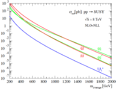
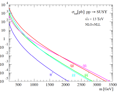
Figure 1: NLO+NLL cross sections for squark and gluino production at the LHC ($\sqrt{S}=8$ and 13 TeV). (The $\tilde{t}\tilde{t}^{*}$ curve in the lower plot corresponds to the $\tilde{t}_{1}\tilde{t}^{*}_{1}$ cross section; both notations $\tilde{q}^{*}$ and $\bar{\tilde{q}}$ are used in the literature to denote antisquarks.) The cross sections have been evaluated for a common squark and gluino mass $m_{\tilde{q}}=m_{\tilde{g}}=m_{\rm average}=m$, and the renormalization and factorization scales have been set to $\mu=m$. The MSTW2008 pdfs [67] have been used.

We observe that the inclusive cross section is dominated by $\tilde{q}\tilde{q}$ and $\tilde{q}\tilde{g}$ production at large sparticle masses, a consequence of the large valence quark component of the pdf at large $x$. Note that the $\tilde{q}\tilde{q}$, $\tilde{q}\tilde{g}$ and $\tilde{q}\bar{\tilde{q}}$ cross sections include the sum over five flavors of squarks, $\tilde{q}\in\{\tilde{u},\tilde{d},\tilde{c},\tilde{s},\tilde{b}\}$, and both chiralities ($\tilde{q}_{L}$ and $\tilde{q}_{R}$). Therefore, and because of a different threshold behaviour, the cross section for the production of light stops, $pp\to\tilde{t}_{1}\bar{\tilde{t}}_{1}$, is strongly suppressed.

The NLL summation increases the cross section prediction if the renormalization and factorization scales are chosen near the average mass of the final state particles. More importantly, threshold resummation leads to a significant reduction of the scale dependence over the full range of sparticle masses, with an overall scale uncertainty at NLO+NLL of less than 10%. This is shown in Fig. 2 for squark-gluino associated production. We also show the full theory uncertainty, consisting of the 68% C.L. pdf and $\alpha_{\rm s}$ error added in quadrature, combined linearly with the scale variation error for the NLO cross sections and for the NLO+NLL cross sections. We find that even though the pdf uncertainty is significant, the inclusion of threshold resummation leads to a sizeable reduction of the overall theory uncertainty.

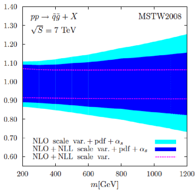
Figure 2: The theoretical uncertainty for associated squark-gluino production at the LHC with 7 TeV, $pp\to\tilde{q}\tilde{g}\,+X$, as a function of the sparticle mass $m_{\tilde{q}}=m_{\tilde{g}}=m$. The error bands represent the NLO+NLL scale uncertainty in the range $m/2\leq\mu\leq 2m$, and the total theory uncertainty including the 68% C.L. pdf and $\alpha_{\rm s}$ error, added in quadrature, and the error from scale variation in the range $m/2\leq\mu\leq 2m$ added linearly to the combined pdf and $\alpha_{\rm s}$ uncertainty. The total theory uncertainty is shown at both NLO and NLO+NLL. The MSTW2008 pdfs [67] have been used.

The NLO+NLL predictions for degenerate squark masses can be computed with the program Nll-fast [68] and are employed by the LHC experiments to interpret search limits and constrain the MSSM parameter space. Selected results for squark and gluino cross sections at current and future hadron colliders are collected in Refs. [51, 52], including a more detailed discussion of the theoretical scale and pdf uncertainty.

2.2 NNLL threshold resummation

Let us first briefly comment on the ingredients needed to extend the resummation of threshold logarithms to next-to-next-to-leading logarithmic accuracy. As discussed in Section 2.1, the (soft-)collinear radiation effects are described by the functions $\Delta_{i}$ and $\Delta_{j}$, while wide-angle soft radiation is accounted for by $\Delta^{\rm(s)}_{ij\to kl,I}$ in Eq. (5). The product of these radiative factors can be written schematically as

$$\Delta_{i}\Delta_{j}\Delta^{\rm(s)}_{ij\to kl,I}=$$ (7)

$$\exp\Big{[}Lg_{1}(\alpha_{\rm s}L)+g_{2}(\alpha_{\rm s}L)+\alpha_{\rm s}g_{3}(\alpha_{\rm s}L)+\ldots\Big{]}\,.$$

This exponent contains all the dependence on large logarithms $L=\ln N$. The leading logarithmic approximation (LL) is represented by the $g_{1}$ term alone, whereas the NLL approximation requires additionally including the $g_{2}$ term. Similarly, the $g_{3}$ term is needed for the NNLL approximation. The expressions for the $g_{1}$ and $g_{2}$ functions can be found in e.g. [35] and that for the NNLL $g_{3}$ function in e.g. [43].

The matching coefficients $C_{ij\to kl,I}$ in Eq. (5) collect non-logarithmic terms as well as logarithmic terms of non-soft origin in the Mellin moments of the higher-order contributions. The coefficients $C_{ij\to kl,I}$ factorise into a part that contains the Coulomb corrections and a part containing hard contributions [39]

$$C_{ij\to kl,I}=$$ (8)

$$(1+\frac{\alpha_{\rm s}}{\pi}{\cal C}_{ij\to kl,I}^{\rm Coul,(1)}+\frac{\alpha_{\rm s}^{2}}{\pi^{2}}{\cal C}_{ij\to kl,I}^{\rm Coul,(2)}+\dots)$$

$$\times (1+\frac{\alpha_{\rm s}}{\pi}{\cal C}_{ij\to kl,I}^{(1)}+\frac{\alpha_{\rm s}^{2}}{\pi^{2}}{\cal C}_{ij\to kl,I}^{(2)}+\dots)\,.$$

Apart from the terms of ${\cal O}(\alpha_{s})$, which need to be included in $C_{ij\to kl,I}$ when performing resummation at NNLL, some of the ${\cal O}(\alpha_{s}^{2})$ terms are also known and can be included in the numerical calculations. Expanding Eq. (8) we have

$$C^{\rm NNLL}_{ij\to kl,I}=$$ (9)

$$1+\frac{\alpha_{\rm s}}{\pi}\left({\cal C}^{\rm Coul,(1)}_{ij\to kl,I}+{\cal C}^{\rm(1)}_{ij\to kl,I}\right)$$

$$+\frac{\alpha_{\rm s}^{2}}{\pi^{2}}\left({\cal C}^{\rm Coul,(2)}_{ij\to kl,I}+{\cal C}^{\rm(2)}_{ij\to kl,I}+{\cal C}^{\rm(1)}_{ij\to kl,I}{\cal C}^{\rm Coul,(1)}_{ij\to kl,I}\right).$$

The first-order hard matching coefficients ${\cal C}^{\rm(1)}_{ij\to kl,I}$ were calculated in [49], whereas the expressions for the first-order Coulomb corrections ${\cal C}^{\rm Coul,(1)}_{ij\to kl,I}$ in Mellin-moment space are listed in [50]. The form of the two-loop Coulomb corrections in $x$-space is known in the literature [69], and the ${\cal C}^{\rm Coul,(2)}_{ij\to kl,I}$ coefficients have been calculated in [50] by taking Mellin moments of the near-threshold approximation of these two-loop Coulomb corrections. The second-order hard matching coefficient ${\cal C}^{\rm(2)}_{ij\to kl,I}$ is not known at the moment and we put ${\cal C}^{\rm(2)}_{ij\to kl,I}=0$ in Eq. (9).

Once we have the NNLL resummed cross section in Mellin-moment space, we match it to the approximated NNLO cross section, which is constructed by adding the near-threshold approximation of the NNLO correction [69] to the full NLO result [17]. The matching is performed according to

$$\sigma^{\rm(NNLL~{}matched)}_{h_{1}h_{2}\to kl}\bigl{(}\rho,\{m^{2}\},\mu^{2}\bigr{)}=\sigma^{\rm(NNLO_{Approx})}_{h_{1}h_{2}\to kl}\bigl{(}\rho,\{m^{2}\},\mu^{2}\bigr{)}$$ (10)

$$+\,\sum_{i,j}\,\int_{\mathrm{CT}}\,\frac{dN}{2\pi i}\,\rho^{-N}\,\tilde{f}_{i/h_{1}}(N+1,\mu^{2})\,\tilde{f}_{j/h_{2}}(N+1,\mu^{2})$$

$$\times\,\left[\tilde{\sigma}^{\rm(res,NNLL)}_{ij\to kl}\bigl{(}N,\{m^{2}\},\mu^{2}\bigr{)}\right.$$

$$\left.\,-\,\tilde{\sigma}^{\rm(res,NNLL)}_{ij\to kl}\bigl{(}N,\{m^{2}\},\mu^{2}\bigr{)}{\left.\right|}_{\scriptscriptstyle{\rm(NNLO_{Approx})}}\,\right].$$

To evaluate the inverse Mellin transform in Eq. (10) we again adopt the prescription of reference [66] for the integration contour CT.

In Fig. 3 we present the NNLL matched cross section prediction for the sum of the different squark and gluino production processes. The theoretical uncertainty includes the scale error as well as pdf and $\alpha_{\rm s}$ errors. It is obtained by linearly adding the scale dependence in the range $m/2\leq\mu\leq 2m$ to the combined 68% C.L. pdf and $\alpha_{\rm s}$ uncertainties, the latter two added in quadrature. We see uncertainties grow from approximately 5% for masses near the present lower bounds, to 10% for masses approaching 2.5 TeV. Including the NNLL contributions leads to a further reduction of the scale dependence for the squark and gluino production total cross sections, with the exception of gluino-pair production as discussed in more detail in Ref. [50].

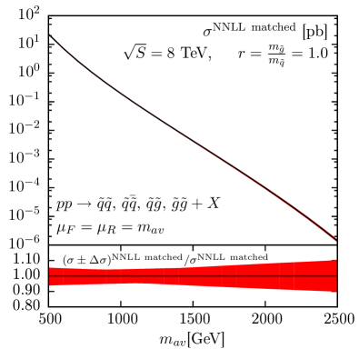
Figure 3: The NNLL matched cross section for the sum of the four processes of pair production of squarks and gluinos, including the theoretical error. The error band includes the 68% C.L. pdf and $\alpha_{\rm s}$ errors, added quadratically, and the scale uncertainty varied in the range $m_{av}/2\leq\mu\leq 2m_{av}$, added linearly to the combined pdf and $\alpha_{\rm s}$ error. The energy is that of the LHC at 8 TeV. The squark and gluino masses have been taken equal and the common renormalization and factorization scale has been set equal to the average mass of the two particles produced. The MSTW 2008 NNLO parton distribution function [67] has been used.

2.3 NLO-QCD corrections for generic MSSM spectra

The calculations implemented in Prospino and Nll-fast described in the previous section assume that five flavors of left- and right-chiral squarks, $\tilde{u}_{L,R}$, $\tilde{d}_{L,R}$, $\tilde{c}_{L,R}$, $\tilde{s}_{L,R}$, and $\tilde{b}_{L,R}$, are mass-degenerate. NLO-QCD predictions for generic MSSM spectra have been presented in the literature recently [53, 54, 55, 56, 57], and we shall briefly comment on these calculations below.

We shall follow Ref. [57] and discuss the production of squark-antisquark pairs as an example. General NLO squark and gluino production cross sections have also been presented in [54]. At LO squark-antisquark production, $pp\to\tilde{q}\bar{\tilde{q}}$, proceeds through quark-antiquark annihilation and gluon-fusion,

$$q_{i}\,\bar{q}_{j} \rightarrow\tilde{q}_{k}^{\,c1}\,\bar{\tilde{q}}_{l}^{\,c2}\,,$$ (11)

$$g\,g \rightarrow\tilde{q}_{i}^{\,c}\,\bar{\tilde{q}}_{i}^{\,c}\,.$$

Here, the lower indices indicate the flavor of the particle, whereas the upper indices for the squarks denote the chirality. Due to the flavor conserving structure of the relevant vertices the $gg$ initiated processes and the $s$-channel gluon exchange only contribute to the production of squarks of the same flavor and chirality. We shall focus on the production of squarks of the first two generations. In total, this includes 64 possible final state combinations. This number can be reduced to 36 independent channels if the invariance under charge conjugation is taken into account.

To illustrate the size of the SUSY-QCD corrections for the individual production channels, let us consider a particular benchmark scenario of the constrained MSSM  [70], specified by universal GUT-scale parameters $m_{0}/m_{1/2}/A_{0}=825/550/0$ GeV, $\tan(\beta)=10$ and $\text{sgn}(\mu)=+1$. The corresponding squark and gluino masses read

$m_{\tilde{u}_{L}}=m_{\tilde{c}_{L}}$​​	​​$m_{\tilde{u}_{R}}=m_{\tilde{c}_{R}}$ ​​​	​​​ $m_{\tilde{d}_{L}}=m_{\tilde{s}_{L}}$ ​​​​​	​​​ $m_{\tilde{d}_{R}}=m_{\tilde{s}_{R}}$ ​​​	​​ ​​ $m_{\tilde{g}}\!\!\!\!$
$\!\!1799.53\!\!$	$\!\!1760.21\!\!$	$\!\!1801.08\!\!$	$\!\!1756.40\!\!$	$\!\!1602.96\!\!$

where we have neglected the very small mass splitting between the first and second generation squarks.

In Table 1 we present LO and NLO results for individual squark-antisquark production channels at the LHC with 14 TeV. The renormalization and factorization scales have been set to the average squark mass, i.e. $\overline{m}_{\tilde{q}}=1779.31\,\text{GeV}$, and the CTEQ6L1 [71] and CT10NLO [72] parton distribution functions have been adopted for the LO and NLO cross sections, respectively.

Process	$\sigma_{\text{LO}}[\text{fb}]$	$\sigma_{\text{NLO}}[\text{fb}]$	K-factor
$\tilde{u}_{L}\bar{\tilde{u}}_{L}$	$9.51\cdot 10^{-2}$	$1.43\cdot 10^{-1}$	$1.50$
$\tilde{u}_{R}\bar{\tilde{u}}_{R}$	$1.14\cdot 10^{-1}$	$1.72\cdot 10^{-1}$	$1.51$
$\tilde{d}_{L}\bar{\tilde{d}}_{L}$	$5.50\cdot 10^{-2}$	$8.79\cdot 10^{-2}$	$1.60$
$\tilde{d}_{R}\bar{\tilde{d}}_{R}$	$6.89\cdot 10^{-2}$	$1.11\cdot 10^{-1}$	$1.61$
$\tilde{u}_{L}\bar{\tilde{u}}_{R}$	$3.75\cdot 10^{-1}$	$5.12\cdot 10^{-1}$	$1.37$
$\tilde{d}_{L}\bar{\tilde{d}}_{R}$	$1.41\cdot 10^{-1}$	$1.70\cdot 10^{-1}$	$1.21$
$\tilde{u}_{L}\bar{\tilde{d}}_{L}$	$6.98\cdot 10^{-2}$	$7.89\cdot 10^{-2}$	$1.13$
$\tilde{u}_{L}\bar{\tilde{d}}_{R}$	$2.98\cdot 10^{-1}$	$3.54\cdot 10^{-1}$	$1.19$
$\tilde{u}_{R}\bar{\tilde{d}}_{L}$	$2.94\cdot 10^{-1}$	$3.49\cdot 10^{-1}$	$1.19$
$\tilde{u}_{R}\bar{\tilde{d}}_{R}$	$8.36\cdot 10^{-2}$	$9.54\cdot 10^{-2}$	$1.14$
Sum	1.59	2.07	1.30

Table 1: The LO and NLO cross sections for squark-antisquark production of the first generation at the LHC with $\sqrt{S}=14$ TeV obtained for a specific scenario of the constrained MSSM as described in the text. The renormalization and factorization scales have been set to the average squark mass, i.e. $\overline{m}_{\tilde{q}}=1779.31\,\text{GeV}$, and the CTEQ6L1 [71] and CT10NLO [72] parton distribution functions have been adopted for the LO and NLO cross sections, respectively.

Note, that the channels with squarks of the same flavor and chirality in the final state, displayed in the first four rows of the table, have contributions from $gg$ initial states and therefore larger $K$-factors than channels with squarks of different flavor or chirality. Hence, approximating the individual $K$-factors by the average $K$-factor as obtained from Prospino, $K_{\rm avg}=1.39$, is not very accurate .

Determining the individual corrections consistently is especially important if the decays are taken into account and the branching ratios of the different squarks differ significantly for the specific decay channel under consideration. In order to assess the possible numerical impact of this approximation we consider the decay $\tilde{q}\rightarrow q\tilde{\chi}^{0}_{1}$ at LO at the level of total cross sections, i.e. we multiply the production cross sections for the individual squark-antisquark channels with the respective LO branching ratios:

$$\sum_{\text{channels}}\sigma_{\text{NLO}}\cdot\text{BR}^{\text{LO}}\left(\tilde{q}\rightarrow\tilde{\chi}^{0}_{1}q\right)\cdot\text{BR}^{\text{LO}}\left(\bar{\tilde{q}}\rightarrow\tilde{\chi}^{0}_{1}\bar{q}\right)$$ (12)

$$=0.139\,\text{fb}.$$

Multiplying the LO result for each subchannel with the average $K$-factor, $K_{\rm avg}=1.39$, and the corresponding branching ratios gives

$$\sum_{\text{channels}}\sigma_{\text{LO}}\cdot K^{\text{avg}}\cdot\text{BR}^{\text{LO}}\left(\tilde{q}\rightarrow\tilde{\chi}^{0}_{1}q\right)\cdot\text{BR}^{\text{LO}}\left(\bar{\tilde{q}}\rightarrow\tilde{\chi}^{0}_{1}\bar{q}\right)$$ (13)

$$=0.126\,\text{fb}\,.$$

Thus the rate obtained with the approximation relying on an average $K$-factor for all subchannels is roughly $10\%$ smaller for this particular case.

To summarize this section, we have seen that using an average $K$-factor to globally rescale individual sub-channels for squark-antisquark production may not be a very accurate approximation. For a generic benchmark scenario, we find differences of $\mathcal{O}(10\%)$, i.e. of phenomenological relevance for the experimental accuracy expected in run 2 of the LHC. In general, the more the branching ratios of the different squarks differ, the more important the consistent treatment of the individual corrections becomes.

3 Light stop decays

Higher-order QCD corrections to supersymmetric particle decay widths and branching ratios have been calculated for many years, see e.g. Ref. [73, 74] and references therein. Here, we shall focus on the decays of light stops, which play a special role in supersymmetric models.

In most SUSY models a light stop arises naturally, as the mixing is proportional to the large top Yukawa coupling, which leads to a large mass splitting between the stop mass eigenstates. Light stops play an important role in view of the Higgs mass and naturalness arguments; together with the top loops they provide the dominant higher-order corrections to the light CP-even Higgs mass [75, 76, 77, 78, 79], which are necessary to shift the tree-level mass to the observed value of about 125 GeV. A light stop can also lead to the correct dark matter relic density through co-annihilation, in particular for mass differences between the stop and the lightest neutralino $\tilde{\chi}_{1}^{0}$ of 15-30 GeV [80, 81, 82, 83, 84, 85]. Moreover, light stops allow for successful baryogenesis within the MSSM [86, 87, 88, 89, 90, 91, 92, 93, 94, 95, 96, 97, 98].

While the canonical LHC searches for jets and missing transverse energy place lower limits on the masses of the squarks of the first two generations of approximately 1.5 TeV [12, 13], the lightest stop can still be rather light and have a mass below the kinematical threshold for the decay into a top quark and the lightest neutralino $\tilde{\chi}_{1}^{0}$. If we assume the lightest stop $\tilde{t}_{1}$ to be the next-to-lightest SUSY particle (NLSP) and the lightest neutralino to be the lightest SUSY particle, then $\tilde{t}_{1}$ can decay into the LSP and a charm quark $c$ or an up quark $u$, i.e. $\tilde{t}_{1}\to(u/c)\,\tilde{\chi}_{1}^{0}$ [99, 100]. Another possible decay channel is the four-body decay $\tilde{t}_{1}\to\tilde{\chi}_{1}^{0}bf\bar{f}^{\prime}$ [101], where $f$ and $f^{\prime}$ denote generic light fermions. The two-body decay into charm/up and neutralino is flavor-violating (FV). While the MSSM in general exhibits many sources of flavor violation, so that the decay can already occur at tree-level, high precision tests in the sector of quark flavor violation and limits on flavor-violating neutral currents from $K$, $D$ and $B$ meson studies put stringent constraints on the amount of possible flavor violation. The hypothesis of Minimal Flavor Violation (MFV) [102, 103, 104, 105, 106] has been proposed in order to solve this New Physics Flavor Puzzle. It requires that all sources of flavor and CP-violation are given by the SM structure of the Yukawa couplings, so that flavor mixing in models of New Physics is then always proportional to the off-diagonal elements of the Cabibbo-Kobayashi-Maskawa (CKM) matrix [107, 108]. However, the hypothesis of MFV is not renormalization group invariant [105]. Flavor off-diagonal squark mass terms are induced through the Yukawa couplings, so that the squark and quark mass matrices cannot be diagonalized simultaneously any more and e.g. the stop state receives some admixture from the charm (up) squark, inducing a tree-level flavor-changing neutral current (FCNC) coupling between the stop, the lightest neutralino and the charm (up) quark. Note that for very small FV stop-neutralino-up/charm quark couplings, the four-body decay can become important and has to be considered for a reliable prediction of the $\tilde{t}_{1}$ branching ratios. The stop masses have been bounded by LEP [109, 110] and Tevatron [111, 112], and more recently by ATLAS [113] and CMS [114], with the strongest limits coming from the ATLAS analyses Refs. [115, 116]. All these analyses assume a branching ratio equal to one for the considered decay channel of the $\tilde{t}_{1}$, i.e. either the FV two-body or the four-body decay. The branching ratios, however, can deviate significantly from one in large parts of the allowed parameter range, as has been shown in Refs. [100, 117] and will be outlined in the following. Taking this effect into account, the experimental exclusion limits on the stop, which are based on the assumption of branching ratios equal to one, are considerably weakened.

In Ref. [100] we improved upon the existing approximate result for the $\tilde{t}_{1}\to(u/c)\,\tilde{\chi}_{1}^{0}$ decay of Ref. [99], which only takes into account the leading logarithms of the MFV scale. We calculated the exact one-loop decay width in the framework of MFV, by performing the full renormalization program and including the finite non-logarithmic terms arising from the loop integrals. For the numerical analysis we investigated two constrained MSSM scenarios with universal soft-breaking terms at the GUT scale $M_{\rm GUT}\approx 10^{16}$ GeV. This scale is identified with the MFV scale, and all soft SUSY breaking parameters are family universal. The boundary conditions at $\mu_{\mbox{\scriptsize MFV}}=M_{\rm GUT}$ are

$$\begin{array}[]{lll}(1)&m_{0}=200\mbox{ GeV};&m_{1/2}=230\mbox{ GeV};\\ A_{0}=-920\mbox{ GeV};&\tan\beta=10;&\mbox{sign}(\mu)=+;\\[5.69054pt] (2)&m_{0}=200\mbox{ GeV};&m_{1/2}=230\mbox{ GeV};\\ A_{0}=-895\mbox{ GeV};&\tan\beta=10;&\mbox{sign}(\mu)=+.\\ \end{array}$$ (18)

The mass spectra and mixing angles have been calculated with the spectrum calculator SPheno [118, 119], which allows for flavor violation. The second scenario has a larger $\tilde{t}_{1}-\tilde{\chi}_{1}^{0}$ mass difference compared to scenario (1), whereas the mass difference between $\tilde{t}_{1}$ and the lightest chargino $\tilde{\chi}_{1}^{+}$ is smaller:

$$\begin{array}[]{llll}(1)&m_{\tilde{t}_{1}}/m_{\tilde{\chi}_{1}^{0}}/m_{\tilde{\chi}_{1}^{+}}=104/92/175\mbox{ GeV};\\ (2)&m_{\tilde{t}_{1}}/m_{\tilde{\chi}_{1}^{0}}/m_{\tilde{\chi}_{1}^{+}}=130/92/175\mbox{ GeV}.\end{array}$$ (21)

The partial stop decay width into charm and neutralino has been calculated with the full one-loop formula and compared to the approximate result [99]. For the latter, the charged $W$ boson mass $M_{W}$ has been taken as generic loop particle mass. The widths are given in Table 2.

$\begin{array}[]{c|c|c}\tilde{t}_{1}\to c\tilde{\chi}_{1}^{0}&\Gamma^{\mbox{\scriptsize{1-loop}}}\mbox{[GeV]}&\Gamma^{\mbox{\scriptsize{H/K}}}\mbox{[GeV]}\\ \hline\cr\mbox{Scenario}\,(1)&9.322\cdot 10^{-10}&1.004\cdot 10^{-9}\\ \hline\cr\mbox{Scenario}\,(2)&5.862\cdot 10^{-9}&6.446\cdot 10^{-9}\\ \end{array}$

Table 2: The partial widths for the decay $\tilde{t}_{1}\to c\tilde{\chi}_{1}^{0}$ in two MFV scenarios, calculated with the exact 1-loop formula, $\Gamma^{\mbox{\scriptsize{1-loop}}}$, and with the approximate formula of Ref. [99], $\Gamma^{\mbox{\scriptsize{H/K}}}$.

They have been obtained with the program Susy-Hit [73, 74], where the full one-loop formula for the flavor changing stop decay has been implemented. The results for the exact and the approximate decay widths differ by ${\cal O}(10\%)$. In the calculation of the branching ratios the $\tilde{t}_{1}\to u\tilde{\chi}_{1}^{0}$ and the four-body decay widths have also been included in the total width. The branching ratios are summarised in Table 3. In scenario (2) the larger mass difference between $\tilde{t}_{1}$ and $\tilde{\chi}_{1}^{0}$ leads to a more important four-body decay width, as it is dominated by the chargino exchange diagrams [101]. This in turn induces a deviation of the branching ratio $\mbox{BR}(\tilde{t}_{1}\to\tilde{\chi}_{1}^{0}c)$ from one by a few per-cent, as can be inferred from Table 3.

$\begin{array}[]{c|c|c}\mbox{BR}&\mbox{BR}(\tilde{t}_{1}\to\tilde{\chi}_{1}^{0}c)&\mbox{BR}(\tilde{t}_{1}\to\tilde{\chi}_{1}^{0}bf\bar{f}^{\prime})\\ \hline\cr\mbox{Scenario}\,(1)&0.9944&4.587\cdot 10^{-5}\\ \hline\cr\mbox{Scenario}\,(2)&0.9443&0.0504\end{array}$

Table 3: The $\tilde{t}_{1}$ branching ratios for different final states for scenario (1) and (2). For details, see [100].

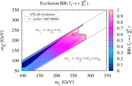
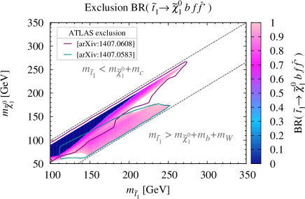
Figure 4: Exclusion limits in the $m_{\tilde{\chi}_{1}^{0}}-m_{\tilde{t}_{1}}$ plane at 95% CL, based on the results for the $\tilde{t}_{1}\to c\tilde{\chi}_{1}^{0}$ signature from [115] (left) and on the results for the $\tilde{t}_{1}\to\tilde{\chi}_{1}^{0}bf\bar{f}^{\prime}$ signature from [115, 116] (right). The color code indicates the branching ratio down to which the exclusion limits are valid. Taken from [117].

For MFV scales large compared to the EWSB scale, the two-body decay width is dominated by large logarithms of the ratios of these scales, which should be resummed. Resummation effects can be included by taking into account the FCNC couplings that are induced through renormalization group running already at tree-level. This has been done in Ref. [117] where we calculated the one-loop SUSY-QCD corrections to the two-body decay. For the correct determination of the $\tilde{t}_{1}$ branching ratios, also the four-body decay is computed by consistently including FCNC couplings. Furthermore, non-vanishing masses for the third generation fermions in the final state have been taken into account. These decay widths have been implemented in Susy-Hit [73, 74]. (The program with the newly implemented stop decays is available at [120].) The improved $\tilde{t}_{1}$ branching ratios have implications for the LHC stop searches and the bounds obtained on the mass of the lightest stop $m_{\tilde{t}_{1}}$. To show this we have performed a parameter scan and taken care to respect constraints from Higgs data, SUSY searches, $B$-physics measurements and from the relic density. For details, we refer to [117]. Figure 4 shows the exclusion limits on $m_{\tilde{t}_{1}}$ depending on the mass $m_{\tilde{\chi}_{1}^{0}}$, taking into account our results, i.e. as a function of the actual value of the $\tilde{t}_{1}$ branching ratio. The plot reinterprets the ATLAS searches based on monojet-like [115] and charm-tagged event selections [115] and on searches for final states with one isolated lepton, jets and missing transverse momentum [116], where limits on the lightest stop mass as a function of the neutralino mass have been given, assuming a branching ratio of one. The grey dashed lines in the figure limit the region in which $m_{\tilde{\chi}_{1}^{0}}+m_{c}\leq m_{\tilde{t}_{1}}\leq m_{\tilde{\chi}_{1}^{0}}+m_{b}+m_{W}\;.$ In this region the stop can be searched for in the FV two-body decay and the four-body decay. The full pink line in the upper plot is the 95% CL exclusion limit based on combined charm-tagged and monojet ATLAS searches in the $\tilde{t}_{1}\to c\tilde{\chi}_{1}^{0}$ decay [115], assuming a branching ratio of one. Under the assumption that $\tilde{t}_{1}$ decays exclusively into the four-body final state, ATLAS derived from the monojet analysis [115] the exclusion given by the pink line (close to the upper dashed line) in Fig. 4 (right) and from the final states with one isolated lepton the exclusion region delineated by the green line (close to the lower dashed line) [116]. With the information given in [115, 116] we derived the exclusion limits for the two- and the four-body final state as a function of the branching ratio, which is given by the color code.

The plot shows the stop masses that are excluded for a branching ratio above the one associated with a specific color. Evidently, for smaller branching ratios the exclusion limits become weaker. The combination of the two plots allows to extract the exclusion limits for stops of a given mass as function of the neutralino mass and the stop branching ratio. Thus it can be read off from Fig. 4 (left) that $\tilde{t}_{1}$ masses of 150 GeV can be excluded for $m_{\tilde{\chi}_{1}^{0}}=80$ GeV if their branching ratio into $c+\tilde{\chi}_{1}^{0}$ exceeds $0.43$. This in turn implies that the stop four-body branching ratio is below 0.57. On the other hand the right plot shows that in the same region stops can be excluded if their branching ratio into the four-body final state is larger than 0.88, which implies that the two-body decay branching ratio is below 0.12 then. This means that $m_{\tilde{t}_{1}}=150$ GeV can be excluded for $m_{\tilde{\chi}_{1}^{0}}=80$ GeV for scenarios in which $\mbox{BR}(\tilde{t}_{1}\to c\tilde{\chi}_{1}^{0})<0.12$ and $\mbox{BR}(\tilde{t}_{1}\to c\tilde{\chi}_{1}^{0})>0.43$, respectively, $\mbox{BR}(\tilde{t}_{1}\to\tilde{\chi}_{1}^{0}bf\bar{f}^{\prime})>0.88$ and $\mbox{BR}(\tilde{t}_{1}\to\tilde{\chi}_{1}^{0}bf\bar{f}^{\prime})<0.57$. The dark blue regions correspond to stops with vanishing branching ratios, so that all stop mass values associated with these regions are excluded. In Fig. 4 (left) there is no smooth transition between the dark blue and its neighbouring regions, as the exclusion limits in the two-body final state are related to the ones in the four-body final state which here apply for branching ratios $\gtrsim 0.46$, so that of course also in Fig. 4 (right) there is no continuous color gradient.

The exclusion limits given by the border of the colored region at 100% two-, respectively, four-body decay branching ratio, do not exactly match the ones derived by ATLAS. The reason is that ATLAS provided information on the values of the excluded production cross section times branching ratio only for a few points in the $m_{\tilde{\chi}_{1}^{0}}-m_{\tilde{t}_{1}}$ plane so that a linear interpolation between these points was necessary in order to cover the whole region. Nevertheless, the agreement of the presented results with the given exclusion limits is reasonably good. The advantage of our approach is that it takes properly into account the information on the actual stop branching ratios which can considerably weaken the stop exclusion limits as is evident from Fig. 4. As these plots can only be an approximation of what can be done much more accurately by the experiments, they should be taken as an encouragement to provide results also as function of the stop branching ratios.

4 Exclusive squark production and decay at the LHC

Fully differential NLO calculations of squark and gluino production and decay have been presented recently  [53, 55, 56, 57, 121, 122], including the matching to parton showers for squark-squark and squark-antisquark production [55, 57]. These calculations show that higher-order QCD effects may significantly modify the shape of differential distributions. Thus, leading-order Monte-Carlo predictions scaled with inclusive QCD corrections do, in general, not provide an accurate description of exclusive observables and cross sections with kinematic cuts. We shall discuss the impact of the higher-order corrections on the differential distributions following the analysis of squark-antisquark and squark-squark production presented in Ref. [57].

In order to quantify the impact of the parton shower on the differential distributions, we have matched the NLO-calculation presented in Section 2.3 with various parton shower showers using the matching scheme of Ref. [123] as implemented in the Powheg-Box [124]. The corresponding code is publicly available and can be downloaded at [125].

Let us first comment on the impact of the NLO corrections on the shape of the differential distributions. We consider the production of a squark-antisquark pair, $pp\to\tilde{q}\bar{\tilde{q}}$, followed by (anti-)squark decay into a neutralino and a jet, $\tilde{q}/\bar{\tilde{q}}\rightarrow q/\bar{q}\,\tilde{\chi}^{0}_{1}$. In Fig. 5 we present the LO and the NLO distributions for the transverse momentum of the hardest jet, $p_{T}^{j_{1}}$, using the benchmark scenario described in Section 2.3 (see Ref. [57] for details). One observes a strong enhancement of the NLO corrections for small values of $p_{T}$, while they turn even negative for large values. The result for the second hardest jet, which is not shown here, is qualitatively the same.

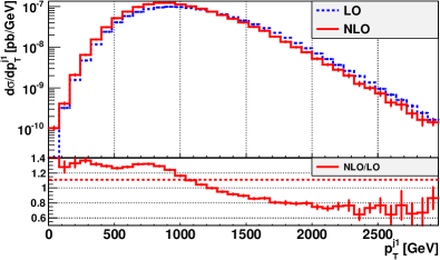
Figure 5: Transverse momentum distribution of the hardest jet, $p_{T}^{j_{1}}$, for squark production at the LHC ($\sqrt{S}=14$ TeV), combined with the subsequent (anti-)squark decay $\tilde{q}/\bar{\tilde{q}}\rightarrow q/\bar{q}\,\tilde{\chi}^{0}_{1}$ for the SUSY scenario described in the text. Shown are the LO and NLO results, as well as the differential $K$-factor (full) and the total $K$-factor (dashed).

More accurate predictions for differential distributions and exclusive observables require the matching of the NLO calculations with a parton shower. We have followed the matching scheme presented in Ref. [123] and implemented the NLO SUSY-QCD calculation of $pp\to(\tilde{q}\to q\tilde{\chi}^{0}_{1})(\bar{\tilde{q}}\to\bar{q}\tilde{\chi}^{0}_{1})+X$ into the Powheg-Box [124]. We have compared the default Pythia 6 [126] and Herwig++ [127] parton showers, and a $p_{T}$-ordered dipole shower [128, 129], which is also implemented in Herwig++. We find that the predictions of the different parton showers for the observables depending solely on the two hardest jets agree within ${\cal O}(10\%)$ or better. Comparing the showered results with the outcome of a pure NLO simulation the effects of the parton showers on these observables are at most of ${\cal O}(20\%)$, except for the threshold region. Larger deviations between the different parton showers emerge in the predictions for the third hardest jet, which is formally described only at LO in the hard process, see Fig. 6.

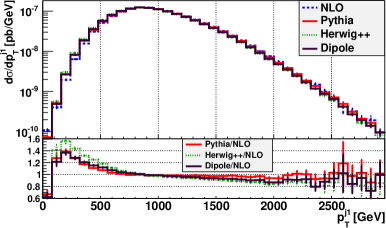
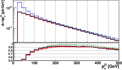
Figure 6: Transverse momentum distribution of the hardest (upper panel) and third hardest (lower panel) jet, for squark production at the LHC ($\sqrt{S}=14$ TeV), combined with the subsequent (anti-)squark decay $\tilde{q}/\bar{\tilde{q}}\rightarrow q/\bar{q}\,\tilde{\chi}^{0}_{1}$ for the SUSY scenario described in the text. The NLO predictions and the NLO results matched to the parton showers Pythia [126], Herwig++ [127] and the Dipole-Shower [128, 129], are shown. The lower inserts depict the respective ratios of the results obtained with the three parton showers and the pure NLO prediction.

Let us finally comment on the impact of the higher-order corrections on event rates after experimental selection cuts. We consider the definition of a signal region for the SUSY searches in two-jet events performed by the ATLAS collaboration [130] with event selection cuts corresponding to

$$p_{T}^{j_{1}}>130\,\text{GeV},\quad p_{T}^{j_{2}}>60\,\text{GeV},\quad\not{E}_{T}>160\,\text{GeV},$$

$$\ \frac{\not{E}_{T}}{m_{\text{eff}}}>0.2,\quad m_{\text{eff}}^{\text{incl}}>1\,\text{TeV},\quad\Delta\phi(j_{1/2},\vec{\not{E}}_{T})>0.4,$$

$$\quad\mbox{and}\;\;\Delta\phi(j_{3},\vec{\not{E}}_{T})>0.4\,\,\,\,\,\text{if}\,\,\,\,\,p_{T}^{j_{3}}>40\,\text{GeV}\,.$$ (22)

Here, the effective mass $m_{\text{eff}}$ is defined as the sum of the $p_{T}$ of the two hardest jets and $\not{E}_{T}$, whereas the inclusive definition of this observable includes all jets with $p_{T}^{j}>40\,\text{GeV}$,

$$m_{\text{eff}}^{\text{incl}}=\sum_{i=1}^{n_{j}}p_{T}^{j_{i}}+\not{E}_{T}\,.$$ (23)

Moreover, $\Delta\phi(j_{i},\vec{\not{E}}_{T})$ denotes the minimal azimuthal separation between the direction of the missing transverse energy, $\vec{\not{E}}_{T}$, and the $i^{\text{th}}$ jet. The additional cut $\Delta\phi(j_{3},\vec{\not{E}}_{T})>0.4$ is only applied if a third jet with $p_{T}^{j_{3}}>40\,\text{GeV}$ is present.

	$\tilde{q}\tilde{q}$	$\tilde{q}\bar{\tilde{q}}$
NLO	$0.871\,\text{fb}$	$0.0781\,\text{fb}$
Pythia	$0.883\,\text{fb}$	$0.0797\,\text{fb}$
Herwig++	$0.895\,\text{fb}$	$0.0807\,\text{fb}$

Table 4: Total cross sections after applying the event selection cuts defined in Eq. (22) for squark-squark and squark-antisquark production and subsequent decay $\tilde{q}\rightarrow q\tilde{\chi}^{0}_{1}$ within the benchmark scenario introduced in Section 2.3 and specified in detail in Ref. [57]. Results have been obtained at the level of a pure NLO simulation and including parton shower effects with Pythia and Herwig++, respectively.

Applying these cuts at the level of a pure NLO simulation yields the event rates as shown in the first row of Tab. 4. Results are shown for squark-squark and squark-antisquark production and subsequent decay $\tilde{q}\rightarrow q\tilde{\chi}^{0}_{1}$ within the benchmark scenario introduced in Section 2.3 and specified in detail in Ref. [57]. Matching these NLO results with a parton shower hardly affects the outcome after using the cuts defined in Eq. (22), as can be inferred from the results obtained with Pythia and the Herwig++ default shower listed in the second and third row, respectively.

To conclude, we have discussed the effect of matching various parton showers to a NLO-QCD calculation of squark-squark and squark-antisquark production. We find moderate shower effects of at most of ${\cal O}(10-20\%)$ for the observables depending solely on the two hardest jets, or for rather inclusive observables like event rates with selection cuts. In more exclusive distributions, including for example those for subleading jets, the effect of the parton shower may be more sizeable.

5 Conclusions

Supersymmetric theories are among the most attractive extensions of the Standard Model, and searches for SUSY play a key role in the LHC physics program. A tremendous amount of work has been done in the last 20 years to calculate higher-order corrections to the production and decay of supersymmetric particles at hadron colliders. Such precision calculations are important to place limits on the masses of supersymmetric particles from current and future LHC searches, and they will be essential to determine the parameters of a supersymmetric theory in the case of discovery at the upcoming LHC run 2.

The production cross sections for the strongly interacting SUSY particles, squarks and gluinos, are known at next-to-leading order in SUSY-QCD, including the summation of threshold logarithms at next-to-next-to-leading accuracy. The uncertainty of the theoretical predictions is at a level of $\lesssim 15\%$ and dominated by the error on the parton distribution functions. Similarly, there is a vast literature on higher-order corrections to SUSY particle decay widths and branching ratios, covering most of the relevant decay modes in the MSSM.

To fully exploit the potential of the LHC run 2, it is crucial to obtain precise predictions for more exclusive observables, including differential distributions and cross sections with cuts. To this end, one needs to consider higher-order corrections to SUSY particle production and decay chains, and to match the NLO predictions with parton showers. First results of such a more comprehensive analysis have been presented here.

Finally, future work should focus on developing automated tools to extend precision calculations to a wider class of beyond the SM physics scenarios. Such tools need to combine next-to-leading order accuracy in QCD for generic beyond the SM processes with the summation of large logarithmic threshold corrections and the matching with parton shower Monte Carlo programs.

References

- [1] J. Wess and B. Zumino, “Supergauge Transformations in Four-Dimensions,” Nucl. Phys. B 70 (1974) 39.
- [2] P. Langacker and M. X. Luo, “Implications of precision electroweak experiments for , , and grand unification,” Phys. Rev. D 44 (1991) 817.
- [3] U. Amaldi, W. de Boer and H. Furstenau, “Comparison of grand unified theories with electroweak and strong coupling constants measured at LEP,” Phys. Lett. B 260 (1991) 447.
- [4] J. R. Ellis, S. Kelley and D. V. Nanopoulos, “Probing the desert using gauge coupling unification,” Phys. Lett. B 260 (1991) 131.
- [5] E. Gildener, “Gauge Symmetry Hierarchies,” Phys. Rev. D 14 (1976) 1667.
- [6] M. J. G. Veltman, “The Infrared - Ultraviolet Connection,” Acta Phys. Polon. B 12 (1981) 437.
- [7] R. Barbieri and G. F. Giudice, “Upper Bounds on Supersymmetric Particle Masses,” Nucl. Phys. B 306 (1988) 63.
- [8] P. Fayet, “Spontaneously Broken Supersymmetric Theories of Weak, Electromagnetic and Strong Interactions,” Phys. Lett. B 69 (1977) 489.
- [9] G. R. Farrar and P. Fayet, “Phenomenology of the Production, Decay, and Detection of New Hadronic States Associated with Supersymmetry,” Phys. Lett. B 76 (1978) 575.
- [10] H. Goldberg, “Constraint on the Photino Mass from Cosmology,” Phys. Rev. Lett. 50 (1983) 1419 [Erratum-ibid. 103 (2009) 099905].
- [11] J. R. Ellis, J. S. Hagelin, D. V. Nanopoulos, K. A. Olive and M. Srednicki, “Supersymmetric Relics from the Big Bang,” Nucl. Phys. B 238 (1984) 453.
- [12] G. Aad et al. [ATLAS Collaboration], “Search for direct pair production of the top squark in all-hadronic final states in proton-proton collisions at TeV with the ATLAS detector,” JHEP 1409 (2014) 015 [arXiv:1406.1122 [hep-ex]].
- [13] S. Chatrchyan et al. [CMS Collaboration], “Search for new physics in the multijet and missing transverse momentum final state in proton-proton collisions at = 8 TeV,” JHEP 1406 (2014) 055 [arXiv:1402.4770 [hep-ex]].
- [14] H. P. Nilles, “Supersymmetry, Supergravity and Particle Physics,” Phys. Rept. 110 (1984) 1.
- [15] H. E. Haber and G. L. Kane, “The Search for Supersymmetry: Probing Physics Beyond the Standard Model,” Phys. Rept. 117 (1985) 75.
- [16] J. R. Ellis and S. Rudaz, “Search For Supersymmetry In Toponium Decays,” Phys. Lett. B 128, 248 (1983).
- [17] W. Beenakker, R. Höpker, M. Spira and P. M. Zerwas, “Squark and gluino production at hadron colliders,” Nucl. Phys. B 492, 51 (1997) [hep-ph/9610490].
- [18] W. Beenakker, M. Krämer, T. Plehn, M. Spira and P. M. Zerwas, “Stop production at hadron colliders,” Nucl. Phys. B 515, 3 (1998) [hep-ph/9710451].
- [19] W. Beenakker, M. Klasen, M. Krämer, T. Plehn, M. Spira and P. M. Zerwas, “The Production of charginos / neutralinos and sleptons at hadron colliders,” Phys. Rev. Lett. 83, 3780 (1999) [Erratum-ibid. 100, 029901 (2008)] [hep-ph/9906298].
- [20] E. L. Berger, M. Klasen and T. M. P. Tait, “Next-to-leading order SUSY QCD predictions for associated production of gauginos and gluinos,” Phys. Rev. D 62, 095014 (2000) [hep-ph/0005196].
- [21] E. L. Berger, M. Klasen and T. M. P. Tait, “Erratum: Next-to-leading order supersymmetric QCD predictions for associated production of gauginos and gluinos (Phys.Rev.D62:095014,2000),” Phys. Rev. D 67, 099901 (2003) [hep-ph/0212306].
- [22] S. Bornhauser, M. Drees, H. K. Dreiner and J. S. Kim, “Electroweak contributions to squark pair production at the LHC”, Phys. Rev. D 76 (2007) 095020 [arXiv:0709.2544 [hep-ph]].
- [23] W. Hollik, M. Kollar and M. K. Trenkel, “Hadronic production of top-squark pairs with electroweak NLO contributions,” JHEP 0802, 018 (2008) [arXiv:0712.0287 [hep-ph]].
- [24] M. Beccaria, G. Macorini, L. Panizzi, F. M. Renard and C. Verzegnassi, “Stop-antistop and sbottom-antisbottom production at LHC: A One-loop search for model parameters dependence,” Int. J. Mod. Phys. A 23, 4779 (2008) [arXiv:0804.1252 [hep-ph]].
- [25] W. Hollik and E. Mirabella, “Squark anti-squark pair production at the LHC: The Electroweak contribution,” JHEP 0812, 087 (2008) [arXiv:0806.1433 [hep-ph]].
- [26] W. Hollik, E. Mirabella and M. K. Trenkel, “Electroweak contributions to squark-gluino production at the LHC,” JHEP 0902, 002 (2009) [arXiv:0810.1044 [hep-ph]].
- [27] E. Mirabella, “NLO electroweak contributions to gluino pair production at hadron colliders,” JHEP 0912, 012 (2009) [arXiv:0908.3318 [hep-ph]].
- [28] A. Arhrib, R. Benbrik, K. Cheung and T. -C. Yuan, “Higgs boson enhancement effects on squark-pair production at the LHC,” JHEP 1002, 048 (2010) [arXiv:0911.1820 [hep-ph]].
- [29] J. Germer, W. Hollik, E. Mirabella and M. K. Trenkel, “Hadronic production of squark-squark pairs: The electroweak contributions,” JHEP 1008, 023 (2010) [arXiv:1004.2621 [hep-ph]].
- [30] J. Germer, W. Hollik and E. Mirabella, “Hadronic production of bottom-squark pairs with electroweak contributions,” JHEP 1105, 068 (2011) [arXiv:1103.1258 [hep-ph]].
- [31] J. Germer, W. Hollik, J. M. Lindert and E. Mirabella, “Top-squark pair production at the LHC: a complete analysis at next-to-leading order,” JHEP 1409 (2014) 022 [arXiv:1404.5572 [hep-ph]].
- [32] W. Beenakker, R. Hopker and M. Spira, “PROSPINO: A Program for the production of supersymmetric particles in next-to-leading order QCD,” hep-ph/9611232.
- [33] A. Kulesza and L. Motyka, “Threshold resummation for squark-antisquark and gluino-pair production at the LHC,” Phys. Rev. Lett. 102, 111802 (2009) [arXiv:0807.2405 [hep-ph]].
- [34] U. Langenfeld and S.-O. Moch, “Higher-order soft corrections to squark hadro-production,” Phys. Lett. B 675, 210 (2009) [arXiv:0901.0802 [hep-ph]].
- [35] A. Kulesza and L. Motyka, “Soft gluon resummation for the production of gluino-gluino and squark-antisquark pairs at the LHC,” Phys. Rev. D 80, 095004 (2009) [arXiv:0905.4749 [hep-ph]].
- [36] M. Beneke, P. Falgari and C. Schwinn, “Soft radiation in heavy-particle pair production: All-order colour structure and two-loop anomalous dimension,” Nucl. Phys. B 828, 69 (2010) [arXiv:0907.1443 [hep-ph]].
- [37] W. Beenakker, S. Brensing, M. Krämer, A. Kulesza, E. Laenen and I. Niessen, “Soft-gluon resummation for squark and gluino hadroproduction,” JHEP 0912, 041 (2009) [arXiv:0909.4418 [hep-ph]].
- [38] W. Beenakker, S. Brensing, M. Krämer, A. Kulesza, E. Laenen and I. Niessen, “Supersymmetric top and bottom squark production at hadron colliders,” JHEP 1008, 098 (2010) [arXiv:1006.4771 [hep-ph]].
- [39] M. Beneke, P. Falgari and C. Schwinn, “Threshold resummation for pair production of coloured heavy (s)particles at hadron colliders,” Nucl. Phys. B 842, 414 (2011) [arXiv:1007.5414 [hep-ph]].
- [40] W. Beenakker, S. Brensing, M. Krämer, A. Kulesza, E. Laenen, L. Motyka and I. Niessen, “Squark and Gluino Hadroproduction,” Int. J. Mod. Phys. A 26, 2637 (2011) [arXiv:1105.1110 [hep-ph]].
- [41] M. R. Kauth, J. H. Kühn, P. Marquard and M. Steinhauser, “Gluino Pair Production at the LHC: The Threshold,” Nucl. Phys. B 857, 28 (2012) [arXiv:1108.0361 [hep-ph]].
- [42] M. R. Kauth, A. Kress and J. H. Kühn, “Gluino-Squark Production at the LHC: The Threshold,” JHEP 1112, 104 (2011) [arXiv:1108.0542 [hep-ph]].
- [43] W. Beenakker, S. Brensing, M. Krämer, A. Kulesza, E. Laenen and I. Niessen, “NNLL resummation for squark-antisquark pair production at the LHC,” JHEP 1201, 076 (2012) [arXiv:1110.2446 [hep-ph]].
- [44] P. Falgari, C. Schwinn and C. Wever, “NLL soft and Coulomb resummation for squark and gluino production at the LHC,” JHEP 1206, 052 (2012) [arXiv:1202.2260 [hep-ph]].
- [45] U. Langenfeld, S.-O. Moch and T. Pfoh, “QCD threshold corrections for gluino pair production at hadron colliders,” JHEP 1211, 070 (2012) [arXiv:1208.4281 [hep-ph]].
- [46] P. Falgari, C. Schwinn and C. Wever, “Finite-width effects on threshold corrections to squark and gluino production,” JHEP 1301, 085 (2013) [arXiv:1211.3408 [hep-ph]].
- [47] T. Pfoh, “Phenomenology of QCD threshold resummation for gluino pair production at NNLL,” JHEP 1305, 044 (2013) [arXiv:1302.7202 [hep-ph]].
- [48] A. Broggio, A. Ferroglia, M. Neubert, L. Vernazza and L. L. Yang, “Approximate NNLO Predictions for the Stop-Pair Production Cross Section at the LHC,” JHEP 1307, 042 (2013) [arXiv:1304.2411 [hep-ph]].
- [49] W. Beenakker, T. Janssen, S. Lepoeter, M. Krämer, A. Kulesza, E. Laenen, I. Niessen and S. Thewes et al., “Towards NNLL resummation: hard matching coefficients for squark and gluino hadroproduction,” JHEP 1310, 120 (2013) [arXiv:1304.6354 [hep-ph]].
- [50] W. Beenakker, C. Borschensky, M. Krämer, A. Kulesza, E. Laenen, V. Theeuwes and S. Thewes, “NNLL resummation for squark and gluino production at the LHC,” arXiv:1404.3134 [hep-ph].
- [51] M. Krämer, A. Kulesza, R. van der Leeuw, M. Mangano, S. Padhi, T. Plehn and X. Portell, “Supersymmetry production cross sections in collisions at TeV,” arXiv:1206.2892 [hep-ph].
- [52] C. Borschensky, M. Krämer, A. Kulesza, M. Mangano, S. Padhi, T. Plehn and X. Portell, “Squark and gluino production cross sections in pp collisions at = 13, 14, 33 and 100 TeV,” arXiv:1407.5066 [hep-ph].
- [53] W. Hollik, J. M. Lindert and D. Pagani, “NLO corrections to squark-squark production and decay at the LHC,” JHEP 1303 (2013) 139 [arXiv:1207.1071 [hep-ph]].
- [54] D. Goncalves-Netto, D. Lopez-Val, K. Mawatari, T. Plehn and I. Wigmore, “Automated Squark and Gluino Production to Next-to-Leading Order,” Phys. Rev. D 87, 014002 (2013) [arXiv:1211.0286 [hep-ph]].
- [55] R. Gavin, C. Hangst, M. Krämer, M. M ühlleitner, M. Pellen, E. Popenda and M. Spira, “Matching Squark Pair Production at NLO with Parton Showers,” JHEP 10 (2013) 187 [arXiv:1305.4061 [hep-ph]].
- [56] W. Hollik, J. M. Lindert and D. Pagani, “On cascade decays of squarks at the LHC in NLO QCD,” Eur. Phys. J. C 73 (2013) 2410 [arXiv:1303.0186 [hep-ph]].
- [57] R. Gavin, C. Hangst, M. Krämer, M. Mü hlleitner, M. Pellen, E. Popenda and M. Spira, “Squark Production and Decay matched with Parton Showers at NLO,” arXiv:1407.7971 [hep-ph].
- [58] T. Binoth, D. Goncalves Netto, D. Lopez-Val, K. Mawatari, T. Plehn and I. Wigmore, “Automized Squark-Neutralino Production to Next-to-Leading Order,” Phys. Rev. D 84, 075005 (2011) [arXiv:1108.1250 [hep-ph]].
- [59] D. Goncalves, D. Lopez-Val, K. Mawatari and T. Plehn, “Automated third generation squark production to next-to-leading order,” arXiv:1407.4302 [hep-ph].
- [60] J. Alwall, R. Frederix, S. Frixione, V. Hirschi, F. Maltoni, O. Mattelaer, H.-S. Shao and T. Stelzer et al., “The automated computation of tree-level and next-to-leading order differential cross sections, and their matching to parton shower simulations,” JHEP 1407 (2014) 079 [arXiv:1405.0301 [hep-ph]].
- [61] N. Kidonakis and G. F. Sterman, “Resummation for QCD hard scattering,” Nucl. Phys. B 505 (1997) 321 [arXiv:hep-ph/9705234].
- [62] R. Bonciani, S. Catani, M. L. Mangano and P. Nason, “NLL resummation of the heavy-quark hadroproduction cross-section,” Nucl. Phys. B 529 (1998) 424 [Erratum-ibid. B 803 (2008) 234] [arXiv:hep-ph/9801375].
- [63] N. Kidonakis, G. Oderda and G. F. Sterman, “Threshold resummation for dijet cross sections,” Nucl. Phys. B 525 (1998) 299 [arXiv:hep-ph/9801268].
- [64] N. Kidonakis, G. Oderda and G. F. Sterman, “Evolution of color exchange in QCD hard scattering,” Nucl. Phys. B 531 (1998) 365 [arXiv:hep-ph/9803241].
- [65] R. Bonciani, S. Catani, M. L. Mangano and P. Nason, “Sudakov resummation of multiparton QCD cross sections,” Phys. Lett. B 575, (2003) 268 [arXiv:hep-ph/0307035].
- [66] S. Catani, M. L. Mangano, P. Nason and L. Trentadue, “The Resummation of Soft Gluon in Hadronic Collisions,” Nucl. Phys. B 478 (1996) 273 [arXiv:hep-ph/9604351].
- [67] A. D. Martin, W. J. Stirling, R. S. Thorne and G. Watt, “Parton distributions for the LHC,” Eur. Phys. J. C 63 (2009) 189 [arXiv:0901.0002 [hep-ph]].
- [68] http://pauli.uni-muenster.de/~akule_01/nllwiki/index.php/NLL-fast
- [69] M. Beneke, M. Czakon, P. Falgari, A. Mitov and C. Schwinn, “Threshold expansion of the gg(qq-bar) —¿ QQ-bar + X cross section at O(alpha(s)**4),” Phys. Lett. B 690 (2010) 483 [arXiv:0911.5166 [hep-ph]].
- [70] S. S. AbdusSalam, B. C. Allanach, H. K. Dreiner, J. Ellis, U. Ellwanger, J. Gunion, S. Heinemeyer and M. Kraemer et al., “Benchmark Models, Planes, Lines and Points for Future SUSY Searches at the LHC,” Eur. Phys. J. C 71 (2011) 1835 [arXiv:1109.3859 [hep-ph]].
- [71] J. Pumplin, D. R. Stump, J. Huston, H. L. Lai, P. M. Nadolsky and W. K. Tung, “New generation of parton distributions with uncertainties from global QCD analysis,” JHEP 0207 (2002) 012 [hep-ph/0201195].
- [72] H. L. Lai, M. Guzzi, J. Huston, Z. Li, P. M. Nadolsky, J. Pumplin and C.-P. Yuan, “New parton distributions for collider physics,” Phys. Rev. D 82 (2010) 074024 [arXiv:1007.2241 [hep-ph]].
- [73] M. Mühlleitner, A. Djouadi, Y. Mambrini, “SDECAY: A Fortran code for the decays of the supersymmetric particles in the MSSM,” Comput. Phys. Commun. 168 (2005) 46 [hep-ph/0311167].
- [74] A. Djouadi, M. M. Mühlleitner, M. Spira, “Decays of supersymmetric particles: The Program SUSY-HIT (SUspect-SdecaY-Hdecay-InTerface),” Acta Phys. Polon. B38 (2007) 635-644 [hep-ph/0609292].
- [75] Y. Okada, M. Yamaguchi and T. Yanagida, “Upper bound of the lightest Higgs boson mass in the minimal supersymmetric standard model,” Prog. Theor. Phys. 85 (1991) 1.
- [76] Y. Okada, M. Yamaguchi and T. Yanagida, “Renormalization group analysis on the Higgs mass in the softly broken supersymmetric standard model,” Phys. Lett. B 262 (1991) 54.
- [77] J. R. Ellis, G. Ridolfi and F. Zwirner, “Radiative corrections to the masses of supersymmetric Higgs bosons,” Phys. Lett. B 257 (1991) 83.
- [78] J. R. Ellis, G. Ridolfi and F. Zwirner, “On radiative corrections to supersymmetric Higgs boson masses and their implications for LEP searches,” Phys. Lett. B 262 (1991) 477.
- [79] H. E. Haber and R. Hempfling, “Can the mass of the lightest Higgs boson of the minimal supersymmetric model be larger than m(Z)?,” Phys. Rev. Lett. 66 (1991) 1815.
- [80] C. Boehm, A. Djouadi and M. Drees, “Light scalar top quarks and supersymmetric dark matter,” Phys. Rev. D 62 (2000) 035012 [hep-ph/9911496].
- [81] J. R. Ellis, K. A. Olive and Y. Santoso, “Calculations of neutralino stop coannihilation in the CMSSM,” Astropart. Phys. 18 (2003) 395 [hep-ph/0112113].
- [82] C. Balazs, M. S. Carena and C. E. M. Wagner, “Dark matter, light stops and electroweak baryogenesis,” Phys. Rev. D 70 (2004) 015007 [hep-ph/0403224].
- [83] C. Balazs, M. S. Carena, A. Menon, D. E. Morrissey and C. E. M. Wagner, “The Supersymmetric origin of matter,” Phys. Rev. D 71 (2005) 075002 [hep-ph/0412264].
- [84] J. Ellis, K. A. Olive and J. Zheng, “The Extent of the Stop Coannihilation Strip,” Eur. Phys. J. C 74 (2014) 2947 [arXiv:1404.5571 [hep-ph]].
- [85] A. De Simone, G. F. Giudice and A. Strumia, “Benchmarks for Dark Matter Searches at the LHC,” JHEP 1406 (2014) 081 [arXiv:1402.6287 [hep-ph]].
- [86] M. S. Carena, M. Quiros and C. E. M. Wagner, “Opening the window for electroweak baryogenesis,” Phys. Lett. B 380 (1996) 81 [hep-ph/9603420].
- [87] M. S. Carena, M. Quiros and C. E. M. Wagner, “Electroweak baryogenesis and Higgs and stop searches at LEP and the Tevatron,” Nucl. Phys. B 524 (1998) 3 [hep-ph/9710401].
- [88] B. de Carlos and J. R. Espinosa, “The Baryogenesis window in the MSSM,” Nucl. Phys. B 503 (1997) 24 [hep-ph/9703212].
- [89] P. Huet and A. E. Nelson, “Electroweak baryogenesis in supersymmetric models,” Phys. Rev. D 53 (1996) 4578 [hep-ph/9506477].
- [90] D. Delepine, J. M. Gerard, R. Gonzalez Felipe and J. Weyers, “A Light stop and electroweak baryogenesis,” Phys. Lett. B 386 (1996) 183 [hep-ph/9604440].
- [91] M. Losada, “The Two loop finite temperature effective potential of the MSSM and baryogenesis,” Nucl. Phys. B 537 (1999) 3 [hep-ph/9806519].
- [92] M. Losada, “Mixing effects in the finite temperature effective potential of the MSSM with a light stop,” Nucl. Phys. B 569 (2000) 125 [hep-ph/9905441].
- [93] V. Cirigliano, S. Profumo and M. J. Ramsey-Musolf, “Baryogenesis, Electric Dipole Moments and Dark Matter in the MSSM,” JHEP 0607 (2006) 002 [hep-ph/0603246].
- [94] Y. Li, S. Profumo and M. Ramsey-Musolf, “Bino-driven Electroweak Baryogenesis with highly suppressed Electric Dipole Moments,” Phys. Lett. B 673 (2009) 95 [arXiv:0811.1987 [hep-ph]].
- [95] M. Carena, G. Nardini, M. Quiros and C. E. M. Wagner, “The Effective Theory of the Light Stop Scenario,” JHEP 0810 (2008) 062 [arXiv:0806.4297 [hep-ph]].
- [96] M. Carena, G. Nardini, M. Quiros and C. E. M. Wagner, “The Baryogenesis Window in the MSSM,” Nucl. Phys. B 812 (2009) 243 [arXiv:0809.3760 [hep-ph]].
- [97] V. Cirigliano, Y. Li, S. Profumo and M. J. Ramsey-Musolf, “MSSM Baryogenesis and Electric Dipole Moments: An Update on the Phenomenology,” JHEP 1001 (2010) 002 [arXiv:0910.4589 [hep-ph]].
- [98] M. Laine, G. Nardini and K. Rummukainen, “Lattice study of an electroweak phase transition at 126 GeV,” JCAP 1301 (2013) 011 [arXiv:1211.7344 [hep-ph]].
- [99] K. i. Hikasa and M. Kobayashi, “Light Scalar Top at e+ e- Colliders,” Phys. Rev. D 36 (1987) 724.
- [100] M. Mühlleitner and E. Popenda, “Light Stop Decay in the MSSM with Minimal color Violation,” JHEP 1104 (2011) 095 [arXiv:1102.5712 [hep-ph]].
- [101] C. Boehm, A. Djouadi and Y. Mambrini, “Decays of the lightest top squark,” Phys. Rev. D 61 (2000) 095006 [hep-ph/9907428].
- [102] R. S. Chivukula, H. Georgi and L. Randall, “A Composite Technicolor Standard Model of Quarks,” Nucl. Phys. B 292 (1987) 93.
- [103] L. J. Hall and L. Randall, “Weak scale effective supersymmetry,” Phys. Rev. Lett. 65 (1990) 2939.
- [104] A. J. Buras, P. Gambino, M. Gorbahn, S. Jager and L. Silvestrini, “Universal unitarity triangle and physics beyond the standard model,” Phys. Lett. B 500 (2001) 161 [hep-ph/0007085].
- [105] G. D’Ambrosio, G. F. Giudice, G. Isidori and A. Strumia, “Minimal flavor violation: An Effective field theory approach,” Nucl. Phys. B 645 (2002) 155 [hep-ph/0207036].
- [106] C. Bobeth, M. Bona, A. J. Buras, T. Ewerth, M. Pierini, L. Silvestrini and A. Weiler, “Upper bounds on rare K and B decays from minimal flavor violation,” Nucl. Phys. B 726 (2005) 252 [hep-ph/0505110].
- [107] N. Cabibbo, “Unitary Symmetry and Leptonic Decays,” Phys. Rev. Lett. 10 (1963) 531.
- [108] M. Kobayashi and T. Maskawa, “CP Violation in the Renormalizable Theory of Weak Interaction,” Prog. Theor. Phys. 49 (1973) 652.
- [109] G. Abbiendi et al. [OPAL Collaboration], “Search for scalar top and scalar bottom quarks at S**(1/2) = 189-GeV at LEP,” Phys. Lett. B 456 (1999) 95 [hep-ex/9903070].
- [110] G. Abbiendi et al. [OPAL Collaboration], “Search for scalar top and scalar bottom quarks at LEP,” Phys. Lett. B 545 (2002) 272 [Erratum-ibid. B 548 (2002) 258] [hep-ex/0209026].
- [111] V. M. Abazov et al. [D0 Collaboration], “Search for scalar top quarks in the acoplanar charm jets and missing transverse energy final state in collisions at = 1.96-TeV,” Phys. Lett. B 665 (2008) 1 [arXiv:0803.2263 [hep-ex]].
- [112] T. Aaltonen et al. [CDF Collaboration], “Search for Scalar Top Quark Production in Collisions at TeV,” JHEP 1210 (2012) 158 [arXiv:1203.4171 [hep-ex]].
- [113] G. Aad et al. [ATLAS Collaboration], “Search for pair-produced top squarks decaying into a charm quark and the lightest neutralinos with 20.3 of pp collisions at = 8 TeV with the ATLAS detector at the LHC,” ATLAS-CONF-2013-068.
- [114] The CMS Collaboration, “Search for top squarks decaying to a charm quark and a neutralino in events with a jet and missing transverse momentum”, CMS-PAS-SUS-13-009.
- [115] G. Aad et al. [ATLAS Collaboration], “Search for pair-produced third-generation squarks decaying via charm quarks or in compressed supersymmetric scenarios in collisions at TeV with the ATLAS detector,” Phys. Rev. D 90 (2014) 052008 [arXiv:1407.0608 [hep-ex]].
- [116] G. Aad et al. [ATLAS Collaboration], “Search for top squark pair production in final states with one isolated lepton, jets, and missing transverse momentum in 8 TeV pp collisions with the ATLAS detector,” JHEP 1411 (2014) 118 [arXiv:1407.0583 [hep-ex]].
- [117] R. Grober, M. Mühlleitner, E. Popenda and A. Wlotzka, “Light Stop Decays: Implications for LHC Searches,” arXiv:1408.4662 [hep-ph].
- [118] W. Porod, “SPheno, a program for calculating supersymmetric spectra, SUSY particle decays and SUSY particle production at e+ e- colliders,” Comput. Phys. Commun. 153 (2003) 275 [hep-ph/0301101].
- [119] W. Porod and F. Staub, “SPheno 3.1: Extensions including flavour, CP-phases and models beyond the MSSM,” Comput. Phys. Commun. 183 (2012) 2458 [arXiv:1104.1573 [hep-ph]].
- [120] http://www.itp.kit.edu/maggie/SUSY-HIT/.
- [121] R. Boughezal and M. Schulze, “Precise Predictions for Top-Quark-Plus- Missing-Energy Signatures at the LHC,” Phys. Rev. Lett. 110, no. 19, 192002 (2013) [arXiv:1212.0898 [hep-ph]].
- [122] R. Boughezal and M. Schulze, “+large missing energy from top-quark partners: A comprehensive study at next-to-leading order QCD,” Phys. Rev. D 88, no. 11, 114002 (2013) [arXiv:1309.2316 [hep-ph]].
- [123] P. Nason, “A New method for combining NLO QCD with shower Monte Carlo algorithms,” JHEP 0411 (2004) 040 [hep-ph/0409146].
- [124] S. Alioli, P. Nason, C. Oleari and E. Re, “A general framework for implementing NLO calculations in shower Monte Carlo programs: the POWHEG BOX,” JHEP 1006 (2010) 043 [arXiv:1002.2581 [hep-ph]].
- [125] http://powhegbox.mib.infn.it/
- [126] T. Sjostrand, S. Mrenna and P. Z. Skands, “PYTHIA 6.4 Physics and Manual,” JHEP 0605 (2006) 026 [hep-ph/0603175].
- [127] M. Bahr, S. Gieseke, M. A. Gigg, D. Grellscheid, K. Hamilton, O. Latunde-Dada, S. Platzer and P. Richardson et al., “Herwig++ Physics and Manual,” Eur. Phys. J. C 58 (2008) 639 [arXiv:0803.0883 [hep-ph]].
- [128] S. Platzer and S. Gieseke, “Coherent Parton Showers with Local Recoils,” JHEP 1101 (2011) 024 [arXiv:0909.5593 [hep-ph]].
- [129] S. Platzer and S. Gieseke, “Dipole Showers and Automated NLO Matching in Herwig++,” Eur. Phys. J. C 72 (2012) 2187 [arXiv:1109.6256 [hep-ph]].
- [130] G. Aad et al. [ATLAS Collaboration], “Search for squarks and gluinos with the ATLAS detector in final states with jets and missing transverse momentum and fb?1 of TeVproton-proton collision data,” ATLAS-CONF-2013-047