Partially Penalized Immersed Finite Element Methods
for Parabolic Interface Problems

Abstract   We present partially penalized immersed finite element methods for solving parabolic interface problems on Cartesian meshes. Typical semi-discrete and fully discrete schemes are discussed. Error estimates in an energy norm are derived. Numerical examples are provided to support theoretical analysis.

Key words: parabolic interface problems, Cartesian mesh methods, partially penalized immersed finite element, error estimation.

2010 Mathematics Subject Classifications   65M15,  65M60

1 Introduction

In this article, we consider the following parabolic equation with the Dirichlet boundary condition

$$\frac{\partial u}{\partial t}-\nabla\cdot(\beta\nabla u)=f(X,t),\ \ X=(x,y)\in\Omega^{+}\cup\Omega^{-},\ t\in(0,T],$$ (1.1)

$$u|_{\partial\Omega}=g(X,t),\ \ t\in(0,T],$$ (1.2)

$$u|_{t=0}=u_{0}(X),\ \ X\in\Omega.$$ (1.3)

Here, $\Omega$ is a rectangular domain or a union of several rectangular domains in $\mathbb{R}^{2}$. The interface $\Gamma\subset\overline{\Omega}$ is a smooth curve separating $\Omega$ into two sub-domains $\Omega^{-}$ and $\Omega^{+}$ such that $\overline{\Omega}=\overline{\Omega^{-}\cup\Omega^{+}\cup\Gamma}$, see the left plot in Figure 1. The diffusion coefficient $\beta$ is discontinuous across the interface, and it is assumed to be a piecewise constant function such that

$$\beta(X)=\left\{\begin{array}[]{ll}\beta^{-},&~{}~{}X\in\Omega^{-},\\ \beta^{+},&~{}~{}X\in\Omega^{+},\end{array}\right.$$

and min$\{\beta^{-},\beta^{+}\}>0$. We assume that the exact solution $u$ to the above initial boundary value problem satisfies the following jump conditions across the interface $\Gamma$:

$$\left[\!\left[u\right]\!\right]_{\Gamma}=0,$$ (1.4)

$$\left[\!\!\left[\beta\frac{\partial u}{\partial\mathbf{n}}\right]\!\!\right]_{\Gamma}=0.$$ (1.5)

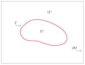
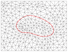
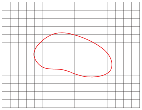
Figure 1: The simulation domain $\Omega$ (left), body-fitting mesh (middle), and non-body-fitting mesh (right).

Interface problems appear in many applications of engineering and science; therefore, it is of great importance to solve interface problems efficiently. When conventional finite element methods are employed to solve interface problems, body-fitting meshes (see the mid plot in Figure 1) have to be used in order to guarantee their optimal convergence [1, 2, 3, 5]. Such a restriction hinders their applications in some situations because it prevents the use of Cartesian mesh unless the interface has a very simple geometry such as an axis-parallel straight line. Recently, immersed finite element (IFE) methods have been developed to overcome such a limitation of traditional finite element methods for solving interface problems, see [6, 7, 8, 9, 12, 13, 14, 15, 18, 20, 23]. The main feature of IFE methods is that they can use interface independent meshes; hence, structured or even Cartesian meshes can be used to solve problems with nontrivial interface geometry (see the right plot in Figure 1). Most of IFE methods are developed for stationary interface problems. There are a few literatures of IFEs on time-dependent interface problems. For instance, an immersed Eulerian-Lagrangian localized adjoint method was developed to treat transient advection-diffusion equations with interfaces in [22]. In [19], IFE methods were applied to parabolic interface problem together with the Laplacian transform. Parabolic problems with moving interfaces were considered in [10, 16, 17] where Crank-Nicolson-type fully discrete IFE methods and IFE method of lines were derived through the Galerkin formulation.

For elliptic interface problems, classic IFE methods in Galerkin formulation [13, 14, 15] can usually converge to the exact solution with optimal order in $H^{1}$ and $L^{2}$ norm. Recently, the authors in [18, 23] observed that their orders of convergence in both $H^{1}$ and $L^{2}$ norms can sometimes deteriorate when the mesh size becomes very small, and this order degeneration might be the consequence of the discontinuity of IFE functions across interface edges (edges intersected with the interface). Note that IFE functions in [13, 14, 15] are constructed so that they are continuous within each interface element. On the boundary of an interface element, the continuity of these IFE functions is only imposed on two endpoints of each edge. This guarantees the continuity of IFE functions on non-interface edges. However, an IFE function is a piecewise polynomial on each interface edge; hence it is usually discontinuous on interface edges. This discontinuity depends on the interface location and the jump of coefficients, and could be large for certain configuration of interface element and diffusion coefficient. When the mesh is refined, the number of interface elements becomes larger, and such discontinuity over interface edges might be a factor negatively impacting on the global convergence.

To overcome the order degeneration of convergence, a partially penalized immersed finite element (PPIFE) formulation was introduced in [18, 23]. In the new formulation, additional stabilization terms generated on interface edges are added to the finite element equations that can penalize the discontinuity of IFE functions across interface edges. Since the number of interface edges is much smaller than the total number of elements of a Cartesian mesh, the computational cost for generating those partial penalty terms is negligible. For elliptic interface problems, the PPIFE methods can effectively reduce errors around interfaces; hence, maintain the optimal convergence rates under mesh refinement without degeneration.

Our goal here is to develop PPIFE methods for the parabolic interface problem (1.1) - (1.5) and to derive the a priori error estimates for these methods. We present the semi-discrete method and two prototypical fully discrete methods, i.e., the backward Euler method and Crank-Nicolson method in Section 2. In Section 3, the a priori error estimates are derived for these methods which indicate the optimal convergence from the point of view of polynomials used in the involved IFE subspaces. Finally, numerical examples are provided in Section 4 to validate the theoretical estimates.

In the discussion below, we will use a few general assumptions and notations. First, from now on, we will tacitly assume that the interface problem has a homogeneous boundary condition, i.e., $g=0$ for the simplicity of presentation. The methods and related analysis can be easily extended to problems with a non-homogeneous boundary condition through a standard procedure. Second, we will adopt standard notations and norms of Sobolev spaces. For $r\geq 1$ , we define the following function spaces:

$$\tilde{H}^{r}(\Omega)=\{v:v|_{\Omega^{s}}\in H^{r}(\Omega^{s}),s=+\ \text{or}\ -\}$$

equipped with the norm

$$\|v\|^{2}_{\tilde{H}^{r}(\Omega)}=\|v\|^{2}_{H^{r}(\Omega^{-})}+\|v\|^{2}_{H^{r}(\Omega^{+})},~{}~{}~{}\forall v\in\tilde{H}^{r}(\Omega).$$

For a function $z(X,t)$ with space variable $X=(x,y)$ and time variable $t$, we consider it as a mapping from the time interval $[0,T]$ to a normed space $V$ equipped with the norm $\|\cdot\|_{V}$. In particular, for an integer $k\geq 1$, we define

$$L^{k}(0,T;V)=\left\{z:[0,T]\rightarrow V~{}~{}\text{measurable, such that}\int_{0}^{T}\|z(\cdot,t)\|_{V}^{k}dt<\infty\right\}$$

with

$$\|z\|_{L^{k}(0,T;V)}=\left(\int_{0}^{T}\|z(\cdot,t)\|_{V}^{k}dt\right)^{1/k}.$$

Also, for $V=\tilde{H}^{r}(\Omega)$, we will use the standard function space $H^{p}(0,T;\tilde{H}^{r}(\Omega))$ for $p\geq 0,r\geq 1$.

In addition, we will use $C$ with or without subscript to denote a generic positive constant which may have different values according to its occurrence. For simplicity, we will use $u_{t}$, $u_{tt}$, etc., to denote the partial derivatives of a function $u$ with respect to the time variable $t$.

2 Partially Penalized Immersed Finite Element Methods

In this section, we first derive a weak formulation of the parabolic interface problem (1.1) - (1.5) based on Cartesian meshes. Then we recall bilinear IFE functions and spaces defined on rectangular meshes from [8, 15]. The construction of linear IFE functions on triangular meshes is similar, so we refer to [13, 14] for more details. Finally, we introduce the partially penalized immersed finite element methods for the parabolic interface problem.

2.1 Weak Form on Continuous Level

Let $\mathcal{T}_{h}$ be a Cartesian (either triangular or rectangular) mesh consisting of elements whose diameters are not larger than $h$. We denote by $\mathcal{N}_{h}$ and $\mathcal{E}_{h}$ the set of all vertices and edges in $\mathcal{T}_{h}$, respectively. The set of all interior edges are denoted by $\mathcal{\mathring{E}}_{h}$. If an element is cut by the interface $\Gamma$, we call it an interface element; otherwise, it is called a non-interface element. Let $\mathcal{T}_{h}^{i}$ be the set of interface elements and $\mathcal{T}_{h}^{n}$ be the set of non-interface elements. Similarly, we define the set of interface edges and the set of non-interface edges which are denoted by $\mathcal{E}_{h}^{i}$ and $\mathcal{E}_{h}^{n}$, respectively. Also, we use $\mathcal{\mathring{E}}_{h}^{i}$ and $\mathcal{\mathring{E}}_{h}^{n}$ to denote the set of interior interface edges and interior non-interface edges, respectively. With the assumption that $\Gamma\subset\Omega$ we have $\mathcal{\mathring{E}}_{h}^{i}=\mathcal{E}_{h}^{i}$.

We assign a unit normal vector $\mathbf{n}_{B}$ to every edge $B\in{{\mathcal{E}}}_{h}$. If $B$ is an interior edge, we let $K_{B,1}$ and $K_{B,2}$ be the two elements that share the common edge $B$ and we assume that the normal vector $\mathbf{n}_{B}$ is oriented from $K_{B,1}$ to $K_{B,2}$. For a function $u$ defined on $K_{B,1}\cup K_{B,2}$, we set its average and jump on $B$ as follows

$$\left\{\!\!\left\{u\right\}\!\!\right\}_{B}=\frac{1}{2}\left((u|_{K_{B,1}})|_{B}+(u|_{K_{B,2}})|_{B}\right),~{}~{}~{}~{}\left[\!\left[u\right]\!\right]_{B}=(u|_{K_{B,1}})|_{B}-(u|_{K_{B,2}})|_{B}.$$

If $B$ is on the boundary $\partial\Omega$, $\mathbf{n}_{B}$ is taken to be the unit outward vector normal to $\partial\Omega$, and we let

$$\left\{\!\!\left\{u\right\}\!\!\right\}_{B}=\left[\!\left[u\right]\!\right]_{B}=u|_{B}.$$

For simplicity, we often drop the subscript $B$ from these notations if there is no danger to cause any confusions.

Without loss of generality, we assume that the interface $\Gamma$ intersects with the edge of each interface element $K\in\mathcal{T}_{h}^{i}$ at two points. We then partition $K$ into two sub-elements $K^{-}$ and $K^{+}$ by the line segment connecting these two interface points, see the illustration given in Figure 2.

To describe a weak form for the parabolic interface problem, we introduce the following space

$$V_{h}=\{v\in L^{2}(\Omega):v\text{ satisfies conditions}\textbf{ (HV1) - (HV4)}\}$$ (2.1)

(HV1)

$v|_{K}\in H^{1}(K),v|_{K^{s}}\in H^{2}(K^{s}),s=\pm,\forall K\in\mathcal{T}_{h}$.

(HV2)

$v$ is continuous at every $X\in\mathcal{N}_{h}$.

(HV3)

$v$ is continuous across each $B\in{\mathring{\mathcal{E}}}_{h}^{n}$.

(HV4)

$v|_{\partial\Omega}=0$.

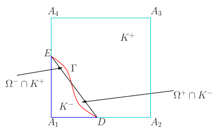
Figure 2: An interface element

Note that functions in $V_{h}$ are allowed to be discontinuous on interface edges. We now derive a weak form with the space $V_{h}$ for the parabolic interface problem (1.1) - (1.5). First, we assume that its exact solution $u$ is in $\tilde{H}^{2}(\Omega)$. Then, we multiply equation (1.1) by a test function $v\in V_{h}$ and integrate both sides on each element $K\in\mathcal{T}_{h}$. If $K$ is a non-interface element, a direct application of Green’s formula leads to

$$\int_{K}u_{t}vdX+\int_{K}\beta\nabla u\cdot\nabla vdX-\int_{\partial K}\beta\nabla u\cdot{\mathbf{n}_{K}}vds=\int_{K}fvdX.$$ (2.2)

If $K$ is an interface element, we assume that the interface $\Gamma$ intersects $\partial K$ at points $D$ and $E$. Then, without loss of generality, we assume that $\Gamma$ and the line $\overline{DE}$ divide $K$ into up to four sub-elements, see the illustration in Figure 2 for a rectangle interface element, such that

$$K=(\Omega^{+}\cap K^{+})\cup(\Omega^{-}\cap K^{-})\cup(\Omega^{+}\cap K^{-})\cup(\Omega^{-}\cap K^{+}).$$

Now, applying Green’s formula separately on these four sub-elements, we get

$$-\int_{K}\nabla\cdot(\beta\nabla u)vdX$$ (2.3)

$$= -\int_{\Omega^{+}\cap K^{+}}\nabla\cdot(\beta^{+}\nabla u)vdX-\int_{\Omega^{-}\cap K^{-}}\nabla\cdot(\beta^{-}\nabla u)vdX$$

$$-\int_{\Omega^{+}\cap K^{-}}\nabla\cdot(\beta^{+}\nabla u)vdX-\int_{\Omega^{-}\cap K^{+}}\nabla\cdot(\beta^{-}\nabla u)vdX$$

$$= \int_{\Omega^{+}\cap K^{+}}\beta^{+}\nabla u\cdot\nabla vdX-\int_{\partial(\Omega^{+}\cap K^{+})}\beta^{+}\nabla u\cdot{\mathbf{n}}vds+\int_{\Omega^{-}\cap K^{-}}\beta^{-}\nabla u\cdot\nabla vdX-\int_{\partial(\Omega^{-}\cap K^{-})}\beta^{-}\nabla u\cdot{\mathbf{n}}vds$$

$$+\int_{\Omega^{+}\cap K^{-}}\beta^{+}\nabla u\cdot\nabla vdX-\int_{\partial(\Omega^{+}\cap K^{-})}\beta^{+}\nabla u\cdot{\mathbf{n}}vds+\int_{\Omega^{-}\cap K^{+}}\beta^{-}\nabla u\cdot\nabla vdX-\int_{\partial(\Omega^{-}\cap K^{+})}\beta^{-}\nabla u\cdot{\mathbf{n}}vds$$

$$= \int_{K}\beta\nabla u\cdot\nabla vdX-\int_{\partial K}\beta\nabla u\cdot{\mathbf{n}}vds-\int_{K\cap\Gamma}\left[\!\left[\beta\nabla u\cdot{\mathbf{n}}\right]\!\right]_{K\cap\Gamma}vds$$

$$= \int_{K}\beta\nabla u\cdot\nabla vdX-\int_{\partial K}\beta\nabla u\cdot{\mathbf{n}}vds.$$

The last equality is due to the interface jump condition (1.5). The derivation of (2.3) implies that (2.2) also holds on interface elements.

Remark 2.1.

Figure 2 is a typical configuration of an interface element. If the interface is smooth enough and the mesh size is sufficiently small, an interface is usually divided into three sub-elements, i.e., one of the two terms $\Omega^{+}\cap K^{-}$ and $\Omega^{-}\cap K^{+}$ is an empty set. In this case, the related discussion is similar but slightly simpler.

Summarizing (2.2) over all elements indicates

$$\int_{\Omega}u_{t}vdX+\sum\limits_{K\in\mathcal{T}_{h}}\int_{K}\beta\nabla u\cdot\nabla vdX-\sum\limits_{B\in\mathring{\mathcal{E}}_{h}^{i}}\int_{B}\left\{\!\!\left\{\beta\nabla u\cdot\mathbf{n}_{B}\right\}\!\!\right\}\left[\!\left[v\right]\!\right]ds=\int_{\Omega}fvdX.$$ (2.4)

Let $H_{h}=\tilde{H}^{2}(\Omega)+V_{h}$ on which we introduce a bilinear form $a_{\epsilon}$: $H_{h}\times H_{h}\rightarrow\mathbb{R}$:

$$a_{\epsilon}(w,v) = \sum\limits_{K\in\mathcal{T}_{h}}\int_{K}\beta\nabla v\cdot\nabla wdX-\sum\limits_{B\in\mathring{\mathcal{E}}_{h}^{i}}\int_{B}\left\{\!\!\left\{\beta\nabla w\cdot\mathbf{n}_{B}\right\}\!\!\right\}\left[\!\left[v\right]\!\right]ds$$ (2.5)

$$+\epsilon\sum\limits_{B\in\mathring{\mathcal{E}}_{h}^{i}}\int_{B}\left\{\!\!\left\{\beta\nabla v\cdot\mathbf{n}_{B}\right\}\!\!\right\}\left[\!\left[w\right]\!\right]ds+\sum\limits_{B\in\mathring{\mathcal{E}}_{h}^{i}}\int_{B}\frac{\sigma^{0}_{B}}{|B|^{\alpha}}\left[\!\left[v\right]\!\right]\left[\!\left[w\right]\!\right]ds,$$

where $\alpha>0$, $\sigma^{0}_{B}\geq 0$ and $|B|$ means the length of $B$. Note that the regularity of $u$ leads to

$$\epsilon\sum\limits_{B\in\mathcal{\mathring{E}}_{h}^{i}}\int_{B}\left\{\!\!\left\{\beta\nabla v\cdot\mathbf{n}_{B}\right\}\!\!\right\}\left[\!\left[u\right]\!\right]ds=0,\ \ \sum\limits_{B\in\mathcal{\mathring{E}}_{h}^{i}}\int_{B}\frac{\sigma^{0}_{B}}{|B|^{\alpha}}\left[\!\left[v\right]\!\right]\left[\!\left[u\right]\!\right]ds=0.$$

We also define the following linear form

$$L(v)=\int_{\Omega}fvdX.$$

Finally, we have the following weak form of the parabolic interface problem (1.1)-(1.5): find $u:[0,T]\rightarrow\tilde{H}^{2}(\Omega)$ that satisfies (1.4), (1.5), and

$$\left(u_{t},v\right)+a_{\epsilon}(u,v) = L(v),\ \ \forall v\in V_{h},$$ (2.6)

$$u(X,0) = u_{0}(X),\ \ \forall X\in\Omega.$$ (2.7)

2.2 Immersed Finite Element Functions

In this subsection, to be self-contained, we recall IFE spaces that approximate $V_{h}$. We describe the bilinear IFE space with a little more details, and refer readers to [13, 14] for corresponding descriptions of the linear IFE space on a triangular Cartesian mesh. Since an IFE space uses standard finite element functions on each non-interface element, we will focus on the presentation of IFE functions on interface elements.

The bilinear ($Q_{1}$) immersed finite element functions were introduced in [8, 15]. On each interface element, a local IFE space uses IFE functions in the form of piecewise bilinear polynomials constructed according to interface jump conditions. Specifically, we partition each interface element $K=\square A_{1}A_{2}A_{3}A_{4}$ into two sub-elements $K^{-}$ and $K^{+}$ by the line connecting points $D$ and $E$ where the interface $\Gamma$ intersects with $\partial K$, see Figure 3 for illustrations. Then we construct four bilinear IFE shape functions $\phi_{i},i=1,2,3,4$ associated with the vertices of $K$ such that

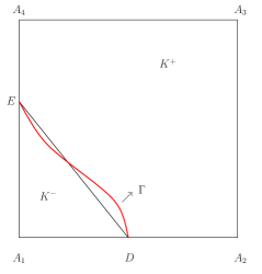
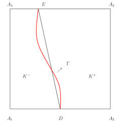
Figure 3: Type I and Type II interface rectangles

$$\phi_{i}(x,y)=\left\{\begin{array}[]{cc}\phi_{i}^{+}(x,y)=a_{i}^{+}+b_{i}^{+}x+c_{i}^{+}y+d_{i}^{+}xy,{}{}{}{}&\text{if}~{}(x,y)\in K^{+},\vspace{1mm}\\ \phi_{i}^{-}(x,y)=a_{i}^{-}+b_{i}^{-}x+c_{i}^{-}y+d_{i}^{-}xy,{}{}{}{}&\text{if}~{}(x,y)\in K^{-},\vspace{1mm}\\ \end{array}\right.$$ (2.8)

according to the following constraints:

• nodal value condition:

  $$\phi_{i}(A_{j})=\delta_{ij},~{}~{}~{}~{}~{}i,j=1,2,3,4.$$ (2.9)

• continuity on $\overline{DE}$

  $$\left[\!\left[\phi_{i}{(D)}\right]\!\right]=0,~{}~{}~{}~{}\left[\!\left[\phi_{i}{(E)}\right]\!\right]=0,~{}~{}~{}~{}\left[\!\!\left[\frac{\partial^{2}\phi_{i}}{\partial x\partial y}\right]\!\!\right]=0.$$ (2.10)

• continuity of normal component of flux

  $$\int_{\overline{DE}}\left[\!\!\left[\beta\frac{\partial\phi_{i}}{\partial n}\right]\!\!\right]\mbox{d}s=0.$$ (2.11)

It has been shown [7, 8] that conditions specified in (2.9) - (2.11) can uniquely determine these shape functions. Figure 4 provides a comparison of FE and IFE shape functions.

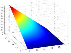
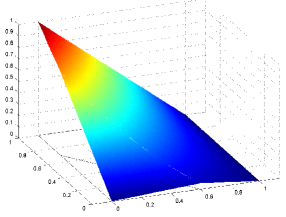
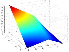
Figure 4: Bilinear FE/IFE local basis functions. From left: FE, IFE (Type I), IFE (Type II)

Similarly, see more details in [13, 14], on a triangular interface element $K=\triangle A_{1}A_{2}A_{3}$, we can construct three linear IFE shape functions $\phi_{i},i=1,2,3$ that satisfy the first two equations in (2.10), (2.11), and

$$\phi_{i}(A_{j})=\delta_{ij},~{}~{}~{}~{}~{}i,j=1,2,3.$$

These IFE shape functions possess a few notable properties such as their consistence with the corresponding standard Lagrange type FE shape functions and their formation of partition of unity. We refer readers to [7, 8, 13, 23] for more details.

Then, on each element $K\in\mathcal{T}_{h}$, we define the local IFE space as follows:

$$S_{h}(K)=span\{\phi_{i},~{}~{}1\leq i\leq d_{K}\},~{}~{}d_{K}=\begin{cases}3,&\text{if $K$ is a triangular element},\\ 4,&\text{if $K$ is a rectangular element},\end{cases}$$

where $\phi_{i},1\leq i\leq d_{K}$ are the standard linear or bilinear Lagrange type FE shape functions for $K\in\mathcal{T}_{h}^{n}$; otherwise, they are the IFE shape functions described above. Finally, the IFE spaces on the whole solution domain $\Omega$ are defined as follows:

$$S_{h}(\Omega) = \{v\in V_{h}~{}:~{}v|_{K}\in S_{h}(K),~{}\forall K\in\mathcal{T}_{h}\}.$$

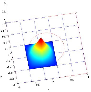
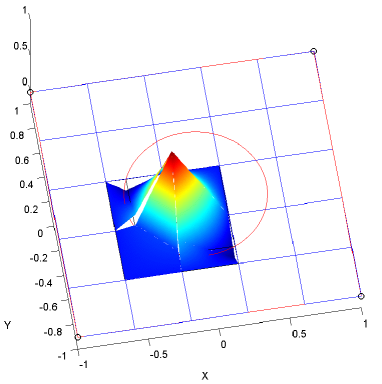
Figure 5: Bilinear FE (left) and IFE (right) global basis functions

Remark 2.2.

We note that an IFE function may not be continuous across the element boundary that intersects with the interface. An IFE shape function is usually not zero on an interface edge, see the values on the edge between the points $(0,0)$ and $(0,1)$ for the two IFE shape functions plotted in Figure 4. On this interface edge, the shape functions vanish at two endpoints, but not on the entire edge. The maximum of the absolute values of the shape on that edge is determined by the geometrical and material configuration on an interface element. When the local IFE shape functions are put together to form a Lagrange type global IFE basis function associated with a node in a mesh, it is inevitably to be discontinuous on interface edges in elements around that node, as illustrated by the cracks in a global IFE basis function plotted in Figure 5. As observed in [18, 23], this discontinuity on interface edges might be a factor causing the deterioration of the convergence of classic IFE solution around the interface, and this motivates us to add partial penalty on interface edges for alleviating this adversary.

2.3 Partially Penalized Immersed Finite Element Methods

In this subsection we use the global IFE space $S_{h}(\Omega)$ to discretize the weak form (2.6) and (2.7) for the parabolic interface problem. While the standard semi-discrete or many fully discrete frameworks can be applied, we will focus on the following prototypical schemes because of their popularity.

A semi-discrete PPIFE method: Find $u_{h}:[0,T]\rightarrow S_{h}(\Omega)$ such that

$$\left(u_{h,t},v_{h}\right)+a_{\epsilon}(u_{h},v_{h}) = L(v_{h}),\ \ \forall v_{h}\in S_{h}(\Omega),$$ (2.12)

$$u_{h}(X,0) = \tilde{u}_{h}(X),\ \ \forall X\in\Omega,$$ (2.13)

where $\tilde{u}_{h}$ is an approximation of $u_{0}$ in the space $S_{h}(\Omega)$. According to the analysis to be carried out in the next section, $\tilde{u}_{h}$ can be chosen as the interpolation of $u_{0}$ or the elliptic projection of $u_{0}$ in the IFE space $S_{h}(\Omega)$.

A fully discrete PPIFE method: For a positive integer $N_{t}$, we let $\Delta t=T/N_{t}$ which is the time step and let $t^{n}=n\Delta t$ for integer $n\geq 0$. Also, for a sequence $\varphi^{n},n\geq 1$, we let

$$\partial_{t}\varphi^{n}=\frac{\varphi^{n}-\varphi^{n-1}}{\Delta t}.$$

Then, the fully discrete PPIFE method is to find a sequence $\big{\{}u_{h}^{n}\big{\}}_{n=1}^{N_{t}}$ of functions in $S_{h}(\Omega)$ such that

$$\left(\partial_{t}u_{h}^{n},v_{h}\right)+a_{\epsilon}(\theta u_{h}^{n}+(1-\theta)u_{h}^{n-1},v_{h}) = \theta L^{n}(v_{h})+(1-\theta)L^{n-1}(v_{h}),~{}~{}\forall v_{h}\in S_{h}(\Omega),$$ (2.14)

$$u_{h}^{0}(X) = \tilde{u}_{h}(X),\ \ \forall X\in\Omega.$$ (2.15)

Here, $L^{n}(v_{h})=\int_{\Omega}f(X,t^{n})v_{h}(X)dX,n\geq 0$ and $\theta$ is a parameter chosen from $[0,1]$. Popular choices for $\theta$ are $\theta=0,\theta=1$ and $\theta=1/2$ representing the forward Euler method, the backward Euler method, and the Crank-Nicolson method, respectively.

Remark 2.3.

The bilinear form $a_{\epsilon}(\cdot,\cdot)$ in (2.6) is almost the same as that used in the interior penalty DG finite element methods for the standard elliptic boundary value problem [4, 11, 21] except that it contains integrals over interface edges instead of all the edges. This is why we call IFE methods based on this bilinear form partially penalized IFE (PPIFE) methods. As suggested by DG finite element methods, the parameter $\epsilon$ in this bilinear form is usually chosen as $-1$, $0$, or $1$. Note that $a_{\epsilon}(\cdot,\cdot)$ is symmetric if $\epsilon=-1$ and is nonsymmetric otherwise.

3 Error Estimations for PPIFE Methods

The goal of this section is to derive the a priori error estimates for the PPIFE methods developed in the previous section. As usual, without loss of generality for error estimation, we assume that $g(X,t)=0$ in the boundary condition (1.2) and assume $\Gamma\cap\partial\Omega=\emptyset$. The error bounds will be given in an energy norm that is equivalent to the standard semi-$H^{1}$ norm. These error bounds show that these PPIFE methods converge optimally with respect to the polynomials employed.

3.1 Some Preliminary Estimates

First, for every $v\in V_{h}$, we define its energy norm as follows:

$$\|v\|_{h}=\left(\sum\limits_{K\in\mathcal{T}_{h}}\int_{K}\beta\nabla v\cdot\nabla vdX+\sum\limits_{B\in\mathring{\mathcal{E}}_{h}^{i}}\int_{B}\frac{\sigma_{B}^{0}}{|B|^{\alpha}}\left[\!\left[v\right]\!\right]\left[\!\left[v\right]\!\right]ds\right)^{1/2}.$$

For an element $K\in\mathcal{T}_{h}$, let $|K|$ denote the area of $K$. It is well known that the following trace inequalities [21] hold:

Lemma 3.1.

There exists a constant $C$ independent of $h$ such that for every $K\in\mathcal{T}_{h}$,

$$\|v\|_{L^{2}(B)}\leq C|B|^{1/2}|K|^{-1/2}(\|v\|_{L^{2}(K)}+h\|\nabla v\|_{L^{2}(K)}),\ \forall v\in H^{1}(K),~{}B\subset\partial K,$$ (3.1)

$$\|\nabla v\|_{L^{2}(B)}\leq C|B|^{1/2}|K|^{-1/2}(\|\nabla v\|_{L^{2}(K)}+h\|\nabla^{2}v\|_{L^{2}(K)}),\ \forall v\in H^{2}(K),~{}B\subset\partial K.$$ (3.2)

Since the local IFE space $S_{h}(K)\subset H^{1}(K)$ for all $K\in\mathcal{T}_{h}$ (e.g. [7, 8, 13]), the trace inequality (3.1) is valid for all $v\in S_{h}(K)$. However, for $K\in\mathcal{T}_{h}^{i}$, a function $v\in S_{h}(K)$ does not belong to $H^{2}(K)$ in general. So the second trace inequality (3.2) cannot be directly applied to IFE functions. Nevertheless, for linear and bilinear IFE functions, the corresponding trace inequalities have been established in [18]. The related results are summarized in the following lemma.

Lemma 3.2.

There exists a constant $C$ independent of interface location and $h$ but depending on the ratio of coefficients $\beta^{+}$ and $\beta^{-}$ such that for every linear or bilinear IFE function $v$ on $K\in\mathcal{T}_{h}^{i}$,

$$\|\beta v_{d}\|_{L^{2}(B)}\leq Ch^{1/2}|K|^{-1/2}\|\sqrt{\beta}\nabla v\|_{L^{2}(K)},\ \forall v\in S_{h}(K),B\subset\partial K,d=x\ \text{or}\ y,$$ (3.3)

$$\|\beta\nabla v\cdot\mathbf{n}_{B}\|_{L^{2}(B)}\leq Ch^{1/2}|K|^{-1/2}\|\sqrt{\beta}\nabla v\|_{L^{2}(K)},\ \ \forall v\in S_{h}(K),B\subset\partial K.$$ (3.4)

As in [18], using Young’s inequality, trace inequalities and the definition of $\|\cdot\|_{h}$, we can prove the coercivity of the bilinear form $a_{\epsilon}(\cdot,\cdot)$ on the IFE space $S_{h}(\Omega)$ with respect to the energy norm $\|\cdot\|_{h}$. The result is stated in the lemma below.

Lemma 3.3.

There exists a constant $\kappa>0$ such that

$$a_{\epsilon}(v_{h},v_{h})\geq\kappa\|v_{h}\|_{h}^{2},\ \ \forall v_{h}\in S_{h}(\Omega)$$ (3.5)

holds for $\epsilon=1$ unconditionally and holds for $\epsilon=0$ or $\epsilon=-1$ when the penalty parameter $\sigma_{B}^{0}$ in $a_{\epsilon}(\cdot,\cdot)$ is large enough and $\alpha\geq 1$.

For any $t\in[0,T]$, we define the elliptic projection of the exact solution $u(\cdot,t)$ as the IFE function $\tilde{u}_{h}(\cdot,t)\in S_{h}(\Omega)$ by

$$a_{\epsilon}(u-\tilde{u}_{h},v_{h})=0,\ \ \forall v_{h}\in S_{h}(\Omega).$$ (3.6)

Lemma 3.4.

Assume the exact solution $u$ is in $H^{2}(0,T;\tilde{H}^{3}(\Omega))$ and $\alpha=1$. Then there exists a constant $C$ such that for every $t\in[0,T]$ the following error estimates hold

$$\|u-\tilde{u}_{h}\|_{h}\leq Ch\|u\|_{\tilde{H}^{3}(\Omega)},$$ (3.7)

$$\|(u-\tilde{u}_{h})_{t}\|_{h}\leq Ch\|u_{t}\|_{\tilde{H}^{3}(\Omega)}.$$ (3.8)

$$\|(u-\tilde{u}_{h})_{tt}\|_{h}\leq Ch\|u_{tt}\|_{\tilde{H}^{3}(\Omega)}.$$ (3.9)

Proof.

First, the estimate (3.7) follows directly from the estimate derived for the PPIFE methods for elliptic problems in [18]. Because of the linearity of the bilinear form, we have that

$$a_{\epsilon}\left((u-\tilde{u}_{h})_{t},v_{h}\right)=\frac{d}{dt}a_{\epsilon}(u-\tilde{u}_{h},v_{h})=0,\ \ \forall v_{h}\in S_{h}(\Omega).$$

This indicates that the time derivative of the elliptic projection is the elliptic projection of the time derivative. Thus, for any given $t\in[0,T]$, $u_{t}\in\tilde{H}^{3}(\Omega)$, the estimate (3.8) follows from the estimate derived for the PPIFE methods for elliptic problems in [18] again. Similarly, we can obtain (3.9). ∎

3.2 Error estimation for the semi-discrete method

The a priori error estimates for semi-discrete PPIFE method (2.12)-(2.13) for parabolic interface problem is given in the following theorem.

Theorem 3.1.

Assume that the exact solution $u$ to the parabolic interface problem (1.1)-(1.5) is in $H^{1}(0,T;\tilde{H}^{3}(\Omega))$ for $\epsilon=-1$ and in $H^{2}(0,T;\tilde{H}^{3}(\Omega))$ when $\epsilon=0,1$, and $u_{0}\in\tilde{H}^{3}(\Omega)$. Let $u_{h}$ be the PPIFE solution defined by semi-discrete method (2.12)-(2.13) with $\alpha=1$ and $u_{h}(\cdot,0)=\tilde{u}_{h}(\cdot)$ being the elliptic projection of $u_{0}$. Then there exists a constant $C$ such that

$$\|u(\cdot,t)-u_{h}(\cdot,t)\|_{h}\leq Ch\Big{(}\|u_{0}\|_{\tilde{H}^{3}(\Omega)}+\|u_{t}\|_{L^{2}(0,T;\tilde{H}^{3}(\Omega))}\Big{)},\ \ \forall t\geq 0,$$ (3.10)

for $\epsilon=-1$, and

$$\|u(\cdot,t)-u_{h}(\cdot,t)\|_{h}$$

$$\leq Ch\Big{(}\|u_{0}\|_{\tilde{H}^{3}(\Omega)}+\|u_{t}(\cdot,0)\|_{\tilde{H}^{3}(\Omega)}+\|u_{t}\|_{L^{2}(0,T;\tilde{H}^{3}(\Omega))}+\|u_{tt}\|_{L^{2}(0,T;\tilde{H}^{3}(\Omega))}\Big{)},\ \ \forall t\geq 0,$$ (3.11)

for $\epsilon=0$ or 1.

Proof.

Let $\tilde{u}_{h}$ be the elliptic projection of $u$ defined by (3.6) and we use it to split the error $u-u_{h}$ into two terms: $u-u_{h}=\eta-\xi$ with $\eta=u-\tilde{u}_{h}$ and $\xi=u_{h}-\tilde{u}_{h}$. For the first term, by (3.7), we have the following estimate:

$$\|\eta(\cdot,t)\|_{h} \leq Ch\|u(\cdot,t)\|_{\tilde{H}^{3}(\Omega)}\leq Ch\Big{(}\|u_{0}\|_{\tilde{H}^{3}(\Omega)}+\int_{0}^{t}\|u_{t}\|_{\tilde{H}^{3}(\Omega)}d\tau\Big{)}$$ (3.12)

$$\leq Ch\Big{(}\|u_{0}\|_{\tilde{H}^{3}(\Omega)}+\|u_{t}\|_{L^{2}(0,T;\tilde{H}^{3}(\Omega))}\Big{)}.$$

Then, we proceed to bound $\|\xi\|_{h}$. From (2.6), (2.12) and (3.6), we can see that $\xi$ satisfies the following equation:

$$\left(\xi_{t},v_{h}\right)+a_{\epsilon}(\xi,v_{h})=\left(\eta_{t},v_{h}\right),\ \ \forall v_{h}\in S_{h}(\Omega).$$ (3.13)

Choosing $v_{h}=\xi_{t}$ in (3.13), we have

$$\|\xi_{t}\|^{2}+a_{\epsilon}(\xi,\xi_{t})=\left(\eta_{t},\xi_{t}\right).$$ (3.14)

If $\epsilon=-1$, using the symmetry property of $a_{\epsilon}(\cdot,\cdot)$, Cauchy-Schwarz inequality and Young’s inequality in (3.14), we get

$$\left\|\xi_{t}\right\|^{2}+\frac{1}{2}\frac{d}{dt}a_{\epsilon}(\xi,\xi)\leq\|\eta_{t}\|\left\|\xi_{t}\right\|\leq C\left\|\eta_{t}\right\|^{2}+\frac{1}{2}\left\|\xi_{t}\right\|^{2}.$$ (3.15)

For any $t\in(0,T]$, integrating both sides of (3.15) from 0 to $t$, using the fact $\xi(\cdot,0)=0$ and (3.8), we obtain

$$\frac{1}{2}\int_{0}^{t}\left\|\xi_{t}\right\|^{2}+\frac{1}{2}a_{\epsilon}(\xi(\cdot,t),\xi(\cdot,t))\leq C\int_{0}^{t}\left\|\eta_{t}\right\|^{2}dt\leq Ch^{2}\int_{0}^{T}\left\|u_{t}\right\|_{\tilde{H}^{3}(\Omega)}^{2}.$$ (3.16)

Using coercivity of $a_{\epsilon}(\cdot,\cdot)$ in (3.16), we have

$$\|\xi_{t}\|_{L^{2}(0,t;L^{2}(\Omega))}+\|\xi\|_{h}\leq Ch\|u_{t}\|_{L^{2}(0,T;\tilde{H}^{3}(\Omega))}.$$ (3.17)

Finally, applying the triangle inequality, (3.12) and (3.17) to $u-u_{h}=\eta-\xi$ leads to (3.10).

When $\epsilon=1$ or $0$, $a_{\epsilon}(\cdot,\cdot)$ is not symmetric. However, we have

$$a_{\epsilon}\left(\xi,\xi_{t}\right) = \frac{1}{2}\frac{d}{dt}a_{\epsilon}(\xi,\xi)+\frac{1}{2}\left(a_{\epsilon}\left(\xi,\xi_{t}\right)-a_{\epsilon}\left(\xi_{t},\xi\right)\right)$$ (3.18)

$$\geq \frac{1}{2}\frac{d}{dt}a_{\epsilon}(\xi,\xi)-C\|\xi_{t}\|_{h}\|\xi\|_{h}$$

$$\geq \frac{1}{2}\frac{d}{dt}a_{\epsilon}(\xi,\xi)-\frac{C}{2}\left\|\xi_{t}\right\|_{h}^{2}-\frac{C}{2}\|\xi\|_{h}^{2}.$$

Substituting (3.18) into (3.14) and then integrating it from 0 to $t$, we can get

$$\frac{1}{2}\int_{0}^{t}\|\xi_{t}\|^{2}d\tau+\frac{1}{2}\kappa\|\xi\|_{h}^{2}\leq C\int_{0}^{t}(\|\eta_{t}\|^{2}+\|\xi_{t}\|_{h}^{2}+\|\xi\|_{h}^{2})d\tau.$$ (3.19)

Now we need the bound of $\left\|\xi_{t}\right\|_{h}$. From (3.13), we can easily get

$$\left(\xi_{tt},v_{h}\right)+a_{\epsilon}(\xi_{t},v_{h})=\left(\eta_{tt},v_{h}\right),\ \ \forall v_{h}\in S_{h}(\Omega),t\geq 0.$$ (3.20)

Choose $v_{h}=\xi_{t}$ in (3.20) and use the coercivity of $a_{\epsilon}(\cdot,\cdot)$ to get

$$\frac{1}{2}\frac{d}{dt}\|\xi_{t}\|^{2}+\kappa\|\xi_{t}\|_{h}^{2}\leq\frac{1}{2}(\|\eta_{tt}\|^{2}+\|\xi_{t}\|^{2}).$$

Integrating the above inequality from 0 to $t$ and using the Gronwall inequality, we obtain

$$\int_{0}^{t}\|\xi_{t}\|_{h}^{2}d\tau\leq C\int_{0}^{t}\|\eta_{tt}\|^{2}d\tau+C\|\xi_{t}(\cdot,0)\|^{2}.$$ (3.21)

Let $t=0$ and then choose $v_{h}=\xi_{t}(\cdot,0)$ in (3.13) to get

$$\|\xi_{t}(\cdot,0)\|\leq\|\eta_{t}(\cdot,0)\|.$$ (3.22)

Substituting (3.21) and (3.22) into (3.19) and then using the Gronwall inequality again, we obtain

$$\int_{0}^{t}\|\xi_{t}\|^{2}d\tau+\|\xi\|_{h}^{2}\leq C\int_{0}^{t}(\|\eta_{t}\|^{2}+\|\eta_{tt}\|^{2})d\tau+C\|\eta_{t}(\cdot,0)\|^{2}.$$

Applying (3.8) and (3.9) to the above yields

$$\left\|\xi_{t}\right\|_{L^{2}(0,t;L^{2}(\Omega))}+\|\xi\|_{h}\leq Ch\Big{(}\|u_{t}(\cdot,0)\|_{\tilde{H}^{3}(\Omega))}+\|u_{t}\|_{L^{2}(0,T;\tilde{H}^{3}(\Omega))}+\|u_{tt}\|_{L^{2}(0,T;\tilde{H}^{3}(\Omega))}\Big{)}.$$ (3.23)

Finally, applying the triangle inequality, (3.12) and (3.23) to $u-u_{h}=\eta-\xi$ yields (3.11). ∎

Remark 3.1.

By slightly modifying the proof for Theorem 3.1 we can show that estimates (3.10) and (3.11) still hold when $\tilde{u}_{h}$ is chosen to be the IFE interpolation of $u_{0}$.

3.3 Error estimation for fully discrete methods

In all the discussion from now on, we assume that $u_{h}^{0}=\tilde{u}_{h}$ is the elliptic projection of $u_{0}$ in the initial condition for the parabolic interface problem. Also, for a function $\phi(t)$, we let $\phi^{n}=\phi(t^{n}),n\geq 0$.

3.3.1 Backward Euler method

The backward Euler method corresponds to the method described by (2.14) with $\theta=1$. From (2.6), (2.14) and (3.6), we get

$$\left(\partial_{t}\xi^{n},v_{h}\right)+a_{\epsilon}(\xi^{n},v_{h})=\left(\partial_{t}\eta^{n},v_{h}\right)+(r^{n},v_{h}),\ \ \forall v_{h}\in S_{h}(\Omega),$$ (3.24)

where $r^{n}=-(u_{t}^{n}-\partial_{t}u^{n})$. We choose the test function $v_{h}=\partial_{t}\xi^{n}$ in (3.24) and use the Cauchy-Schwarz inequality on the right hand side to obtain

$$\|\partial_{t}\xi^{n}\|^{2}+a_{\epsilon}(\xi^{n},\partial_{t}\xi^{n})\leq\Big{(}\|\partial_{t}\eta^{n}\|+\|r^{n}\|\Big{)}\|\partial_{t}\xi^{n}\|\leq\Big{(}\|\partial_{t}\eta^{n}\|^{2}+\|r^{n}\|^{2}\Big{)}+\frac{1}{2}\|\partial_{t}\xi^{n}\|^{2}.$$ (3.25)

There are three cases depending on the parameter $\epsilon$. We start from the case in which $\epsilon=-1$. By the symmetry and the coercivity of the bilinear form $a_{\epsilon}(\cdot,\cdot)$, we have

$$a_{\epsilon}(\xi^{n},\partial_{t}\xi^{n}) = \frac{1}{\Delta t}a_{\epsilon}(\xi^{n},\xi^{n}-\xi^{n-1})$$

$$= \frac{1}{2\Delta t}\Big{(}a_{\epsilon}(\xi^{n},\xi^{n})-a_{\epsilon}(\xi^{n-1},\xi^{n-1})\Big{)}+\frac{1}{2\Delta t}a_{\epsilon}(\xi^{n}-\xi^{n-1},\xi^{n}-\xi^{n-1})$$

$$\geq \frac{1}{2\Delta t}\Big{(}a_{\epsilon}(\xi^{n},\xi^{n})-a_{\epsilon}(\xi^{n-1},\xi^{n-1})\Big{)}.$$

Thus, we have

$$\frac{1}{2}\|\partial_{t}\xi^{n}\|^{2}+\frac{1}{2\Delta t}\Big{(}a_{\epsilon}(\xi^{n},\xi^{n})-a_{\epsilon}(\xi^{n-1},\xi^{n-1})\Big{)}\leq\|\partial_{t}\eta^{n}\|^{2}+\|r^{n}\|^{2}.$$ (3.26)

Multiply (3.26) by $2\Delta t$ and then sum over $n$ to get

$$\Delta t\sum\limits_{n=1}^{k}\|\partial_{t}\xi^{n}\|^{2}+a_{\epsilon}(\xi^{k},\xi^{k})\leq 2\Delta t\sum\limits_{n=1}^{k}\Big{(}\|\partial_{t}\eta^{n}\|^{2}+\|r^{n}\|^{2}\Big{)}.$$ (3.27)

By Hölder’s inequality and (3.8), we have

$$\|\partial_{t}\eta^{n}\|^{2} = \int_{\Omega}\left(\frac{\eta^{n}-\eta^{n-1}}{\Delta t}\right)^{2}dX=\int_{\Omega}\Big{(}\frac{1}{\Delta t}\int_{t^{n-1}}^{t^{n}}\eta_{t}d\tau\Big{)}^{2}dX$$ (3.28)

$$\leq \frac{1}{\Delta t}\int_{t^{n-1}}^{t^{n}}\|\eta_{t}\|^{2}d\tau\leq C\frac{h^{2}}{\Delta t}\int_{t^{n-1}}^{t^{n}}\|u_{t}\|_{\tilde{H}^{3}(\Omega)}^{2}d\tau.$$

Applying Taylor formula and Hölder’s inequality, we have

$$\|r^{n}\|^{2}=\int_{\Omega}|u_{t}^{n}-\partial_{t}u^{n}|^{2}dX=\int_{\Omega}\left|\frac{1}{\Delta t}\int_{t^{n-1}}^{t^{n}}(t-t^{n-1})u_{tt}dt\right|^{2}dX\leq\frac{\Delta t}{3}\int_{t^{n-1}}^{t^{n}}\|u_{tt}\|^{2}d\tau.$$ (3.29)

Substituting (3.28) and (3.29) into (3.27) and then using the coercivity of $a_{\epsilon}(\cdot,\cdot)$, we obtain

$$\Delta t\sum\limits_{n=1}^{k}\|\partial_{t}\xi^{n}\|^{2}+\|\xi^{k}\|_{h}^{2}\leq C\Big{(}h^{2}\|u_{t}\|_{L^{2}(0,T;\tilde{H}^{3}(\Omega))}^{2}+(\Delta t)^{2}\|u_{tt}\|_{L^{2}(0,T;L^{2}(\Omega))}^{2}\Big{)}.$$ (3.30)

Finally, applying the triangle inequality, (3.13) and (3.30) to $u^{k}-u_{h}^{k}=\eta^{k}-\xi^{k}$ yields

$$\|u^{k}-u_{h}^{k}\|_{h}\leq C\Big{(}h\big{(}\|u_{0}\|_{\tilde{H}^{3}(\Omega)}+\|u_{t}\|_{L^{2}(0,T;\tilde{H}^{3}(\Omega))}\big{)}+\Delta t\|u_{tt}\|_{L^{2}(0,T;L^{2}(\Omega))}\Big{)}$$ (3.31)

for any integer $k\geq 0$.

Now we turn to the cases where $\epsilon=0$ or $\epsilon=1$ that make the bilinear form in the PPIFE methods nonsymmetric. We start from

$$a_{\epsilon}(\xi^{n},\partial_{t}\xi^{n}) = \frac{1}{\Delta t}a_{\epsilon}(\xi^{n},\xi^{n}-\xi^{n-1})$$

$$= \frac{1}{2\Delta t}\Big{(}a_{\epsilon}(\xi^{n},\xi^{n})-a_{\epsilon}(\xi^{n-1},\xi^{n-1})\Big{)}+\frac{1}{2\Delta t}a_{\epsilon}(\xi^{n},\xi^{n}-\xi^{n-1})-\frac{1}{2\Delta t}a_{\epsilon}(\xi^{n}-\xi^{n-1},\xi^{n-1})$$

$$= \frac{1}{2\Delta t}\Big{(}a_{\epsilon}(\xi^{n},\xi^{n})-a_{\epsilon}(\xi^{n-1},\xi^{n-1})\Big{)}+\frac{1}{2}\Big{(}a_{\epsilon}(\xi^{n},\partial_{t}\xi^{n})-a_{\epsilon}(\partial_{t}\xi^{n},\xi^{n-1})\Big{)}$$

$$\geq \frac{1}{2\Delta t}\Big{(}a_{\epsilon}(\xi^{n},\xi^{n})-a_{\epsilon}(\xi^{n-1},\xi^{n-1})\Big{)}-C\Big{(}\|\partial_{t}\xi^{n}\|_{h}^{2}+\|\xi^{n-1}\|_{h}^{2}+\|\xi^{n}\|_{h}^{2}\Big{)}.$$

Substituting it into (3.25) leads to

$$\frac{1}{2}\|\partial_{t}\xi^{n}\|^{2}+\frac{1}{2\Delta t}\Big{(}a_{\epsilon}(\xi^{n},\xi^{n})-a_{\epsilon}(\xi^{n-1},\xi^{n-1})\Big{)}$$

$$\qquad\leq\|\partial_{t}\eta^{n}\|^{2}+\|r^{n}\|^{2}+C\Big{(}\|\partial_{t}\xi^{n}\|_{h}^{2}+\|\xi^{n-1}\|_{h}^{2}+\|\xi^{n}\|_{h}^{2}\Big{)}.$$ (3.32)

Multiply (3.32) by $2\Delta t$ and sum over $n$ to obtain

$$\sum\limits_{n=1}^{k}\Delta t\|\partial_{t}\xi^{n}\|^{2}+\kappa\|\xi^{k}\|_{h}^{2}\leq\sum\limits_{n=1}^{k}\Delta t(\|\partial_{t}\eta^{n}\|^{2}+\|r^{n}\|^{2})+C\sum\limits_{n=1}^{k}\Delta t\|\partial_{t}\xi^{n}\|_{h}^{2}+C\sum\limits_{n=1}^{k}\Delta t\|\xi^{n}\|_{h}^{2}.$$ (3.33)

In order to bound $\sum\limits_{n=1}^{k}\Delta t\|\partial_{t}\xi^{n}\|_{h}^{2}$, we first derive from (3.24) that

$$\frac{1}{\Delta t}\left(\partial_{t}\xi^{n}-\partial_{t}\xi^{n-1},v_{h}\right)+a_{\epsilon}(\partial_{t}\xi^{n},v_{h})=\left(\partial_{tt}\eta^{n},v_{h}\right)+(\partial_{t}r^{n},v_{h}),\ \ \forall v_{h}\in S_{h}(\Omega).$$ (3.34)

Let $v_{h}=\partial_{t}\xi^{n}$ in (3.34) to get

$$\frac{1}{2\Delta t}\left(\|\partial_{t}\xi^{n}\|^{2}-\|\partial_{t}\xi^{n-1}\|^{2}\right)+\kappa\|\partial_{t}\xi^{n}\|_{h}^{2}\leq(\|\partial_{tt}\eta^{n}\|+\|\partial_{t}r^{n}\|)\|\partial_{t}\xi^{n}\|.$$

Then we can easily obtain

$$\|\partial_{t}\xi^{k}\|^{2}+\sum\limits_{n=2}^{k}\Delta t\|\partial_{t}\xi^{n}\|_{h}^{2}\leq C\sum\limits_{n=2}^{k}\Delta t(\|\partial_{tt}\eta^{n}\|^{2}+\|\partial_{t}r^{n}\|^{2})+C\|\partial_{t}\xi^{1}\|^{2}.$$ (3.35)

Let $n=1$ and $v_{h}=\partial_{t}\xi^{1}=\xi^{1}/\Delta t$ in (3.24), then we have

$$\|\partial_{t}\xi^{1}\|^{2}+\frac{1}{\Delta t}a_{\epsilon}(\xi^{1},\xi^{1})\leq(\|\partial_{t}\eta^{1}\|+\|r^{1}\|)\|\partial_{t}\xi^{1}\|.$$

Thus

$$\|\partial_{t}\xi^{1}\|^{2}+\frac{1}{\Delta t}\|\xi^{1}\|_{h}^{2}\leq C(\|\partial_{t}\eta^{1}\|^{2}+\|r^{1}\|^{2}).$$

Applying this to (3.35) yields

$$\sum\limits_{n=1}^{k}\Delta t\|\partial_{t}\xi^{n}\|_{h}^{2}\leq C\sum\limits_{n=2}^{k}\Delta t(\|\partial_{tt}\eta^{n}\|^{2}+\|\partial_{t}r^{n}\|^{2})+C(\|\partial_{t}\eta^{1}\|^{2}+\|r^{1}\|^{2}).$$ (3.36)

Inserting (3.36) into (3.33), then applying the Gronwall inequality, we obtain

$$\|\xi^{k}\|_{h}^{2}\leq C\sum\limits_{n=1}^{k}\Delta t(\|\partial_{t}\eta^{n}\|^{2}+\|r^{n}\|^{2})+C\sum\limits_{n=2}^{k}\Delta t(\|\partial_{tt}\eta^{n}\|^{2}+\|\partial_{t}r^{n}\|^{2})+C(\|\partial_{t}\eta^{1}\|^{2}+\|r^{1}\|^{2}).$$ (3.37)

We now estimate the last four terms in (3.37). It is easily to see that

$$\|\partial_{tt}\eta^{n}\|^{2} = \int_{\Omega}\left(\frac{\eta^{n}-2\eta^{n-1}+\eta^{n-2}}{(\Delta t)^{2}}\right)^{2}dX$$

$$= \int_{\Omega}\left(\frac{1}{(\Delta t)^{2}}\int_{t^{n-1}}^{t^{n}}\eta_{tt}(t^{n}-t)dt-\frac{1}{(\Delta t)^{2}}\int_{t^{n-2}}^{t^{n-1}}\eta_{tt}(t^{n-1}-t)dt\right)^{2}dX$$

$$\leq \frac{1}{3\Delta t}\int_{t^{n-2}}^{t^{n}}\|\eta_{tt}\|^{2}dt.$$

This inequality and (3.9) lead to

$$\sum\limits_{n=2}^{k}\Delta t\|\partial_{tt}\eta^{n}\|^{2}\leq Ch^{2}\|u_{tt}\|^{2}_{L^{2}(0,T;\tilde{H}^{3}(\Omega))}.$$ (3.38)

Also, we have

$$\partial_{t}r^{n} = \frac{u_{t}^{n}-u_{t}^{n-1}}{\Delta t}-\frac{u^{n}-2u^{n-1}+u^{n-2}}{(\Delta t)^{2}}$$

$$= \int_{t^{n-1}}^{t^{n}}u_{ttt}dt-\frac{1}{(\Delta t)^{2}}\int_{t^{n-1}}^{t^{n}}u_{ttt}(t^{n-1}-t)^{2}dt+\frac{1}{(\Delta t)^{2}}\int_{t^{n-2}}^{t^{n-1}}u_{ttt}(t-t^{n-2})^{2}dt.$$

Then, the application of Hölder’s inequality leads to

$$\sum\limits_{n=2}^{k}\Delta t\|\partial_{t}r^{n}\|^{2} \leq (\Delta t)^{2}\sum\limits_{n=2}^{k}\left(\int_{t^{n-1}}^{t^{n}}\|u_{ttt}\|^{2}dt+\frac{1}{5}\int_{t^{n-1}}^{t^{n}}\|u_{ttt}\|^{2}dt+\frac{1}{5}\int_{t^{n-2}}^{t^{n-1}}\|u_{ttt}\|^{2}dt\right)$$ (3.39)

$$\leq C(\Delta t)^{2}\|u_{ttt}\|^{2}_{L^{2}(0,T;L^{2}(\Omega))}.$$

As for the last two terms on the right hand side of (3.37), we have

$$\|\partial_{t}\eta^{1}\|^{2}\leq\frac{1}{\Delta t}\int_{0}^{\Delta t}\|\eta_{t}\|^{2}dt\leq h^{2}\left(\frac{1}{\Delta t}\int_{0}^{\Delta t}\|u_{t}\|_{\tilde{H}^{3}(\Omega)}^{2}dt\right)$$ (3.40)

and, by (3.29),

$$\|r^{1}\|^{2}=\int_{\Omega}|u_{t}^{1}-\partial_{t}u^{1}|^{2}dX\leq\frac{(\Delta t)^{2}}{3}\left(\frac{1}{\Delta t}\int_{0}^{\Delta t}\|u_{tt}\|^{2}dt\right).$$ (3.41)

Now, substituting (3.28), (3.29) and (3.38)-(3.41) into (3.37), we obtain

$$\|\xi^{k}\|_{h}^{2} \leq C\left(\|u_{t}\|_{L^{2}(0,T;\tilde{H}^{3}(\Omega))}^{2}+\|u_{tt}\|^{2}_{L^{2}(0,T;\tilde{H}^{3}(\Omega))}+\frac{1}{\Delta t}\int_{0}^{\Delta t}\|u_{t}\|_{\tilde{H}^{3}(\Omega)}^{2}dt\right)h^{2}$$

$$+C\left(\|u_{tt}\|_{L^{2}(0,T;L^{2}(\Omega))}^{2}+\|u_{ttt}\|^{2}_{L^{2}(0,T;L^{2}(\Omega))}+\frac{1}{\Delta t}\int_{0}^{\Delta t}\|u_{tt}\|^{2}dt\right)(\Delta t)^{2}.$$

Again, applying the estimate for $\xi^{k}$, the triangle inequality and (3.12) to $u^{k}-u_{h}^{k}=\eta^{k}-\xi^{k}$, we obtain

$$\|u^{k}-u_{h}^{k}\|_{h}$$

$$\leq C\left(\|u_{0}\|_{\tilde{H}^{3}(\Omega)}+\|u_{t}\|_{L^{2}(0,T;\tilde{H}^{3}(\Omega))}+\|u_{tt}\|_{L^{2}(0,T;\tilde{H}^{3}(\Omega))}+\left(\frac{1}{\Delta t}\int_{0}^{\Delta t}\|u_{t}\|_{\tilde{H}^{3}(\Omega)}^{2}dt\right)^{1/2}\right)h$$

$$+C\left(\|u_{tt}\|_{L^{2}(0,T;L^{2}(\Omega))}+\|u_{ttt}\|_{L^{2}(0,T;L^{2}(\Omega))}+\left(\frac{1}{\Delta t}\int_{0}^{\Delta t}\|u_{tt}\|^{2}dt\right)^{1/2}\right)\Delta t.$$

Now let us summarize the analysis above for the backward Euler PPIFE method in the following theorem.

Theorem 3.2.

Assume that the exact solution $u$ to the parabolic interface problem (1.1)-(1.5) is in $H^{2}(0,T;\tilde{H}^{3}(\Omega))\cap H^{3}(0,T;L^{2}(\Omega))$ and $u_{0}\in\tilde{H}^{3}(\Omega)$. Let the sequence $\Big{\{}u_{h}^{n}\Big{\}}_{n=0}^{N_{t}}$ be the solution to the backward Euler PPIFE method (2.14)-(2.15). Then, we have the following estimates:

(1)

If $\epsilon=-1$, then there exists a positive constant $C$ independent of $h$ and $\Delta t$ such that

$$\max_{0\leq n\leq N_{t}}\|u^{n}-u_{h}^{n}\|_{h}\leq C\Big{(}h\big{(}\|u_{0}\|_{\tilde{H}^{3}(\Omega)}+\|u_{t}\|_{L^{2}(0,T;\tilde{H}^{3}(\Omega))}\big{)}+\Delta t\|u_{tt}\|_{L^{2}(0,T;L^{2}(\Omega))}\Big{)}.$$ (3.42)

(2)

If $\epsilon=0$ or 1, then there exists a positive constant $C$ independent of $h$ and $\Delta t$ such that

$$\max_{0\leq n\leq N_{t}}\|u^{n}-u_{h}^{n}\|_{h}$$ (3.43)

$$\leq C\left(\|u_{0}\|_{\tilde{H}^{3}(\Omega)}+\|u_{t}\|_{L^{2}(0,T;\tilde{H}^{3}(\Omega))}+\|u_{tt}\|_{L^{2}(0,T;\tilde{H}^{3}(\Omega))}+\left(\frac{1}{\Delta t}\int_{0}^{\Delta t}\|u_{t}\|_{\tilde{H}^{3}(\Omega)}^{2}dt\right)^{1/2}\right)h$$

$$+C\left(\|u_{tt}\|_{L^{2}(0,T;L^{2}(\Omega))}+\|u_{ttt}\|_{L^{2}(0,T;L^{2}(\Omega))}+\left(\frac{1}{\Delta t}\int_{0}^{\Delta t}\|u_{tt}\|^{2}dt\right)^{1/2}\right)\Delta t.$$

3.3.2 Crank-Nicolson method

Now we conduct the error analysis for the Crank-Nicolson method which corresponds to $\theta=1/2$ in (2.14). From (2.6), (2.14) and (3.6), we have

$$\left(\partial_{t}\xi^{n},v_{h}\right)+\frac{1}{2}a_{\epsilon}(\xi^{n}+\xi^{n-1},v_{h})=(\partial_{t}\eta^{n},v_{h})+(r_{1}^{n},v_{h})+(r_{2}^{n},v_{h}),\ \ \forall v_{h}\in S_{h}(\Omega),$$ (3.44)

where

$$r_{1}^{n}=u_{t}^{n-1/2}-\frac{1}{2}(u_{t}^{n}+u_{t}^{n-1}),~{}~{}r_{2}^{n}=-(u_{t}^{n-1/2}-\partial_{t}u^{n}).$$

Taking $v_{h}=\partial_{t}\xi^{n}=(\xi^{n}-\xi^{n-1})/\Delta t$ in (3.44) and applying the Cauchy-Schwarz inequality, we get

$$\|\partial_{t}\xi^{n}\|^{2}+\frac{1}{2\Delta t}a_{\epsilon}(\xi^{n}+\xi^{n-1},\xi^{n}-\xi^{n-1}) \leq \Big{(}\|\partial_{t}\eta^{n}\|+\|r_{1}^{n}\|+\|r_{2}^{n}\|\Big{)}\|\partial_{t}\xi^{n}\|$$ (3.45)

$$\leq C\Big{(}\|\partial_{t}\eta^{n}\|^{2}+\|r_{1}^{n}\|^{2}+\|r_{2}^{n}\|^{2}\Big{)}+\frac{1}{2}\|\partial_{t}\xi^{n}\|^{2}.$$

If $\epsilon=-1$, due to the symmetry of $a_{\epsilon}(\cdot,\cdot)$, we can rewrite (3.45) as

$$\|\partial_{t}\xi^{n}\|^{2}+\frac{1}{2\Delta t}\Big{(}a_{\epsilon}(\xi^{n},\xi^{n})-a_{\epsilon}(\xi^{n-1},\xi^{n-1})\Big{)} \leq C\Big{(}\|\partial_{t}\eta^{n}\|^{2}+\|r_{1}^{n}\|^{2}+\|r_{2}^{n}\|^{2}\Big{)}.$$ (3.46)

Multiplying (3.46) by $2\Delta t$ and summing over $n$, we have

$$\kappa\|\xi^{k}\|_{h}^{2}\leq a_{\epsilon}(\xi^{k},\xi^{k}) \leq C\sum\limits_{n=1}^{k}\Delta t\Big{(}\|\partial_{t}\eta^{n}\|^{2}+\|r_{1}^{n}\|^{2}+\|r_{2}^{n}\|^{2}\Big{)}.$$ (3.47)

We note that (3.28) is still a valid estimation for $\|\partial_{t}\eta^{n}\|^{2}$; hence, we proceed to estimate $\|r_{1}^{n}\|^{2}$ and $\|r_{2}^{n}\|^{2}$. From the Taylor formula and Hölder’s inequality, we obtain

$$\|r_{1}^{n}\|^{2} = \int_{\Omega}\Big{(}u_{t}^{n-1/2}-\frac{1}{2}(u_{t}^{n}+u_{t}^{n-1})\Big{)}^{2}dX$$ (3.48)

$$= \int_{\Omega}\frac{1}{4}\left(\int_{t^{n-1}}^{t^{n-1/2}}u_{ttt}(t-t^{n-1})dt+\int_{t^{n-1/2}}^{t^{n}}u_{ttt}(t^{n}-t)dt\right)^{2}dX$$

$$\leq C(\Delta t)^{3}\int_{t^{n-1}}^{t^{n}}\|u_{ttt}\|^{2}dt,$$

and

$$\|r_{2}^{n}\|^{2} = \int_{\Omega}\Big{(}u_{t}^{n-1/2}-\partial_{t}u^{n})\Big{)}^{2}dX$$ (3.49)

$$= \int_{\Omega}\frac{1}{(\Delta t)^{2}}\left(\int_{t^{n-1}}^{t^{n-1/2}}u_{ttt}(t-t^{n-1})^{2}dt+\int_{t^{n-1/2}}^{t^{n}}u_{ttt}(t^{n}-t)^{2}dt\right)^{2}dX$$

$$\leq C(\Delta t)^{3}\int_{t^{n-1}}^{t^{n}}\|u_{ttt}\|^{2}dt.$$

Using (3.28), (3.48) and (3.49) in (3.47) yields

$$\|\xi^{k}\|_{h}^{2}\leq C\Big{(}h^{2}\|u_{t}\|^{2}_{L^{2}(0,T;\tilde{H}^{3}(\Omega))}+(\Delta t)^{4}\|u_{ttt}\|^{2}_{L^{2}(0,T;L^{2}(\Omega))}\Big{)}.$$

Finally, we obtain an estimate for $u^{k}-u_{h}^{k}$ by applying the above estimate for $\xi^{k}$, the triangle inequality and (3.7) to the splitting $u^{k}-u_{h}^{k}=\eta^{k}-\xi^{k}$, and we summarize the result in the following theorem.

Theorem 3.3.

Assume that the exact solution $u$ to the parabolic interface problem (1.1)-(1.5) is in $H^{1}(0,T;\tilde{H}^{3}(\Omega))\cap H^{3}(0,T;L^{2}(\Omega))$ and $u_{0}\in\tilde{H}^{3}(\Omega)$. Assume the sequence $\Big{\{}u_{h}^{n}\Big{\}}_{n=0}^{N_{t}}$ is the solution to the PPIFE Crank-Nicolson method (2.14)-(2.15) with $\epsilon=-1$. Then, there exists a positive constant $C$ independent of $h$ and $\Delta t$ such that

$$\max_{0\leq n\leq N_{t}}\|u^{n}-u_{h}^{n}\|_{h}\leq C\Big{(}h(\|u_{0}\|_{\tilde{H}^{3}(\Omega)}+\|u_{t}\|_{L^{2}(0,T;\tilde{H}^{3}(\Omega))})+(\Delta t)^{2}\|u_{ttt}\|_{L^{2}(0,T;L^{2}(\Omega))}\Big{)}.$$ (3.50)

Remark 3.2.

The choice of $\epsilon=-1$ for the PPIFE Crank-Nicolson method is very natural because the method inherits the symmetry from the interface problem and its algebraic system is easier to solve. On the other hand, even though the non-symmetric PPIFE Crank-Nicolson methods based on the other two choices of $\epsilon=0$ and $\epsilon=1$ also seem to work well as demonstrated by the numerical results in the next section, the asymmetry in their bilinear forms hinders the estimation of several key terms in the error analysis so that the related convergence still remains elusive.

Remark 3.3.

We can replace the bilinear form $a_{\epsilon}(\cdot,\cdot)$ with the one used in the standard interior penalty DG finite element methods to obtain corresponding DGIFE methods for the parabolic interface problems. Furthermore, the error estimation for PPIFE methods can also be readily extended to the corresponding DGIFE methods. However, as usual, these DGIFE methods have much more unknowns than the PPIFE counterparts; hence they are less favorable unless features in DG formulation are desired.

4 Numerical Examples

In this section, we present some numerical results to demonstrate features of PPIFE methods for parabolic interface problems.

Let the solution domain be $\Omega=(0,1)\times(0,1)$ and the time interval be $[0,1]$. The interface curve $\Gamma$ is chosen to be an ellipse centered at the point $(x_{0},y_{0})$ with semi-radius $a$ and $b$, whose parametric form can be written as

$$\left\{\begin{array}[]{ll}x=x_{0}+a\cos(\theta),\\ y=y_{0}+b\sin(\theta).\end{array}\right.$$ (4.1)

In our numerical experiments, we choose $x_{0}=y_{0}=0$, $a=\pi/4$, $b=\pi/6$, and $\theta\in[0,\pi/2]$. The interface $\Gamma$ separates $\Omega$ into two sub-domains $\Omega^{-}=\{(x,y):r(x,y)<1\}$ and $\Omega^{+}=\{(x,y):r(x,y)>1\}$ where

$$r(x,y)=\sqrt{\frac{(x-x_{0})^{2}}{a^{2}}+\frac{(y-y_{0})^{2}}{b^{2}}}.$$

The exact solution for the parabolic interface problem is chosen to be

$$u(t,x,y)=\left\{\begin{array}[]{ll}\frac{1}{\beta^{-}}r^{p}e^{t},&\text{if~{}}(x,y)\in\Omega^{-},\\ \left(\frac{1}{\beta^{+}}r^{p}-\frac{1}{\beta^{+}}+\frac{1}{\beta^{-}}\right)e^{t},&\text{if~{}}(x,y)\in\Omega^{+},\end{array}\right.$$ (4.2)

where $p=5$ and the diffusion coefficients $\beta^{\pm}$ vary in different numerical experiments.

We use a family of Cartesian meshes $\{\mathcal{T}_{h},h>0\}$, and each mesh is formed by partitioning $\Omega$ into $N_{s}\times N_{s}$ congruent squares of size $h=1/N_{s}$ for a set of values of integer $N_{s}$. For fully discretized methods, we divide the time interval $[0,1]$ into $N_{t}$ subintervals uniformly with $t^{n}=n\Delta t$, $n=0,1,\cdots,N_{t}$, and $\Delta t=1/N_{t}$. Also, we have observed that the condition numbers of the matrices associated with the bilinear forms in these IFE methods is proportional to $h^{-2}$, similar to that of the standard finite element method; therefore, usual solvers can be applied to efficiently solve the sparse linear system in these IFE methods.

First, we consider the case in which the diffusion coefficient $(\beta^{-},\beta^{+})=(1,10)$ representing a moderate discontinuity across the interface. Both nonsymmetric ($\epsilon=1$) and symmetric ($\epsilon=-1$) PPIFE methods are employed to solve the parabolic interface problem. For penalty parameters, we choose $\sigma_{B}^{0}=1$ for the nonsymmetric method and $\sigma_{B}^{0}=100$ for the symmetric method, while $\alpha=1$ for both methods. Both backward Euler and Crank-Nicolson methods are employed and the time step is chosen as $\Delta t=2h$. Errors of nonsymmetric and symmetric PPIFE backward Euler methods in $L^{\infty}$, $L^{2}$ and semi-$H^{1}$ norms are listed in Table 1 and Table 2, respectively. Errors of nonsymmetric and symmetric PPIFE Crank-Nicolon methods are listed in Table 3 and Table 4, respectively. All errors are computed at the final time level, i.e. $t=1$.

$h$	$\|\cdot\|_{L^{\infty}}$	rate	$\|\cdot\|_{L^{2}}$	rate	$|\cdot|_{H^{1}}$	rate
$1/10$	$2.7866E{-2}$		$8.2619E{-2}$		$2.1079E{-0}$
$1/20$	$7.9371E{-3}$	1.8118	$2.0935E{-2}$	1.9805	$1.0659E{-0}$	0.9838
$1/40$	$2.6530E{-3}$	1.5810	$5.3984E{-3}$	1.9553	$5.3875E{-1}$	0.9844
$1/80$	$8.9636E{-4}$	1.5655	$1.4473E{-3}$	1.8991	$2.7065E{-1}$	0.9932
$1/160$	$3.3405E{-4}$	1.4240	$4.1586E{-4}$	1.7992	$1.3567E{-1}$	0.9963
$1/320$	$1.3871E{-4}$	1.2680	$1.3204E{-4}$	1.6551	$6.7927E{-2}$	0.9980
$1/640$	$6.2344E{-5}$	1.1538	$4.7909E{-5}$	1.4626	$3.3986E{-2}$	0.9990
$1/1280$	$2.9411E{-5}$	1.0839	$1.9763E{-5}$	1.2775	$1.6998E{-2}$	0.9996

Table 1: Errors of nonsymmetric PPIFE backward Euler solutions with $\beta^{-}=1$, $\beta^{+}=10$ at time $t=1$

$h$	$\|\cdot\|_{L^{\infty}}$	rate	$\|\cdot\|_{L^{2}}$	rate	$|\cdot|_{H^{1}}$	rate
$1/10$	$6.6821E{-2}$		$8.1952E{-2}$		$2.1051E{-0}$
$1/20$	$1.5332E{-2}$	2.1237	$2.1070E{-2}$	1.9596	$1.0654E{-0}$	0.9826
$1/40$	$5.1586E{-3}$	1.5715	$5.4326E{-3}$	1.9554	$5.3876E{-1}$	0.9836
$1/80$	$1.5387E{-3}$	1.7453	$1.4582E{-3}$	1.8974	$2.7067E{-1}$	0.9931
$1/160$	$4.9034E{-4}$	1.6498	$4.1727E{-4}$	1.8052	$1.3567E{-1}$	0.9964
$1/320$	$1.7632E{-4}$	1.4755	$1.3212E{-4}$	1.6591	$6.7927E{-2}$	0.9980
$1/640$	$7.1949E{-5}$	1.2932	$4.7927E{-5}$	1.4630	$3.3986E{-2}$	0.9990
$1/1280$	$3.1775E{-5}$	1.1791	$1.9763E{-5}$	1.2780	$1.6998E{-2}$	0.9996

Table 2: Errors of symmetric PPIFE backward Euler solutions with $\beta^{-}=1$, $\beta^{+}=10$ at time $t=1$

$h$	$\|\cdot\|_{L^{\infty}}$	rate	$\|\cdot\|_{L^{2}}$	rate	$|\cdot|_{H^{1}}$	rate
$1/10$	$5.1829E{-2}$		$9.3610E{-2}$		$2.1106E{-0}$
$1/20$	$1.0369E{-2}$	2.3215	$2.2475E{-2}$	2.0583	$1.0658E{-0}$	0.9857
$1/40$	$2.8024E{-3}$	1.8875	$5.6292E{-3}$	1.9973	$5.3870E{-1}$	0.9843
$1/80$	$7.1649E{-4}$	1.9676	$1.4091E{-3}$	1.9982	$2.7063E{-1}$	0.9931
$1/160$	$1.7881E{-4}$	2.0026	$3.5445E{-4}$	1.9911	$1.3566E{-1}$	0.9963
$1/320$	$4.5518E{-5}$	1.9739	$8.8742E{-5}$	1.9979	$6.7926E{-2}$	0.9980
$1/640$	$1.1447E{-5}$	1.9914	$2.2156E{-5}$	2.0019	$3.3986E{-2}$	0.9990
$1/1280$	$2.8833E{-6}$	1.9892	$5.5375E{-7}$	2.0004	$1.6998E{-2}$	0.9996

Table 3: Errors of nonsymmetric PPIFE Crank-Nicolson solutions with $\beta^{-}=1$, $\beta^{+}=10$ at time $t=1$

$h$	$\|\cdot\|_{L^{\infty}}$	rate	$\|\cdot\|_{L^{2}}$	rate	$|\cdot|_{H^{1}}$	rate
$1/10$	$1.0310E{-1}$		$9.2384E{-2}$		$2.1112E{-0}$
$1/20$	$1.4252E{-2}$	2.8447	$2.2543E{-2}$	2.0350	$1.0650E{-0}$	0.9872
$1/40$	$4.2963E{-3}$	1.7401	$5.6546E{-3}$	1.9952	$5.3862E{-1}$	0.9836
$1/80$	$1.0893E{-4}$	1.9796	$1.4190E{-3}$	1.9946	$2.7062E{-1}$	0.9930
$1/160$	$2.8178E{-4}$	1.9508	$3.5605E{-4}$	1.9947	$1.3566E{-1}$	0.9963
$1/320$	$6.6903E{-5}$	2.0744	$8.9021E{-5}$	1.9999	$6.7924E{-2}$	0.9980
$1/640$	$1.6838E{-5}$	1.9903	$2.2251E{-5}$	2.0003	$3.3985E{-2}$	0.9990
$1/1280$	$4.1878E{-6}$	2.0075	$5.5633E{-6}$	1.9999	$1.6998E{-2}$	0.9996

Table 4: Errors of symmetric PPIFE Crank-Nicolson solutions with $\beta^{-}=1$, $\beta^{+}=10$ at time $t=1$

In Table 1 and Table 2, we note that errors in semi-$H^{1}$ norms for both nonsymmetric and symmetric PPIFE backward Euler methods demonstrate an optimal convergence rate $O(h)+O(\Delta t)$, which confirms our error estimates (3.42) and (3.43). Also note that the order of convergence in $L^{2}$ norm approaches $1$ as we perform uniform mesh refinement. This is consistent with our expectation of the order of convergence $O(h^{2})+O(\Delta t)$ in $L^{2}$ norm although such an error bound has not been established yet. Errors gauged in $L^{\infty}$ norm indicate a first order convergence for backward Euler method.

In Table 3 and Table 4, the convergence rate in semi-$H^{1}$ norm confirms our error estimate (3.50) for Crank-Nicolson method. Moreover, errors in $L^{2}$ norm is of second order convergence which agrees with our anticipated convergence rate $O(h^{2})+O(\Delta t^{2})$. Errors in $L^{\infty}$ norm also seem to maintain an optimal second order convergence.

$h$	$\|\cdot\|_{L^{\infty}}$	rate	$\|\cdot\|_{L^{2}}$	rate	$|\cdot|_{H^{1}}$	rate
$1/10$	$1.4637E{-1}$		$4.7718E{-2}$		$1.1268E{-0}$
$1/20$	$6.4974E{-2}$	1.1717	$1.6100E{-2}$	1.5675	$5.9288E{-1}$	0.9265
$1/40$	$2.2137E{-2}$	1.5534	$4.3284E{-3}$	1.8951	$3.0548E{-1}$	0.9567
$1/80$	$7.2728E{-3}$	1.6059	$8.4067E{-4}$	2.3642	$1.5187E{-1}$	1.0083
$1/160$	$2.3746E{-3}$	1.6148	$2.0844E{-4}$	2.0119	$7.5576E{-2}$	1.0068
$1/320$	$1.0006E{-3}$	1.2468	$5.2912E{-5}$	1.9779	$3.7807E{-2}$	0.9993
$1/640$	$1.7030E{-4}$	2.5547	$1.4993E{-5}$	1.8193	$1.8900E{-2}$	1.0002
$1/1280$	$6.3452E{-5}$	1.4244	$4.9410E{-6}$	1.6014	$9.4461E{-3}$	1.0006

Table 5: Errors of nonsymmetric PPIFE backward Euler solutions with $\beta^{-}=1$, $\beta^{+}=10000$ at time $t=1$

$h$	$\|\cdot\|_{L^{\infty}}$	rate	$\|\cdot\|_{L^{2}}$	rate	$|\cdot|_{H^{1}}$	rate
$1/10$	$1.9919E{-1}$		$5.2179E{-2}$		$1.1724E{-0}$
$1/20$	$4.8082E{-2}$	2.0506	$1.5609E{-2}$	1.7411	$5.7800E{-1}$	1.0204
$1/40$	$1.4716E{-2}$	1.7081	$4.2141E{-3}$	1.8890	$2.9879E{-1}$	0.9519
$1/80$	$5.0467E{-3}$	1.5439	$8.1261E{-4}$	2.3746	$1.4997E{-1}$	0.9945
$1/160$	$1.6228E{-3}$	1.6368	$1.9588E{-4}$	2.0526	$7.5188E{-2}$	0.9961
$1/320$	$6.8515E{-3}$	1.2440	$4.5716E{-5}$	2.0992	$3.7698E{-2}$	0.9960
$1/640$	$1.2256E{-4}$	2.4830	$1.0915E{-5}$	2.0664	$1.8871E{-2}$	0.9983
$1/1280$	$4.4326E{-5}$	1.4672	$2.6715E{-6}$	2.0306	$9.4387E{-3}$	0.9995

Table 6: Errors of nonsymmetric PPIFE Crank-Nicolson solutions with $\beta^{-}=1$, $\beta^{+}=10000$ at time $t=1$

Next, we consider a larger discontinuity in the diffusion coefficient by choosing $(\beta^{-},\beta^{+})=(1,10000)$. The nonsymmetric PPIFE method is used for spatial discretization in the experiment. We choose the penalty parameter $\sigma_{B}^{0}=1$ again for this large discontinuity case, since the coercivity bound is valid for any positive $\sigma_{B}^{0}$. Table 5 and Table 6 contain errors in backward Euler and Crank-Nicolson methods, respectively. Again, we observe that errors in semi-$H^{1}$ norm have an optimal convergence rate through mesh refinement for both methods. The convergence rate in $L^{2}$ norm is second order for Crank-Nicolson and first order for backward Euler. For symmetric PPIFE methods, we have observed similar behavior to the nonsymmetric methods provided that the penalty parameter $\sigma_{B}^{0}$ is large enough.

References

- [1] I. Babuška. The finite element method for elliptic equations with discontinuous coefficients. Computing (Arch. Elektron. Rechnen), 5:207–213, 1970.
- [2] I. Babuška and J. E. Osborn. Can a finite element method perform arbitrarily badly? Math. Comp., 69(230):443–462, 2000.
- [3] J. H. Bramble and J. T. King. A finite element method for interface problems in domains with smooth boundaries and interfaces. Adv. Comput. Math., 6(2):109–138, 1996.
- [4] Z. Chen. Finite element methods and their applications. Scientific Computation. Springer-Verlag, Berlin, 2005.
- [5] Z. Chen and J. Zou. Finite element methods and their convergence for elliptic and parabolic interface problems. Numer. Math., 79(2):175–202, 1998.
- [6] S.-H. Chou, D. Y. Kwak, and K. T. Wee. Optimal convergence analysis of an immersed interface finite element method. Adv. Comput. Math., 33(2):149–168, 2010.
- [7] X. He. Bilinear immersed finite elements for interface problems. PhD thesis, Virginia Polytechnic Institute and State University, 2009.
- [8] X. He, T. Lin, and Y. Lin. Approximation capability of a bilinear immersed finite element space. Numer. Methods Partial Differential Equations, 24(5):1265–1300, 2008.
- [9] X. He, T. Lin, and Y. Lin. The convergence of the bilinear and linear immersed finite element solutions to interface problems. Numer. Methods Partial Differential Equations, 28(1):312–330, 2012.
- [10] X. He, T. Lin, Y. Lin, and X. Zhang. Immersed finite element methods for parabolic equations with moving interface. Numer. Methods Partial Differential Equations, 29(2):619–646, 2013.
- [11] J. S. Hesthaven and T. Warburton. Nodal discontinuous Galerkin methods, volume 54 of Texts in Applied Mathematics. Springer, New York, 2008. Algorithms, analysis, and applications.
- [12] Z. Li. The immersed interface method using a finite element formulation. Appl. Numer. Math., 27(3):253–267, 1998.
- [13] Z. Li, T. Lin, Y. Lin, and R. C. Rogers. An immersed finite element space and its approximation capability. Numer. Methods Partial Differential Equations, 20(3):338–367, 2004.
- [14] Z. Li, T. Lin, and X. Wu. New Cartesian grid methods for interface problems using the finite element formulation. Numer. Math., 96(1):61–98, 2003.
- [15] T. Lin, Y. Lin, R. Rogers, and M. L. Ryan. A rectangular immersed finite element space for interface problems. In Scientific computing and applications (Kananaskis, AB, 2000), volume 7 of Adv. Comput. Theory Pract., pages 107–114. Nova Sci. Publ., Huntington, NY, 2001.
- [16] T. Lin, Y. Lin, and X. Zhang. Immersed finite element method of lines for moving interface problems with nonhomogeneous flux jump. In Recent advances in scientific computing and applications, volume 586 of Contemp. Math., pages 257–265. Amer. Math. Soc., Providence, RI, 2013.
- [17] T. Lin, Y. Lin, and X. Zhang. A method of lines based on immersed finite elements for parabolic moving interface problems. Adv. Appl. Math. Mech., 5(4):548–568, 2013.
- [18] T. Lin, Y. Lin, and X. Zhang. Partially penalized immersed finite element methods for elliptic interface problems. SIAM J. Numer. Anal., 2014. (accepted).
- [19] T. Lin and D. Sheen. The immersed finite element method for parabolic problems using the Laplace transformation in time discretization. Int. J. Numer. Anal. Model., 10(2):298–313, 2013.
- [20] T. Lin, D. Sheen, and X. Zhang. A locking-free immersed finite element method for planar elasticity interface problems. J. Comput. Phys., 247:228–247, 2013.
- [21] B. Rivière. Discontinuous Galerkin methods for solving elliptic and parabolic equations, volume 35 of Frontiers in Applied Mathematics. Society for Industrial and Applied Mathematics (SIAM), Philadelphia, PA, 2008. Theory and implementation.
- [22] K. Wang, H. Wang, and X. Yu. An immersed Eulerian-Lagrangian localized adjoint method for transient advection-diffusion equations with interfaces. Int. J. Numer. Anal. Model., 9(1):29–42, 2012.
- [23] X. Zhang. Nonconforming Immersed Finite Element Methods for Interface Problems. ProQuest LLC, Ann Arbor, MI, 2013. Thesis (Ph.D.)–Virginia Polytechnic Institute and State University.