On singular values distribution of a large auto-covariance matrix in the ultra-dimensional regime

Abstract

Let $(\varepsilon_{t})_{t>0}$ be a sequence of independent real random vectors of $p$-dimension and let $X_{T}=\sum_{t=s+1}^{s+T}\varepsilon_{t}\varepsilon^{T}_{t-s}/T$ be the lag-$s$ ($s$ is a fixed positive integer) auto-covariance matrix of $\varepsilon_{t}$. This paper investigates the limiting behavior of the singular values of $X_{T}$ under the so-called ultra-dimensional regime where $p\to\infty$ and $T\to\infty$ in a related way such that $p/T\to 0$. First, we show that the singular value distribution of $X_{T}$ after a suitable normalization converges to a nonrandom limit $G$ (quarter law) under the forth-moment condition. Second, we establish the convergence of its largest singular value to the right edge of $G$. Both results are derived using the moment method.

T2The research of J. Yao is partly supported by GRF Grant HKU 705413P. and

1 Introduction

Let $s$ be a fixed positive integer and $(\varepsilon_{t})_{1\leq t\leq T+s}$ a sequence of independent real random vectors, where $\varepsilon_{t}=(\varepsilon_{it})_{1\leq i\leq p}$ has independent coordinates satisfying $\mathbb{E}\varepsilon_{it}=0$ and $\mathbb{E}\varepsilon_{it}^{2}=1$. Consider the so-called lag-$s$ sample autocovariance matrix of $(\varepsilon_{t})$ defined as

$$X_{T}=\frac{1}{T}\sum_{t=s+1}^{s+T}\varepsilon_{t}\varepsilon^{T}_{t-s}\leavevmode\nobreak\ .$$ (1.1)

Motivated by their application in high-dimensional statistical analysis where the dimensions $p$ and $T$ are assumed large (tending to infinity), spectral analysis of such sample autocovariance matrices have attracted much attention in recent literature in random matrix theory. For example, perturbation theory on the matrix $X_{T}$ has been carried out in Lam and Yao (2012) and Li et al. (2014) for estimating the number of factors in a large dimensional factor model of type

$$y_{t}=\Lambda f_{t}+\varepsilon_{t}+\mu\leavevmode\nobreak\ ,$$ (1.2)

where $\{y_{t}\}$ is a $p$-dimensional sequence observed at time $t$, $\{f_{t}\}$ a sequence of $m$-dimensional “latent factor” ($m\ll p$) uncorrelated with the error process $\{\varepsilon_{t}\}$ and $\mu\in\mathbb{R}^{p}$ is the general mean. Since $X_{T}$ is not symmetric, its spectral distribution is given by the set of its singular values which are by definition the square roots of positive eigenvalues of

$$A_{T}:=X_{T}X_{T}^{T}\leavevmode\nobreak\ .$$ (1.3)

To our best knowledge, all the existing results on $X_{T}$ (or $A_{T}$) are found under what we will refer as the Marčenko-Pastur regime, or simply the MP regime, where

$$p\to\infty,\quad T\to\infty\quad\text{ and}\quad p/T\to c>0\leavevmode\nobreak\ .$$ (1.4)

For example, Jin et al (2014) derives the limit of the eigenvalue distributions (ESD) of the symmetrized auto-covariance matrix $\frac{1}{2}(X_{T}+X_{T}^{T})$; and Wang et al. (2013) establishes the exact separation property of the ESD which also implies the convergence of its extreme eigenvalues. For the singular value distribution of $X_{T}$, the limit (LSD) has been established in Li et al. (2013) using the method of Stieltjes transform and in Wang and Yao (2014) using the moment method. The latter paper also establishes the almost sure convergence of the largest singular value of $X_{T}$ to the right edge of the LSD, thanks to the moment method. Related results are also proposed in Liu et al. (2013) where the sequence $(\varepsilon_{t})$ is replaced by a more general time series.

In this paper, we investigate the same questions as in Wang and Yao (2014) but under a different asymptotic regime, the so-called ultra-dimensional regime where

$$p\to\infty,\quad T\to\infty\quad\text{and}\quad p/T\to 0.$$ (1.5)

It is naturally expected that the limit under this regime will be much different than under the MP regime above. The findings of the paper confirm this difference by providing a new limit of the singular value distribution of $X_{T}$ under the ultra-dimensional regime.

In a related paper Wang et Paul (2014), the authors also adopted the ultra-dimensional regime to derive the LSD for a large class of separable sample covariance matrices. However, the autocovariance matrix $X_{T}$ considered in this paper is very different of these separable sample covariance matrices.

Recalling the definition of $A_{T}$ in (1.3), we have

$$A_{T}(i,j)=\frac{1}{T^{2}}\sum_{l=1}^{p}\sum_{m=1}^{T}\sum_{n=1}^{T}\varepsilon_{i\,m+s}\varepsilon_{lm}\varepsilon_{j\,n+s}\varepsilon_{ln}\leavevmode\nobreak\ .$$

It follows by simple calculations that

$$\mathbb{E}A_{T}(i,j)=\begin{cases}0,&\quad i\neq j\leavevmode\nobreak\ ,\\ p/T,&\quad i=j\leavevmode\nobreak\ ,\end{cases}$$

and for $i\neq j$,

$$\mathop{\text{Var}}A_{T}(i,j)=\mathbb{E}A^{2}_{T}(i,j)=\frac{p}{T^{2}}\leavevmode\nobreak\ .$$

The row sum of the variances $\mathop{\text{Var}}A_{T}(i,j)$ is thus of order $p^{2}/T^{2}$. Therefore, in order to have the spectrum of $A_{T}$ be of constant order when $p/T\rightarrow 0$, we should normalise it as

$$A:=\frac{A_{T}}{\sqrt{p^{2}/T^{2}}}=\frac{T}{p}X_{T}X_{T}^{T}\leavevmode\nobreak\ .$$ (1.6)

The main results of the paper are as follows. First in Section 2, we derive the almost sure limit of the singular value distribution of $\displaystyle\sqrt{\frac{T}{p}}X_{T}$ under the ultra-dimensional regime and assuming that the fourth moment of the entries $\{\varepsilon_{it}\}$ are uniformly bounded. This limit (LSD) simply equals to the image measure of the semi-circle law on $[-2,2]$ by the absolute value transformation $x\mapsto|x|$. Next in Section 3, we establish the almost sure convergence of the largest singular value of $\displaystyle\sqrt{\frac{T}{p}}X_{T}$ to 2 assuming that the entries $\{\varepsilon_{it}\}$ has a uniformly bounded moment of order $4+\nu$ for some $\nu>0$. Both results are derived using the moment method. Some technical details on the traditional truncation and renormalisation steps are postponed to the appendixes.

2 Limiting spectral distribution by the moment method

In this section, we show that when $p/T\rightarrow 0$, the ESD of the singular values of $\sqrt{\frac{T}{p}}X_{T}$ tends to a nonrandom limit, which is linked to the well known semi-circle law.

Theorem 2.1.

Suppose the following conditions hold:

• $(\varepsilon_{t})_{t}$ is a sequence of independent $p$-dimensional real valued random vectors with independent entries $\varepsilon_{it}$, $1\leq i\leq p$, satisfying

  $$\mathbb{E}(\varepsilon_{it})=0,\quad\mathbb{E}\varepsilon_{it}^{2}=1,\quad\sup_{it}\mathbb{E}(\varepsilon_{it}^{4})<\infty\leavevmode\nobreak\ .$$ (2.1)

• Both $p$ and $T$ tend to infinity in a related way such that $p/T\rightarrow 0$.

Then, with probability one, the empirical distribution of the singular values of $\sqrt{\frac{T}{p}}X_{T}$ tends to the quarter law $G$ with density function

$$g(x)=\frac{1}{\pi}\sqrt{4-x^{2}}\leavevmode\nobreak\ ,\quad\quad 0<x\leq 2\leavevmode\nobreak\ .$$ (2.2)

Remark 2.1.

Recall that the quarter law $G$ is the image measure of the semi-circle law by the absolute value transformation. It is also worth noticing that if there were no lag, i.e. $s=0$, the matrix $X_{T}$ would be a standard sample covariance matrix; and in this case the spectral distribution of $\displaystyle\sqrt{\frac{T}{p}}(X_{T}-I_{p})$ would converge to the semi-circle law, see Bai and Yin (1988). The case of a auto-covariance matrix $X_{T}$ with a positive lag $s>0$ is then very different.

Since the singular values of $\sqrt{\frac{T}{p}}X_{T}$ are the square roots of the eigenvalues of $\frac{T}{p}X_{T}X^{T}_{T}$, in the remaining of this paper, we focus on the limiting behaviours of the eigenvalues of $\frac{T}{p}X_{T}X^{T}_{T}$. These properties can then be transferred to the singular values of $\sqrt{\frac{T}{p}}X_{T}$ by the square-root transformation $x\mapsto\sqrt{x}$.

Theorem 2.2.

Under the same conditions as in Theorem 2.1, with probability one, the empirical spectral distribution $F^{A}$ of the matrix $A$ in (1.6) tends to a limiting distribution $F$, which is the image measure of the semi-circle law on $[-2,2]$ by the square transformation. In particular, its $k$-th moment is:

$$m_{k}=\frac{1}{k}\left(\begin{array}[]{c}2k\\ k-1\end{array}\right)\leavevmode\nobreak\ ,$$ (2.5)

and its Stieltjes transform $s(z)$ and density function $f(x)$ are given by

$$s(z)=-\frac{1}{2}+\sqrt{\frac{1}{4}-\frac{1}{z}}\leavevmode\nobreak\ ,\quad\quad z\notin(0,4]\leavevmode\nobreak\ ,$$ (2.6)

and

$$f(x)=\frac{1}{\pi}\sqrt{\frac{1}{x}-\frac{1}{4}}\leavevmode\nobreak\ ,\quad\quad 0<x\leq 4\leavevmode\nobreak\ ,$$ (2.7)

respectively.

Remark 2.2.

The $k$-th moment in (2.5) is exactly the $2k$-th moment of the LSD of a standard Wigner matrix, which is also the number of Dyck paths of length $2k$ (for the definition of Dyck paths, we refer to Tao (2012)). Notice also that the density function $f$ is unbounded at the origin.

The remaining of the section is devoted to the proof of Theorem 2.2 using the moment method. The $k$-th moment of the ESD $F^{A}$ of $A$ is

$$m_{k}(A) =\frac{1}{p}\mathop{\text{tr}}A^{k}=\sum_{{\bf i}=1}^{T}\sum_{{\bf j}=1}^{p}\frac{1}{p^{k+1}T^{k}}\varepsilon_{j_{1}\,i_{1}}\varepsilon_{j_{1}\,i_{2}}\varepsilon_{j_{2}\,s+i_{2}}\varepsilon_{j_{2}\,s+i_{3}}\cdots$$

$$\quad\quad\quad\quad\quad\quad\varepsilon_{j_{2k-1}\,i_{2k-1}}\varepsilon_{j_{2k-1}\,i_{2k}}\varepsilon_{j_{2k}\,s+i_{2k}}\varepsilon_{j_{2k}\,s+i_{1}}\leavevmode\nobreak\ .$$ (2.8)

Here, the indexes in ${\bf i}=(i_{1},\cdots,i_{2k})$ run over $1,2,\cdots,T$ and the indexes in ${\bf j}=(j_{1},\cdots,j_{2k})$ run over $1,2,\cdots,p$.

The core of the proof is to establish the following two assertions:

$$\text{(I)}.\quad\mathbb{E}m_{k}(A)\rightarrow m_{k}=\displaystyle\frac{1}{k}\left(\begin{array}[]{c}2k\\ k-1\end{array}\right)\leavevmode\nobreak\ ,\leavevmode\nobreak\ \leavevmode\nobreak\ k\geq 0;$$

$$\text{(II)}.\quad\sum_{p=1}^{\infty}\mathop{\text{Var}}(m_{k}(A))<\infty\leavevmode\nobreak\ .$$

This is given in the Subsections 2.1, 2.2 and 2.3 below. It follows from these assertions that almost surely, $m_{k}(A)\to m_{k}$ for all $k\geq 0$. Since the limiting moment sequence $(m_{k})$ clearly satisfies the Carleman’s condition, i.e. $\sum_{k>0}m_{2k}^{-1/(2k)}=\infty$, we deduce that almost surely, the sequence of ESDs $F^{A}$ weakly converges to a probability measure $F$ whose moments are exactly $(m_{k})$. Next, notice that $m_{k}$ is exactly the number of Dyck paths of length $2k$ (Tao, 2012), which is also the $2k$-th moment of the semi-circle law with support $[-2,2]$, it follows that the LSD $F$ equals to the image of the semi-circle law by the square transformation $x\rightarrow x^{2}$. The formula in (2.6) and (2.7) are thus easily derived and the proof of Theorem 2.2 is complete.

2.1 Preliminary steps and some graph concepts

We now introduce the proofs for Assertions (I) and (II). First we show that with a uniformly bounded fourth order moment, the variables $\{\varepsilon_{it}\}$ can be truncated at rate $\eta T^{1/4}$ for some vanishing sequence $\eta=\eta(T)$. This is justified in Appendix A. After these truncation, centralisation and rescaling steps, we may assume in all the following that

$$\mathbb{E}(\varepsilon_{ij})=0,\leavevmode\nobreak\ \mathbb{E}\varepsilon_{ij}^{2}=1,\leavevmode\nobreak\ |\varepsilon_{ij}|\leq\eta T^{1/4}\leavevmode\nobreak\ ,$$ (2.9)

where $\eta$ is chosen such that $\eta\rightarrow 0$ but $\eta T^{1/4}\rightarrow\infty$.

Now we introduce some basic concepts for graphs associated to the big sum in (2). Let

$$\begin{array}[]{c}\psi(e_{1},\cdots,e_{m}):=\text{number of distinct entities among}\leavevmode\nobreak\ e_{1},\cdots,e_{m}\leavevmode\nobreak\ ,\\ {\bf i}:=(i_{1},\cdots,i_{2k}),\quad{\bf j}:=(j_{1},\cdots,j_{2k}),\\ 1\leq i_{a}\leq T,\quad 1\leq j_{b}\leq p,\quad a,b=1,\cdots,2k,\\ A(t,s):=\{({\bf i},{\bf j}):\psi({\bf i})=t,\psi({\bf j})=s\}\leavevmode\nobreak\ .\end{array}$$ (2.11)

Define $Q(i,j)$ as the multigraph as follows: Let $I$-line, $J$-line be two parallel lines, plot $i_{1},\cdots,i_{2k}$ on the $I$-line, $j_{1},\cdots,j_{2k}$ on the $J$-line, called the $I$-vertexes and $J$-vertexes, respectively. Draw $k$ down edges from $i_{2u-1}$ to $j_{2u-1}$, $k$ down edges from $i_{2u}+s$ to $j_{2u}$, $k$ up edges from $j_{2u-1}$ to $i_{2u}$, $k$ up edges from $j_{2u}$ to $i_{2u+1}+s$ (all these up and down edges are called vertical edges) and $k$ horizontal edges from $i_{2u}$ to $i_{2u}+s$, $k$ horizontal edges from $i_{2u-1}+s$ to $i_{2u-1}$ (with the convention that $i_{2k+1}=i_{1}$), where all the $u$’s are in the region: $1\leq u\leq k$. An example of the multi-graph $Q(i,j)$ with $k=3$ is presented in the following Figure 1.

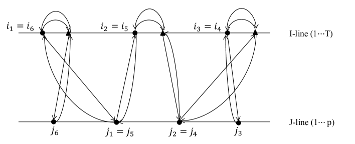
Figure 1: An example of the multigraph $Q(i,j)$ with $k=3$.

In the graph $Q(i,j)$, once a $I$-vertex $i_{l}$ is fixed, so is $i_{l}+s$. For this reason, we glue all the $I$-vertexes which are connected through horizon edges and denote the resulting graph as $M(A(t,s))$, where $A(t,s)$ is the index set that has $t$ distinct $I$-vertexes and $s$ distinct $J$-vertexes. An example of $M(A(3,4))$ that corresponds to the $Q(i,j)$ in Figure 1 is presented in the following Figure 2.

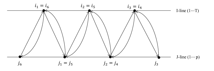
Figure 2: An example of $M(A(3,4))$ that corresponds to the $Q(i,j)$ in Figure 1.

2.2 Proof of Assertion (I)

Recall the expression of $m_{k}(A)$ in (2), we have

$$\mathbb{E}m_{k}(A) =\sum_{{\bf i}=1}^{T}\sum_{{\bf j}=1}^{p}\frac{1}{p^{k+1}T^{k}}\mathbb{E}\big{[}\varepsilon_{j_{1}\,i_{1}}\varepsilon_{j_{1}\,i_{2}}\varepsilon_{j_{2}\,s+i_{2}}\varepsilon_{j_{2}\,s+i_{3}}\varepsilon_{j_{3}\,i_{3}}\varepsilon_{j_{3}\,i_{4}}\varepsilon_{j_{4}\,s+i_{4}}\varepsilon_{j_{4}\,s+i_{5}}$$

$$\quad\quad\quad\quad\quad\quad\cdots\varepsilon_{j_{2k-1}\,i_{2k-1}}\varepsilon_{j_{2k-1}\,i_{2k}}\varepsilon_{j_{2k}\,s+i_{2k}}\varepsilon_{j_{2k}\,s+i_{1}}\big{]}$$

$$=\sum_{t,s}\frac{1}{p^{k+1}T^{k}}\sum_{M(A(t,s))}p(p-1)\cdots(p-s+1)T(T-1)\cdots(T-t+1)$$

$$\quad\quad\quad\quad\quad\quad\cdot\mathbb{E}\big{[}\varepsilon_{j_{1}\,i_{1}}\varepsilon_{j_{1}\,i_{2}}\varepsilon_{j_{2}\,s+i_{2}}\varepsilon_{j_{2}\,s+i_{3}}\cdots\varepsilon_{j_{2k-1}\,i_{2k}}\varepsilon_{j_{2k}\,s+i_{2k}}\varepsilon_{j_{2k}\,s+i_{1}}\big{]}$$

$$:=\sum_{t,s}S(t,s)\leavevmode\nobreak\ ,$$ (2.12)

where

$$S(t,s) =\frac{1}{p^{k+1}T^{k}}\sum_{M(A(t,s))}p(p-1)\cdots(p-s+1)T(T-1)\cdots(T-t+1)$$

$$\quad\quad\quad\quad\quad\quad\cdot\mathbb{E}\big{[}\varepsilon_{j_{1}\,i_{1}}\varepsilon_{j_{1}\,i_{2}}\cdots\varepsilon_{j_{2k}\,s+i_{2k}}\varepsilon_{j_{2k}\,s+i_{1}}\big{]}\leavevmode\nobreak\ .$$ (2.13)

Then we assert a lemma stating that $|S(t,s)|\rightarrow 0$ except for one particular term.

Lemma 2.1.

$|S(t,s)|\rightarrow 0$ as $p\rightarrow\infty$ unless $t=k$ and $s=k+1$.

Suppose Lemma 2.1 holds true for a moment, then according to (2.2) and (2.2), we have

$$\mathbb{E}m_{k}(A)=S(k,k+1)+o(1)=\mathbb{E}[\cdot]\cdot\#\{M(A(k,k+1))\}+o(1)\leavevmode\nobreak\ ,$$ (2.14)

where $\mathbb{E}[\cdot]$ refers to the expectation part in (2.2) and $\#\{M(A(k,k+1))\}$ refers to the number of isomorphism class that have $k$ distinct $I$-vertexes and $k+1$ distinct $J$-vertexes.

First, we show the expectation part $\mathbb{E}[\cdot]$ equals $1$ when $t=k$ and $s=k+1$. Let $v_{m}$ denote the number of edges in $M(A(t,s))$ whose degree is $m$. Then we have the total number of edges having the following relationship:

$$v_{1}+2v_{2}+\cdots+4kv_{4k}=4k\leavevmode\nobreak\ .$$ (2.15)

Since we have $\mathbb{E}\varepsilon_{ij}=0$ in (2.9), all the multiplicities of the edges in the graph $M(A(t,s))$ should be at least two, that is $v_{1}=0$. On the other hand, $M(A(t,s))$ is a connected graph with $t+s$ vertexes and $v_{1}+\cdots+v_{4k}$ ($=v_{2}+\cdots+v_{4k}$) edges, we have when $t=k$ and $s=k+1$:

$$2k+1=t+s \leq v_{1}+\cdots+v_{4k}+1=v_{2}+\cdots+v_{4k}+1$$

$$\leq\frac{1}{2}(2v_{2}+3v_{3}+\cdots+4kv_{4k})+1=2k+1\leavevmode\nobreak\ ,$$ (2.16)

where the last equality is due to (2.15) with $v_{1}=0$. Then we have all the inequalities in (2.2) become equalities, that is,

$$v_{2}+\cdots+v_{4k}+1=\frac{1}{2}(2v_{2}+3v_{3}+\cdots+4kv_{4k})+1=2k+1\leavevmode\nobreak\ ,$$

which leads to the fact that

$$v_{3}=v_{4}=\cdots=v_{4k}=0,\quad v_{2}=2k\leavevmode\nobreak\ .$$ (2.17)

This means that all the edges in the graph $M(A(k,k+1))$ is repeated exactly twice, so the part of expectation

$$\mathbb{E}\big{[}\varepsilon_{j_{1}\,i_{1}}\varepsilon_{j_{1}\,i_{2}}\cdots\varepsilon_{j_{2k}\,s+i_{2k}}\varepsilon_{j_{2k}\,s+i_{1}}\big{]}=\left(\mathbb{E}\varepsilon^{2}_{ji}\right)^{2k}=1\leavevmode\nobreak\ .$$ (2.18)

Second, the number of isomorphism class in $M(A(t,s))$ (with each edge repeated at least twice in the original graph $Q(i,j)$) is given by the notation $f_{t-1}(k)$ in Wang and Yao (2014), where

$$f_{t-1}(k)=\frac{1}{k}\begin{pmatrix}2k\\ t-1\\ \end{pmatrix}\begin{pmatrix}k\\ t\\ \end{pmatrix}\leavevmode\nobreak\ .$$

Therefore, in this special case when $t=k$ and $s=k+1$, we have

$$\#\{M(A(k,k+1))\}=f_{k-1}(k)=\frac{1}{k}\begin{pmatrix}2k\\ k-1\\ \end{pmatrix}\leavevmode\nobreak\ .$$ (2.19)

Finally, combine (2.14), (2.18) and (2.19), we have

$$\mathbb{E}m_{k}(A)=\frac{1}{k}\begin{pmatrix}2k\\ k-1\\ \end{pmatrix}+o(1)\leavevmode\nobreak\ .$$

Assertion (I) is then proved.

It remains to prove Lemma 2.1.

Proof.

(of Lemma 2.1) Denote $b_{l}$ as the degree that associated to the $I$-vertex $i_{l}$ $(1\leq l\leq t)$ in $M(A(t,s))$, then we have $b_{1}+\cdots+b_{t}=4k$, which is the total number of edges. On the other hand, since each edge in $M(A(t,s))$ is repeated at least twice (otherwise, there exist at least one single edge, so the expectation will be zero), we have each degree $b_{l}$ at least four (we glue the original $I$-vertexes $i_{l}$ and $i_{l}+s$ in $M(A(t,s))$). Therefore, we have

$$4k=b_{1}+\cdots+b_{t}\geq 4t\leavevmode\nobreak\ ,$$

which is $t\leq k$.

Now, consider the following two cases separately.

Case 1: $s>k+1$.

Recall the definition of $v_{m}$ in (2.15), which satisfies that

$$v_{1}+2v_{2}+\cdots+4kv_{4k}=2v_{2}+\cdots+4kv_{4k}=4k\leavevmode\nobreak\$$

and

$$t+s\leq v_{1}+\cdots+v_{4k}+1=v_{2}+\cdots+v_{4k}+1\leavevmode\nobreak\ .$$

We can bound the expectation part as follows:

$$\quad\Big{|}\mathbb{E}[\varepsilon_{j_{1}\,i_{1}}\varepsilon_{j_{1}\,i_{2}}\varepsilon_{j_{2}\,s+i_{2}}\varepsilon_{j_{2}\,s+i_{3}}\cdots\varepsilon_{j_{2k}\,s+i_{2k}}\varepsilon_{j_{2k}\,s+i_{1}}]\Big{|}$$

$$\leq\big{|}\mathbb{E}\varepsilon^{2}_{ji}\big{|}^{v_{2}}\cdots\big{|}\mathbb{E}\varepsilon^{4k}_{ji}\big{|}^{v_{4k}}\leq\left(\eta T^{1/4}\right)^{v_{3}+2v_{4}+\cdots+(4k-2)v_{4k}}$$

$$=\left(\eta T^{1/4}\right)^{3v_{3}+4v_{4}+\cdots+4kv_{4k}-2(v_{3}+v_{4}+\cdots+v_{4k})}$$

$$=\left(\eta T^{1/4}\right)^{4k-2(v_{2}+v_{3}+\cdots+v_{4k})}\leq\left(\eta T^{1/4}\right)^{4k-2(t+s-1)}\leavevmode\nobreak\ .$$ (2.20)

Then we have according to (2.2) that

$$|S(t,s)| \leq\frac{1}{p^{k+1}T^{k}}T^{t}p^{s}\left(\eta T^{1/4}\right)^{4k-2(t+s-1)}\#\{M(A(t,s))\}$$

$$=\frac{p^{s-k-1}}{T^{\frac{1}{2}(s-t-1)}}\eta^{4k-2(t+s-1)}\#\{M(A(t,s))\}$$

$$=O\left(\frac{p^{s-k-1}}{T^{\frac{1}{2}(s-t-1)}}\eta^{4k-2(t+s-1)}\right)\leavevmode\nobreak\ ,$$ (2.21)

where the last equality is due to the fact that $\#\{M(A(t,s))\}$ is a function of $k$ ($k$ is fixed), which could be bounded by a large enough constant.

Since $s>k+1$ and $t+s-1\leq 2k$, then

$$s-k-1-\frac{s}{2}+\frac{t}{2}+\frac{1}{2}=\frac{s}{2}-k+\frac{t}{2}-\frac{1}{2}=\frac{1}{2}(s+t-2k-1)\leq 0\leavevmode\nobreak\ ,$$

which is

$$0<s-k-1\leq\frac{1}{2}(s-t-1)\leavevmode\nobreak\ .$$

So, (2.2) reduces to

$$|S(t,k)|\leq O\left(\left(\frac{p}{T}\right)^{\frac{s-k-1}{2}}\eta^{4k-2(t+s-1)}\right)\rightarrow 0\leavevmode\nobreak\ ,$$ (2.22)

which is due to the fact that $s-k-1>0$ and $p/T\rightarrow 0$.

Case 2: $s\leq k+1$, but not $t=k$ and $s=k+1$.

For the same reason as before, we have $t$ distinct $I$-vertexes, each degree is at least four, so we have another estimation for the expectation part:

$$\bigg{|}\mathbb{E}[\varepsilon_{j_{1}\,i_{1}}\varepsilon_{j_{1}\,i_{2}}\varepsilon_{j_{2}\,s+i_{2}}\varepsilon_{j_{2}\,s+i_{3}}\cdots\varepsilon_{j_{2k}\,s+i_{2k}}\varepsilon_{j_{2k}\,s+i_{1}}]\bigg{|}\leq\left(\eta T^{1/4}\right)^{4k-4t}\leavevmode\nobreak\ .$$ (2.23)

Therefore,

$$|S(t,s)| \leq\frac{1}{p^{k+1}T^{k}}T^{t}p^{s}\left(\eta T^{1/4}\right)^{4k-4t}\#\{M(A(t,s))\}$$

$$=O\left(\frac{\eta^{4k-4t}}{p^{k+1-s}}\right)\leavevmode\nobreak\ ,$$ (2.24)

which is also due to the fact that $\#\{M(A(t,s))\}=O(1)$.

Case 2 contains three situations:

$$(1).\leavevmode\nobreak\ t=k\leavevmode\nobreak\ \text{and}\leavevmode\nobreak\ s<k+1:\displaystyle|S(t,s)|\leq O\left(\frac{1}{p^{k+1-s}}\right)\rightarrow 0\leavevmode\nobreak\ ;$$

$$(2).\leavevmode\nobreak\ t<k\leavevmode\nobreak\ \text{and}\leavevmode\nobreak\ s=k+1:\displaystyle|S(t,s)|\leq O\left(\eta^{4k-4t}\right)\rightarrow 0\leavevmode\nobreak\ ;$$

$$(3).\leavevmode\nobreak\ t<k\leavevmode\nobreak\ \text{and}\leavevmode\nobreak\ s<k+1:\displaystyle|S(t,s)|\leq O\left(\frac{\eta^{4k-4t}}{p^{k+1-s}}\right)\rightarrow 0\leavevmode\nobreak\ .$$ (2.25)

Combine (2.22) and (2.2), we have $|S(t,k)|\rightarrow 0$ as $p\rightarrow\infty$ unless

$$\left\{\begin{array}[]{l}t=k\\ s=k+1\leavevmode\nobreak\ .\end{array}\right.$$

∎

2.3 Proof of Assertion (II)

Recall

$$\quad\leavevmode\nobreak\ \mathop{\text{Var}}(m_{k}(A))$$

$$=\frac{1}{p^{2k+2}T^{2k}}\sum_{\bf{i_{1}},\bf{j_{1}},\bf{i_{2}},\bf{j_{2}}}\left[\mathbb{E}\left(\varepsilon_{Q(\bf{i_{1}},\bf{j_{1}})}\varepsilon_{Q(\bf{i_{2}},\bf{j_{2}})}\right)-\mathbb{E}\left(\varepsilon_{Q(\bf{i_{1}},\bf{j_{1}})}\right)\mathbb{E}\left(\varepsilon_{Q(\bf{i_{2}},\bf{j_{2}})}\right)\right]\leavevmode\nobreak\ .$$ (2.26)

If $Q(\bf{i_{1}},\bf{j_{1}})$ has no edges coincident with edges of $Q(\bf{i_{2}},\bf{j_{2}})$, then

$$\mathbb{E}\left(\varepsilon_{Q(\bf{i_{1}},\bf{j_{1}})}\varepsilon_{Q(\bf{i_{2}},\bf{j_{2}})}\right)-\mathbb{E}\left(\varepsilon_{Q(\bf{i_{1}},\bf{j_{1}})}\right)\mathbb{E}\left(\varepsilon_{Q(\bf{i_{2}},\bf{j_{2}})}\right)=0$$

by independence between $\varepsilon_{Q(\bf{i_{1}},\bf{j_{1}})}$ and $\varepsilon_{Q(\bf{i_{2}},\bf{j_{2}})}$. If $Q=Q({\bf{i_{1}},\bf{j_{1}}})\bigcup Q({\bf{i_{2}},\bf{j_{2}}})$ has an overall single edge, then

$$\mathbb{E}\left(\varepsilon_{Q(\bf{i_{1}},\bf{j_{1}})}\varepsilon_{Q(\bf{i_{2}},\bf{j_{2}})}\right)=\mathbb{E}\left(\varepsilon_{Q(\bf{i_{1}},\bf{j_{1}})}\right)\mathbb{E}\left(\varepsilon_{Q(\bf{i_{2}},\bf{j_{2}})}\right)=0\leavevmode\nobreak\ ,$$

so in the above two cases, we have $\mathop{\text{Var}}(m_{k}(A))=0$.

Now, suppose $Q=Q({\bf{i_{1}},\bf{j_{1}}})\bigcup Q({\bf{i_{2}},\bf{j_{2}}})$ has no single edge, $Q({\bf{i_{1}},\bf{j_{1}}})$ and $Q({\bf{i_{2}},\bf{j_{2}}})$ have common edges. Let the number of vertexes of $Q({\bf{i_{1}},\bf{j_{1}}})$, $Q({\bf{i_{2}},\bf{j_{2}}})$, $Q=Q({\bf{i_{1}},\bf{j_{1}}})\bigcup Q({\bf{i_{2}},\bf{j_{2}}})$ on the $I$-line be $t_{1}$, $t_{2}$, $t$, respectively; and the number of vertexes on the $J$-line be $s_{1}$, $s_{2}$, $s$, respectively. Since $Q({\bf{i_{1}},\bf{j_{1}}})$ and $Q({\bf{i_{2}},\bf{j_{2}}})$ have common edges, we must have $t\leq t_{1}+t_{2}-1$, $s\leq s_{1}+s_{2}-1$.

Similar to (2.2) and (2.23), we have two bounds for $\left|\mathbb{E}\left(\varepsilon_{Q(\bf{i_{1}},\bf{j_{1}})}\varepsilon_{Q(\bf{i_{2}},\bf{j_{2}})}\right)\right|$:

$$\left|\mathbb{E}\left(\varepsilon_{Q(\bf{i_{1}},\bf{j_{1}})}\varepsilon_{Q(\bf{i_{2}},\bf{j_{2}})}\right)\right|\leq\left(\eta T^{1/4}\right)^{8k-2(t+s-1)}\leavevmode\nobreak\ ,$$ (2.27)

or

$$\left|\mathbb{E}\left(\varepsilon_{Q(\bf{i_{1}},\bf{j_{1}})}\varepsilon_{Q(\bf{i_{2}},\bf{j_{2}})}\right)\right|\leq\left(\eta T^{1/4}\right)^{8k-4t}\leavevmode\nobreak\ .$$ (2.28)

For the same reason, we have also

$$\left|\mathbb{E}\varepsilon_{Q(\bf{i_{1}},\bf{j_{1}})}\mathbb{E}\varepsilon_{Q(\bf{i_{2}},\bf{j_{2}})}\right| \leq\left(\eta T^{1/4}\right)^{4k-2(t_{1}+s_{1}-1)+4k-2(t_{2}+s_{2}-1)}$$

$$<\left(\eta T^{1/4}\right)^{8k-2(t+s-1)}\leavevmode\nobreak\ ,$$ (2.29)

or

$$\left|\mathbb{E}\left(\varepsilon_{Q(\bf{i_{1}},\bf{j_{1}})}\varepsilon_{Q(\bf{i_{2}},\bf{j_{2}})}\right)\right|\leq\left(\eta T^{1/4}\right)^{4k-4t_{1}+4k-4t_{2}}<\left(\eta T^{1/4}\right)^{8k-4t}\leavevmode\nobreak\ ,$$ (2.30)

where the last inequalities in (2.3) and (2.30) are due to the fact that $t\leq t_{1}+t_{2}-1$, $s\leq s_{1}+s_{2}-1$.

Since

$$\quad\leavevmode\nobreak\ \mathop{\text{Var}}(m_{k}(A))$$

$$=\frac{1}{p^{2k+2}T^{2k}}\sum_{t,s}\sum_{M(A(t,s))}\left[\mathbb{E}\left(\varepsilon_{Q(\bf{i_{1}},\bf{j_{1}})}\varepsilon_{Q(\bf{i_{2}},\bf{j_{2}})}\right)-\mathbb{E}\left(\varepsilon_{Q(\bf{i_{1}},\bf{j_{1}})}\right)\mathbb{E}\left(\varepsilon_{Q(\bf{i_{2}},\bf{j_{2}})}\right)\right]$$

$$:=\sum_{t,s}\widetilde{S}(t,s)\leavevmode\nobreak\ .$$ (2.31)

Using (2.27), (2.28), (2.3) and (2.30), we can bound the value of $|\widetilde{S}(t,s)|$ as follows:

$$|\widetilde{S}(t,s)| \leq O\left(\frac{T^{t}p^{s}}{p^{2k+2}T^{2k}}\left(\eta T^{1/4}\right)^{8k-2(t+s-1)}\right)$$

$$=O\left(\frac{p^{s-2k-2}}{T^{s/2-t/2-1/2}}\right)\leavevmode\nobreak\ ,$$ (2.32)

or

$$|\widetilde{S}(t,s)| \leq O\left(\frac{T^{t}p^{s}}{p^{2k+2}T^{2k}}\left(\eta T^{1/4}\right)^{8k-4t}\right)$$

$$=O\left(p^{s-2k-2}\right)\leavevmode\nobreak\ .$$ (2.33)

Clearly,

$$t_{1}+s_{1}\leq 2k+1\leavevmode\nobreak\ ,\quad t_{2}+s_{2}\leq 2k+1\leavevmode\nobreak\ ;$$

we have thus

$$t+s\leq t_{1}+t_{2}-1+s_{1}+s_{2}-1\leq 4k\leavevmode\nobreak\ .$$

First, consider the case that $s>t+1$ where we use the bound in (2.3). Since

$$s-2k-2-s/2+t/2+1/2=s/2+t/2-2k-3/2\leq-3/2\leavevmode\nobreak\ ,$$

which leads to

$$s-2k-2\leq-3/2+s/2-t/2-1/2\leavevmode\nobreak\ .$$

Combine with (2.3), we have

$$|\widetilde{S}(t,s)| \leq O\left(p^{-3/2}\left(\frac{p}{T}\right)^{\frac{1}{2}(s-t-1)}\right)\leq O\left(p^{-3/2}\right)\leavevmode\nobreak\ .$$ (2.34)

Second, we use the bound in (2.3) for the case $s\leq t+1$. Recall that $t+s\leq 4k$, we have

$$s-1+s\leq t+s\leq 4k\leavevmode\nobreak\ ,$$

which is

$$2s-1\leq 4k\leavevmode\nobreak\ .$$

Then, from (2.3),

$$|\widetilde{S}(t,s)| \leq O\left(p^{s-2k-2}\right)\leq O\left(p^{\frac{4k+1}{2}-2k-2}\right)=O\left(p^{-3/2}\right)\leavevmode\nobreak\ .$$ (2.35)

Combine (2.3), (2.34) and (2.35), we have

$$\big{|}\mathop{\text{Var}}(m_{k}(A))\big{|}\leq C(k)p^{-3/2}\leavevmode\nobreak\ ,$$

which is summable with respect to $p$. Assertion (II) is then proved.

3 Convergence of the largest eigenvalue of $A$

In this section, we aim to show that the largest eigenvalue of $A$ tends to 4 almost surely, which is the right edge of its LSD.

Theorem 3.1.

Under the same conditions as in Theorem 2.1, with $\sup_{it}\mathbb{E}(\varepsilon_{it}^{4})<\infty$ in (2.1) replaced by $\sup_{it}\mathbb{E}(|\varepsilon_{it}|^{4+\nu})<\infty$ for some $\nu>0$, the largest eigenvalue of $A$ converges to $4$ almost surely.

Recall that in the proof of Theorem 2.2, a main step is Lemma 2.1, which says that $|S(t,s)|\rightarrow 0$ except for one term, which is when $t=k$ and $s=k+1$. One thing to mention here is that in order to prove this lemma, $k$ is assumed to be fixed. Then the number of isomorphism class in $M(A(t,s))$ is a function of $k$, thus can be bounded by a large enough constant. So actually, we do not need to know the value of $\#\{M(A(t,s))\}$ exactly. While in the case of deriving the convergence of the largest eigenvalue, $k$ should grow to infinity, so we can not trivially guarantee that the number of isomorphism class in $M(A(t,s))$ is still of constant order. Therefore, the main task in this section is to bound this value, making $|S(t,s)|$ ($t\neq k$ or $s\neq k+1$) still a smaller order compared with the main term $|S(k,k+1)|$ when $k\rightarrow\infty$.

Proposition 3.1.

Let the conditions in Theorem 2.1 hold, with $\sup_{it}\mathbb{E}(\varepsilon_{it}^{4})<\infty$ in (2.1) replaced by $\sup_{it}\mathbb{E}(|\varepsilon_{it}|^{4+\nu})<\infty$ for some $\nu>0$, and $k=k(p,T)$ is an integer that tends to infinity and satisfies the following conditions:

$$\left\{\begin{array}[]{l}k/\log p\rightarrow\infty,\\ kp/T\rightarrow 0,\\ k/p\rightarrow.0\\ \end{array}\right.$$ (3.4)

Then we have

$$\mathbb{E}(m_{k}(A_{T})) =\frac{1}{k}\left(\begin{array}[]{c}2k\\ k-1\end{array}\right)\cdot(1+o_{k}(1))\leavevmode\nobreak\ .$$

Now suppose the above Proposition 3.1 holds true. We first show it will lead to Theorem 3.1.

Proof.

(of Theorem 3.1) Using Proposition 3.1, we have the estimation that

$$\mathbb{E}(m_{k}(A))=\frac{1}{k}\left(\begin{array}[]{c}2k\\ k-1\end{array}\right)\cdot(1+o_{k}(1))\leavevmode\nobreak\ ,$$ (3.7)

then for any $\Delta>0$, we have

$$\quad\leavevmode\nobreak\ P(l_{1}>4+\Delta)\leq P(\mathop{\text{tr}}A^{k}\geq(4+\Delta)^{k})\leq\frac{\mathbb{E}\mathop{\text{tr}}A^{k}}{(4+\Delta)^{k}}=\frac{p\cdot\mathbb{E}(m_{k}(A))}{(4+\Delta)^{k}}$$

$$\leq\frac{p}{(4+\Delta)^{k}}\cdot\frac{1}{k}\left(\begin{array}[]{c}2k\\ k-1\end{array}\right)\cdot(1+o_{k}(1))\leq\left(\frac{4p^{1/k}}{4+\Delta}\right)^{k}\cdot(1+o_{k}(1))\leavevmode\nobreak\ .$$ (3.10)

The right hand side tends to $\left(\frac{4}{4+\Delta}\right)^{k}$ since $k/\log p\rightarrow\infty$ (so $p^{1/k}\rightarrow 1$). Once we fix this $\Delta>0$, (3) is summable.

The upper bound for $l_{1}$ is trivial due to our Theorem 2.2. ∎

Now it remains to prove our Proposition 3.1.

Proof.

(of Proposition 3.1) After truncation, centralisation and rescaling, we may assume that the $\varepsilon_{it}$’s satisfy the condition that

$$\ E(\varepsilon_{it})=0,\leavevmode\nobreak\ \mathop{\text{Var}}(\varepsilon_{it})=1,\leavevmode\nobreak\ |\varepsilon_{it}|\leq\delta T^{1/2}\leavevmode\nobreak\ ,$$ (3.11)

where $\delta$ is chosen such that

$$\left\{\begin{array}[]{l}\delta\rightarrow 0\\ \delta T^{1/2-\epsilon}\rightarrow 0\\ \delta T^{1/2}\rightarrow\infty\\ \delta^{2}k\sqrt{T}\rightarrow 0\\ \frac{kp}{\delta^{2}T}\rightarrow\infty\leavevmode\nobreak\ .\end{array}\right.$$ (3.17)

More detailed justifications of (3.11) are provided in Appendix B.

From the proof of Theorem 2.2, we have

$$\mathbb{E}m_{k}(A)=\sum_{t,s}S(t,s)=S(k,k+1)+o(1)=\frac{1}{k}\begin{pmatrix}2k\\ k-1\\ \end{pmatrix}+o(1)\leavevmode\nobreak\ ,$$

where $S(k,k+1)$ is the main term that contributes to $\mathbb{E}m_{k}(A)$, while all other terms can be neglect. Therefore, it remains to prove that when $k\rightarrow\infty$, we still have

$$\sum_{t\neq k\leavevmode\nobreak\ \text{or}\leavevmode\nobreak\ s\neq k+1}S(t,s)=\frac{1}{k}\begin{pmatrix}2k\\ k-1\\ \end{pmatrix}\cdot o_{k}(1)\leavevmode\nobreak\ .$$

We also consider two cases:

$\begin{array}[]{l}\text{Case 1}:s>k+1\\[5.69054pt] \text{Case 2}:s\leq k+1,\leavevmode\nobreak\ \text{but not}\leavevmode\nobreak\ t=k\leavevmode\nobreak\ \text{and}\leavevmode\nobreak\ s=k+1.\end{array}$

Similar to (2.2) and (2.23), we have two bounds for the expectation part:

$$\Big{|}\mathbb{E}[\varepsilon_{j_{1}\,i_{1}}\varepsilon_{j_{1}\,i_{2}}\varepsilon_{j_{2}\,s+i_{2}}\varepsilon_{j_{2}\,s+i_{3}}\cdots\varepsilon_{j_{2k}\,s+i_{2k}}\varepsilon_{j_{2k}\,s+i_{1}}]\Big{|}\leq\left(\delta T^{1/2}\right)^{4k-2(t+s-1)}\leavevmode\nobreak\$$ (3.18)

or

$$\bigg{|}\mathbb{E}[\varepsilon_{j_{1}\,i_{1}}\varepsilon_{j_{1}\,i_{2}}\varepsilon_{j_{2}\,s+i_{2}}\varepsilon_{j_{2}\,s+i_{3}}\cdots\varepsilon_{j_{2k}\,s+i_{2k}}\varepsilon_{j_{2k}\,s+i_{1}}]\bigg{|}\leq\left(\delta T^{1/2}\right)^{4k-4t}\leavevmode\nobreak\ .$$ (3.19)

Consider $t=1$ first. From Wang et al. (2013), the number of isomorphism class $\#\{M(A(1,s))\}$ is bounded by

$$\begin{pmatrix}2k\\ 2k-s\\ \end{pmatrix}\leavevmode\nobreak\ ,$$

and combine this with (2.2) and (3.18), we have

$$|S(1,s)|\leq\frac{1}{p^{k+1}T^{k}}Tp^{s}\left(\delta T^{1/2}\right)^{4k-2s}\left(\begin{array}[]{c}2k\\ 2k-s\end{array}\right)\leavevmode\nobreak\ .$$ (3.22)

Then,

$$\big{|}\sum_{s}S(1,s)\big{|} \leq\sum_{s=1}^{2k}\frac{1}{p^{k+1}T^{k}}Tp^{s}\left(\delta T^{1/2}\right)^{4k-2s}\left(\begin{array}[]{c}2k\\ 2k-s\end{array}\right)$$ (3.25)

$$=\sum_{s=1}^{2k}\frac{1}{p^{k+1}T^{k}}Tp^{s}\left(\delta T^{1/2}\right)^{4k-2s}\left(\begin{array}[]{c}2k\\ s\end{array}\right)\leavevmode\nobreak\ .$$ (3.28)

The right hand side of (3.25) can be bounded as

$$\sum_{s=1}^{2k}\frac{T}{p^{k+1}T^{k}}\left(\delta T^{1/2}\right)^{4k}\left(\frac{2kp}{\delta^{2}T}\right)^{s}\leavevmode\nobreak\ ,$$

which is dominated by the term when $s=2k$ since $\frac{kp}{\delta^{2}T}\rightarrow\infty$. Then (3.25) reduces to

$$\frac{1}{p^{k+1}T^{k}}Tp^{2k}=\left(\frac{p}{T}\right)^{k-1}\rightarrow 0\leavevmode\nobreak\ .$$ (3.29)

Next, we consider Case 1 and Case 2 (when $t>1$) separately. According to Wang et al. (2013), the number of isomorphism class in $M(A(s,t))$ ($t>1$) is bounded by

$$f_{t-1}(k)\left(\begin{array}[]{c}2k-t\\ s-1\end{array}\right)\leavevmode\nobreak\ ,$$ (3.32)

where

$$f_{t-1}(k)=\frac{1}{k}\begin{pmatrix}2k\\ t-1\\ \end{pmatrix}\begin{pmatrix}k\\ t\\ \end{pmatrix}\leavevmode\nobreak\ .$$

Case 1 ($s>k+1$ and $t>1$): The part of expectation can be bounded by (3.18), and combining this with (2.2) and (3.32), we have

$$|S(t,s)| \leq\frac{1}{p^{k+1}T^{k}}\sum_{M(A(t,s))}p^{s}T^{t}\cdot\Big{|}\mathbb{E}[\varepsilon_{j_{1}\,i_{1}}\varepsilon_{j_{1}\,i_{2}}\cdots\varepsilon_{j_{2k}\,s+i_{2k}}\varepsilon_{j_{2k}\,s+i_{1}}]\Big{|}$$

$$\leq\frac{p^{s}T^{t}}{p^{k+1}T^{k}}\left(\delta T^{1/2}\right)^{4k-2(t+s-1)}\cdot f_{t-1}(k)\left(\begin{array}[]{c}2k-t\\ s-1\end{array}\right)\leavevmode\nobreak\ .$$ (3.35)

Since $s\geq k+2$, $t\geq 2$, and a trivial relationship that $t+s-1\leq 2k$, we have

$$\Big{|}\sum_{t,s}S(t,s)\Big{|} \leq\sum_{t=2}^{k-1}\sum_{s=k+2}^{2k+1-t}\frac{p^{s}T^{t}}{p^{k+1}T^{k}}\left(\delta T^{1/2}\right)^{4k-2(t+s-1)}\cdot f_{t-1}(k)\left(\begin{array}[]{c}2k-t\\ s-1\end{array}\right)\leavevmode\nobreak\ .$$ (3.38)

The summation over $s$ in (3.38) can be bounded as follows:

$$\sum_{s=k+2}^{2k+1-t}\delta^{-2s}T^{-s}p^{s}\left(\begin{array}[]{c}2k-t\\ s-1\end{array}\right)\leq\sum_{s=k+2}^{2k+1-t}\left(\frac{2kp}{\delta^{2}T}\right)^{s}\leavevmode\nobreak\ ,$$ (3.41)

and since $\frac{kp}{\delta^{2}T}\rightarrow\infty$, the summation in (3.41) is dominated by the term of $s=2k+1-t$. Therefore, (3.38) reduces to

$$\quad\sum_{t=2}^{k-1}\frac{p^{2k+1-t}T^{t}}{p^{k+1}T^{k}}\left(\delta T^{1/2}\right)^{4k-2(t+2k+1-t-1)}\cdot f_{t-1}(k)\left(\begin{array}[]{c}2k-t\\ 2k+1-t-1\end{array}\right)$$ (3.44)

$$=\sum_{t=2}^{k-1}\left(\frac{p}{T}\right)^{k-t}f_{t-1}(k)=\sum_{t=2}^{k-1}\frac{1}{k}\left(\begin{array}[]{c}2k\\ t-1\end{array}\right)\left(\begin{array}[]{c}k\\ t\end{array}\right)\left(\frac{p}{T}\right)^{k-t}\leavevmode\nobreak\ .$$ (3.49)

For the same reason, the right hand side of (3.44) inside the summation can be bounded by

$$\frac{1}{k}\left(\frac{p}{T}\right)^{k}\left(\frac{2k^{2}T}{p}\right)^{t}\leavevmode\nobreak\ ,$$

and since $Tk^{2}/p=k^{2}/(\frac{p}{T})\rightarrow\infty$, the dominating term in (3.44) is when $t=k-1$, which reduces to

$$\frac{1}{k}\left(\begin{array}[]{c}2k\\ k-2\end{array}\right)\left(\begin{array}[]{c}k\\ k-1\end{array}\right)\left(\frac{p}{T}\right)=\frac{k(k-1)}{k+2}\frac{p}{T}\cdot\frac{1}{k}\left(\begin{array}[]{c}2k\\ k-1\end{array}\right)\leavevmode\nobreak\ .$$ (3.56)

Since $kp/T\rightarrow 0$, we have (3.56) equals

$$\frac{1}{k}\left(\begin{array}[]{c}2k\\ k-1\end{array}\right)\cdot o_{k}(1)\leavevmode\nobreak\ .$$ (3.59)

Therefore, in this case, we have

$$\Big{|}\sum_{t,s}S(t,s)\Big{|}=\frac{1}{k}\left(\begin{array}[]{c}2k\\ k-1\end{array}\right)\cdot o_{k}(1)\leavevmode\nobreak\ .$$ (3.62)

Case 2 ($2\leq t\leq k$ and $s\leq k+1$): For the same reason, combining the bound of the expectation part in (3.19) with (2.2) and (3.32), we have

$$|S(t,s)| =\frac{1}{p^{k+1}T^{k}}\sum_{M(A(t,s))}p^{s}T^{t}\cdot\Big{|}\mathbb{E}[\varepsilon_{j_{1}\,i_{1}}\varepsilon_{j_{1}\,i_{2}}\cdots\varepsilon_{j_{2k}\,s+i_{2k}}\varepsilon_{j_{2k}\,s+i_{1}}]\Big{|}$$

$$\leq\frac{1}{p^{k+1}T^{k}}\left(\delta T^{1/2}\right)^{4k-4t}\cdot p^{s}T^{t}\cdot f_{t-1}(k)\left(\begin{array}[]{c}2k-t\\ s-1\end{array}\right)\leavevmode\nobreak\ .$$ (3.65)

Therefore, we have

$$\Big{|}\sum_{t,s}S(t,s)\Big{|}\leq\sum_{t=2}^{k}\sum_{s=1}^{k+1}p^{s-k-1}T^{k-t}\delta^{4k-4t}f_{t-1}(k)\left(\begin{array}[]{c}2k-t\\ s-1\end{array}\right)\leavevmode\nobreak\ .$$ (3.68)

We also consider the following three situations:

$$(1).\leavevmode\nobreak\ t=k\leavevmode\nobreak\ \text{and}\leavevmode\nobreak\ s<k+1\leavevmode\nobreak\ ,$$

$$(2).\leavevmode\nobreak\ 1<t<k\leavevmode\nobreak\ \text{and}\leavevmode\nobreak\ s=k+1\leavevmode\nobreak\ ,$$

$$(3).\leavevmode\nobreak\ 1<t<k\leavevmode\nobreak\ \text{and}\leavevmode\nobreak\ s<k+1\leavevmode\nobreak\ ,$$

and show that for all the above three situations, we have (3.68) bounded by

$$\frac{1}{k}\begin{pmatrix}2k\\ k-1\\ \end{pmatrix}\cdot o_{k}(1)\leavevmode\nobreak\ .$$

For situation (1), (3.68) reduces to

$$\sum_{s=1}^{k}p^{s-k-1}f_{k-1}(k)\left(\begin{array}[]{c}k\\ s-1\end{array}\right)=\sum_{s=1}^{k}p^{s-k-1}\frac{1}{k}\left(\begin{array}[]{c}2k\\ k-1\end{array}\right)\left(\begin{array}[]{c}k\\ s-1\end{array}\right)\leavevmode\nobreak\ ,$$ (3.75)

which can be bounded as

$$\sum_{s=1}^{k}p^{-k-1}\frac{1}{k}\begin{pmatrix}2k\\ k-1\\ \end{pmatrix}(kp)^{s}\leavevmode\nobreak\ .$$

Therefore, the dominating term is when $s=k$, thus (3.75) reduces to

$$\frac{1}{k}\begin{pmatrix}2k\\ k-1\\ \end{pmatrix}\cdot\frac{k}{p}=\frac{1}{k}\begin{pmatrix}2k\\ k-1\\ \end{pmatrix}\cdot o_{k}(1)\leavevmode\nobreak\ ,$$

which is due to the choice of $k$ that $k/p\rightarrow 0$.

For situation (2), (3.68) reduces to

$$\leavevmode\nobreak\ \quad\sum_{t=2}^{k-1}\delta^{4k-4t}T^{k-t}\cdot f_{t-1}(k)\left(\begin{array}[]{c}2k-t\\ k\end{array}\right)$$ (3.78)

$$=\sum_{t=2}^{k-1}\delta^{4k-4t}T^{k-t}\cdot\frac{1}{k}\left(\begin{array}[]{c}2k\\ t-1\end{array}\right)\left(\begin{array}[]{c}k\\ t\end{array}\right)\left(\begin{array}[]{c}2k-t\\ k\end{array}\right)\leavevmode\nobreak\ .$$ (3.85)

Since the right hand side of (3.78) can be bounded by

$$\sum_{t=2}^{k-1}\delta^{4k}\cdot\frac{(2kT)^{k}}{k}\left(\frac{2k^{2}}{\delta^{4}T}\right)^{t}\leavevmode\nobreak\ ,$$ (3.86)

which is dominated by the term of $t=k-1$ since $\frac{2k^{2}}{T\delta^{4}}=\frac{2k^{2}}{(\delta T^{1/4})^{4}}\rightarrow\infty$. Therefore, we have (3.78) bounded by

$$\leavevmode\nobreak\ \quad T\delta^{4}\cdot\frac{1}{k}\left(\begin{array}[]{c}2k\\ k-2\end{array}\right)\left(\begin{array}[]{c}k\\ k-1\end{array}\right)\left(\begin{array}[]{c}k+1\\ k\end{array}\right)\leavevmode\nobreak\$$

$$=\delta^{4}T\frac{(k-1)k(k+1)}{k+2}\cdot\frac{1}{k}\left(\begin{array}[]{c}2k\\ k-1\end{array}\right)$$

$$\rightarrow\frac{1}{k}\left(\begin{array}[]{c}2k\\ k-1\end{array}\right)\cdot o_{k}(1)\leavevmode\nobreak\ ,$$

which is due to the fact that $\delta^{4}Tk^{2}=(\delta^{2}\sqrt{T}k)^{2}\rightarrow 0$.

For situation (3), we have (3.68) reduce to

$$\leavevmode\nobreak\ \quad\sum_{t=2}^{k-1}\sum_{s=1}^{k}p^{s-k-1}T^{k-t}\delta^{4k-4t}\cdot f_{t-1}(k)\left(\begin{array}[]{c}2k-t\\ s-1\end{array}\right)$$ (3.89)

$$=\sum_{t=2}^{k-1}\sum_{s=1}^{k}p^{s-k-1}T^{k-t}\delta^{4k-4t}\cdot\frac{1}{k}\left(\begin{array}[]{c}2k\\ t-1\end{array}\right)\left(\begin{array}[]{c}k\\ t\end{array}\right)\left(\begin{array}[]{c}2k-t\\ s-1\end{array}\right)\leavevmode\nobreak\ .$$ (3.96)

The part of summation over $s$ is

$$\sum_{s=1}^{k}p^{s}\left(\begin{array}[]{c}2k-t\\ s-1\end{array}\right)\leavevmode\nobreak\ ,$$

which could be bounded by

$$\sum_{s=1}^{k}(2kp)^{s}\leavevmode\nobreak\ ,$$

therefore, the dominating term is when $s=k$. So (3.89) reduces to

$$\sum_{t=2}^{k-1}p^{-1}\delta^{4k-4t}T^{k-t}\cdot\frac{1}{k}\left(\begin{array}[]{c}2k\\ t-1\end{array}\right)\left(\begin{array}[]{c}k\\ t\end{array}\right)\left(\begin{array}[]{c}2k-t\\ k-1\end{array}\right)\leavevmode\nobreak\ .$$ (3.103)

For the same reason, the right hand side of (3.103) can be bounded by

$$\sum_{t=2}^{k-1}p^{-1}\delta^{4k}\cdot\frac{1}{k}\left(\frac{2k^{2}}{T\delta^{4}}\right)^{t}(2kT)^{k}\leavevmode\nobreak\ ,$$

which is dominated by the term of $t=k-1$ since $\frac{k^{2}}{T\delta^{4}}=\frac{k^{2}}{\left(\delta T^{1/4}\right)^{4}}\rightarrow\infty$. Therefore, (3.103) reduces to

$$\frac{T}{p}\delta^{4}\cdot\frac{1}{k}\left(\begin{array}[]{c}2k\\ k-2\end{array}\right)\left(\begin{array}[]{c}k\\ k-1\end{array}\right)\left(\begin{array}[]{c}k+1\\ k-1\end{array}\right)=O\left(\frac{\delta^{4}k^{3}T}{p}\cdot\frac{1}{k}\left(\begin{array}[]{c}2k\\ k-1\end{array}\right)\right)\leavevmode\nobreak\ ,$$ (3.112)

and since $\frac{\delta^{4}k^{3}T}{p}=(\delta^{2}k\sqrt{T})^{2}\cdot k/p\rightarrow 0$, we have (3.112) equals

$$\frac{1}{k}\left(\begin{array}[]{c}2k\\ k-1\end{array}\right)\cdot o_{k}(1)\leavevmode\nobreak\ .$$

Finally, in all the three situations, we have

$$\Big{|}\sum_{t,s}S(t,s)\Big{|}=\frac{1}{k}\left(\begin{array}[]{c}2k\\ k-1\end{array}\right)\cdot o_{k}(1)\leavevmode\nobreak\ .$$

The proof of Proposition 3.1 is complete.

∎

Appendix A Justification of truncation, centralisation and rescaling in (2.9)

A.1 Truncation

Define two $p\times T$ matrices

$$E_{1}:=(\varepsilon_{1}\leavevmode\nobreak\ \varepsilon_{2}\cdots\leavevmode\nobreak\ \varepsilon_{T-1}\leavevmode\nobreak\ \varepsilon_{T})\leavevmode\nobreak\ ,\quad E_{2}:=(\varepsilon_{s+1}\leavevmode\nobreak\ \varepsilon_{s+2}\cdots\leavevmode\nobreak\ \varepsilon_{s+T-1}\leavevmode\nobreak\ \varepsilon_{s+T})\leavevmode\nobreak\ ,$$ (A.1)

then

$$X_{T}=\frac{1}{T}\sum_{t=s+1}^{s+T}\varepsilon_{t}\varepsilon^{T}_{t-s}=\frac{1}{T}E_{2}E_{1}^{T}\leavevmode\nobreak\ ,$$ (A.2)

and our target matrix

$$A=\frac{T}{p}X_{T}X_{T}^{T}=\frac{1}{pT}E_{2}E_{1}^{T}E_{1}E_{2}^{T}\leavevmode\nobreak\ .$$ (A.3)

Let

$$\hat{\varepsilon}_{ij}=\varepsilon_{ij}\mathbf{1}_{\{|\varepsilon_{ij}|\leq\eta T^{1/4}\}}\leavevmode\nobreak\ ,$$

$\hat{X}_{T}$ and $\hat{A}$ are defined by replacing all the $\varepsilon_{ij}$ with $\hat{\varepsilon}_{ij}$ in (A.2) and (A.3).

Using Theorem A.44 in Bai and Silverstein (2010) and the inequality that

$$\text{rank}(AB-CD)\leq\text{rank}(A-C)+\text{rank}(B-D)\leavevmode\nobreak\ ,$$

we have

$$\quad\left\|F^{A}(x)-F^{\hat{A}}(x)\right\|=\left\|F^{\frac{T}{p}X_{T}X^{T}_{T}}(x)-F^{\frac{T}{p}\hat{X}_{T}\hat{X}^{T}_{T}}(x)\right\|$$

$$\leq\frac{1}{p}\text{rank}\left(\sqrt{\frac{T}{p}}X_{T}-\sqrt{\frac{T}{p}}\hat{X}_{T}\right)=\frac{1}{p}\text{rank}\left(X_{T}-\hat{X}_{T}\right)$$

$$=\frac{1}{p}\text{rank}\left(\frac{1}{T}E_{2}E^{T}_{1}-\frac{1}{T}\hat{E}_{2}\hat{E}^{T}_{1}\right)=\frac{1}{p}\text{rank}\left(E_{2}E^{T}_{1}-\hat{E}_{2}\hat{E}^{T}_{1}\right)$$

$$\leq\frac{1}{p}\text{rank}\left(E_{2}-\hat{E}_{2}\right)+\frac{1}{p}\text{rank}\left(E_{1}-\hat{E}_{1}\right)$$

$$=\frac{2}{p}\text{rank}\left(E_{1}-\hat{E}_{1}\right)\leq\frac{2}{p}\sum_{i=1}^{p}\sum_{j=1}^{T}\mathbf{1}_{\{|\varepsilon_{ij}|>\eta T^{1/4}\}}\leavevmode\nobreak\ .$$ (A.4)

Since $\sup_{it}\mathbb{E}(\varepsilon_{it}^{4})<\infty$, we have always

$$\frac{1}{\eta^{4}pT}\sum_{i,j}\mathbb{E}\left(|\varepsilon_{ij}|^{4}I_{(|\varepsilon_{ij}|>\eta T^{1/4})}\right)\longrightarrow 0\leavevmode\nobreak\ \quad\text{as}\leavevmode\nobreak\ p,T\rightarrow\infty\leavevmode\nobreak\ .$$

Consider the expectation and variance of $\frac{1}{p}\sum_{i=1}^{p}\sum_{j=1}^{T}\mathbf{1}_{\{|\varepsilon_{ij}|>\eta T^{1/4}\}}$ in (A.1):

$$\mathbb{E}\bigg{(}\frac{2}{p}\sum_{i=1}^{p}\sum_{j=1}^{T}\mathbf{1}_{\{|\varepsilon_{ij}|>\eta T^{1/4}\}}\bigg{)} \leq\frac{2}{p}\sum_{i=1}^{p}\sum_{j=1}^{T}\frac{\mathbb{E}\Big{(}|\varepsilon_{ij}|^{4}\cdot\mathbf{1}_{\{|\varepsilon_{ij}|>\eta T^{1/4}\}}\Big{)}}{\eta^{4}T}=o(1)\leavevmode\nobreak\ ,$$

$$\mathop{\text{Var}}\bigg{(}\frac{2}{p}\sum_{i=1}^{p}\sum_{j=1}^{T}\mathbf{1}_{\{|\varepsilon_{ij}|>\eta T^{1/4}\}}\bigg{)} \leq\frac{4}{p^{2}}\sum_{i=1}^{p}\sum_{j=1}^{T}\frac{\mathbb{E}\Big{(}|\varepsilon_{ij}|^{4}\cdot\mathbf{1}_{\{|\varepsilon_{ij}|>\eta T^{1/4}\}}\Big{)}}{\eta^{4}T}=o(\frac{1}{p})\leavevmode\nobreak\ .$$

Applying Bernstein’s inequality, for all small $\varepsilon>0$ and large $p$, we have

$$P\left(\frac{2}{p}\sum_{i=1}^{p}\sum_{j=1}^{T}\mathbf{1}_{\{|\varepsilon_{ij}|>\eta T^{1/4}\}}\geq\varepsilon\right)\leq 2e^{-\frac{1}{2}\varepsilon^{2}p}\leavevmode\nobreak\ .$$ (A.5)

Finally, combine (A.1), (A.5) with Borel-Cantelli lemma, we have with probability 1,

$$\left\|F^{A}(x)-F^{\hat{A}}(x)\right\|\rightarrow 0\leavevmode\nobreak\ .$$

A.2 Centralisation

Let

$$\tilde{\varepsilon}_{ij}=\hat{\varepsilon}_{ij}-\mathbb{E}\hat{\varepsilon}_{ij}\leavevmode\nobreak\ ,$$

$\tilde{X}_{T}$ and $\tilde{A}$ are defined by involving the $\tilde{\varepsilon}_{ij}$’s in (A.2) and (A.3).

Similar to (A.1), we have

$$\quad\left\|F^{\hat{A}}(x)-F^{\tilde{A}}(x)\right\|\leq\frac{1}{p}\text{rank}\left(\sqrt{\frac{T}{p}}\hat{X}_{T}-\sqrt{\frac{T}{p}}\tilde{X}_{T}\right)$$

$$=\frac{1}{p}\text{rank}\left(\hat{E}_{2}\hat{E}^{T}_{1}-\tilde{E}_{2}\tilde{E}^{T}_{1}\right)\leq\frac{2}{p}\text{rank}\left(\hat{E}_{1}-\tilde{E}_{1}\right)$$

$$=\frac{2}{p}\text{rank}\big{(}\mathbb{E}(\hat{E}_{1})\big{)}=\frac{2}{p}\rightarrow 0\leavevmode\nobreak\ ,\quad\text{as}\leavevmode\nobreak\ p\rightarrow\infty\leavevmode\nobreak\ .$$

Therefore, we have

$$\left\|F^{\hat{A}}(x)-F^{\tilde{A}}(x)\right\|\rightarrow 0\leavevmode\nobreak\ .$$

A.3 Rescaling

Let

$$\sigma^{2}_{ij}=\mathbb{E}\tilde{\varepsilon}^{2}_{ij}\leavevmode\nobreak\ ,\quad\check{\varepsilon}_{ij}:=\tilde{\varepsilon}_{ij}/\sigma_{ij}\leavevmode\nobreak\ ,$$

then for the same reason as (A.1), we have

$$\quad\left\|F^{\tilde{A}}(x)-F^{\check{A}}(x)\right\|\leq\frac{1}{p}\text{rank}\left(\tilde{E}_{2}-\check{E}_{2}\right)+\frac{1}{p}\text{rank}\left(\tilde{E}_{1}-\check{E}_{1}\right)$$

$$=\frac{2}{p}\text{rank}\left(\tilde{E}_{1}-\check{E}_{1}\right)\leq\frac{2}{p}\max_{i\,j}\left(1-\frac{1}{\sigma_{ij}}\right)\cdot\text{rank}\left(\tilde{E}_{1}\right)$$

$$\leq\frac{2}{p}\max_{i\,j}\left(1-\frac{1}{\sigma_{ij}}\right)\min\{p,T\}$$

$$=O\left(\max_{i\,j}\left(1-\frac{1}{\sigma_{ij}}\right)\right)\leavevmode\nobreak\ .$$

Since

$$\sigma^{2}_{ij}=\mathbb{E}\tilde{\varepsilon}^{2}_{ij}=\mathbb{E}(\hat{\varepsilon}_{ij}-\mathbb{E}\hat{\varepsilon}_{ij})^{2}=\mathop{\text{Var}}(\hat{\varepsilon}_{ij})=\mathop{\text{Var}}(\varepsilon_{ij}\cdot\mathbf{1}_{\{|\varepsilon_{ij}|\leq\eta T^{1/4}\}})$$

$$\quad\leavevmode\nobreak\ \rightarrow\mathop{\text{Var}}(\varepsilon_{ij})=1\leavevmode\nobreak\ ,\leavevmode\nobreak\ \text{as}\leavevmode\nobreak\ T\rightarrow\infty\leavevmode\nobreak\ .$$

Therefore, we have

$$\left\|F^{\tilde{A}}(x)-F^{\check{A}}(x)\right\|\rightarrow 0\leavevmode\nobreak\ .$$

Appendix B Justification of truncation, centralisation and rescaling in (3.11)

B.1 Truncation

$E_{1}$, $E_{2}$, $X_{T}$ and $A$ are defined in (A.1), (A.2) and (A.3). Let

$$\hat{\varepsilon}_{ij}=\varepsilon_{ij}\mathbf{1}_{\{|\varepsilon_{ij}|\leq\delta T^{1/2}\}}\leavevmode\nobreak\ ,$$

$\hat{X}_{T}$ and $\hat{A}$ are defined by replacing all the $\varepsilon_{ij}$ with $\hat{\varepsilon}_{ij}$ in (A.2) and (A.3). With the assumption that $\sup_{it}\mathbb{E}(|\varepsilon_{it}|^{4+\nu})<\infty$, we have always

$$\sup_{it}\frac{\mathbb{E}\Big{(}|\varepsilon_{it}|^{4+\nu}\mathbf{1}_{\{|\varepsilon_{it}|>\delta T^{1/2}\}}\Big{)}}{\delta^{4+\nu}}\longrightarrow 0\leavevmode\nobreak\ \quad\text{as}\leavevmode\nobreak\ p,T\rightarrow\infty\leavevmode\nobreak\ .$$ (B.1)

Since

$$A=\frac{1}{pT}E_{2}E_{1}^{T}E_{1}E_{2}^{T}\leavevmode\nobreak\ ,$$

whose eigenvalues are the same as those of

$$B:=\frac{1}{pT}E_{1}^{T}E_{1}E_{2}^{T}E_{2}\leavevmode\nobreak\ ,$$

then we have

$$\quad\left|\lambda_{\max}(A)-\lambda_{\max}(\hat{A})\right|=\left|\lambda_{\max}(B)-\lambda_{\max}(\hat{B})\right|$$

$$=\left|\left\|\frac{1}{pT}E^{T}_{1}E_{1}E^{T}_{2}E_{2}\right\|_{op}-\left\|\frac{1}{pT}\hat{E}^{T}_{1}\hat{E}_{1}\hat{E}^{T}_{2}\hat{E}_{2}\right\|_{op}\right|$$

$$\leq\left\|\frac{1}{pT}E^{T}_{1}E_{1}E^{T}_{2}E_{2}-\frac{1}{pT}\hat{E}^{T}_{1}\hat{E}_{1}\hat{E}^{T}_{2}\hat{E}_{2}\right\|_{op}$$

$$\leq\left\|\frac{1}{pT}E^{T}_{1}E_{1}E^{T}_{2}E_{2}-\frac{1}{pT}\hat{E}^{T}_{1}\hat{E}_{1}E^{T}_{2}E_{2}\right\|_{op}+\left\|\frac{1}{pT}\hat{E}^{T}_{1}\hat{E}_{1}E^{T}_{2}E_{2}-\frac{1}{pT}\hat{E}^{T}_{1}\hat{E}_{1}\hat{E}^{T}_{2}\hat{E}_{2}\right\|_{op}$$

$$=\left\|\frac{1}{pT}\left(E^{T}_{1}E_{1}-\hat{E}^{T}_{1}\hat{E}_{1}\right)E^{T}_{2}E_{2}\right\|_{op}+\left\|\frac{1}{pT}\hat{E}^{T}_{1}\hat{E}_{1}\left(E^{T}_{2}E_{2}-\hat{E}^{T}_{2}\hat{E}_{2}\right)\right\|_{op}$$

$$:=J_{1}+J_{2}\leavevmode\nobreak\ .$$ (B.2)

First, we have

$$\quad\left\|E^{T}_{1}E_{1}-\hat{E}^{T}_{1}\hat{E}_{1}\right\|_{op}=\max_{\|x\|=1}x(E^{T}_{1}E_{1}-\hat{E}^{T}_{1}\hat{E}_{1})x^{T}$$

$$=\max_{\|x\|=1}\left[x(E^{T}_{1}E_{1}-\hat{E}^{T}_{1}E_{1})x^{T}+x(\hat{E}^{T}_{1}E_{1}-\hat{E}^{T}_{1}\hat{E}_{1})x^{T}\right]$$

$$\leq\max_{\|x\|=1}x(E^{T}_{1}E_{1}-\hat{E}^{T}_{1}E_{1})x^{T}+\max_{\|x\|=1}x(\hat{E}^{T}_{1}E_{1}-\hat{E}^{T}_{1}\hat{E}_{1})x^{T}$$

$$:=J_{11}+J_{12}\leavevmode\nobreak\ ,$$ (B.3)

where

$$J_{11} =\max_{\|x\|=1}x(E^{T}_{1}E_{1}-\hat{E}^{T}_{1}E_{1})x^{T}=\max_{\|x\|=1}\sum_{i,j}x_{i}x_{j}(E^{T}_{1}E_{1}-\hat{E}^{T}_{1}E_{1})(i,j)$$

$$=\max_{\|x\|=1}\sum_{i,j}x_{i}x_{j}\sum_{k=1}^{p}\left(\varepsilon_{ki}-\hat{\varepsilon}_{ki}\right)\varepsilon_{kj}$$

$$\leq\max_{\|x\|=1}\sum_{k=1}^{p}\bigg{[}\Big{(}\sum_{i}x^{2}_{i}\Big{)}^{1/2}\Big{(}\sum_{i}\big{(}\varepsilon_{ki}-\hat{\varepsilon}_{ki}\big{)}^{2}\Big{)}^{1/2}\cdot\Big{(}\sum_{j}x^{2}_{j}\Big{)}^{1/2}\Big{(}\sum_{j}\varepsilon^{2}_{kj}\Big{)}^{1/2}\bigg{]}$$

$$=\sum_{k=1}^{p}\bigg{[}\Big{(}\sum_{i}\big{(}\varepsilon_{ki}-\hat{\varepsilon}_{ki}\big{)}^{2}\Big{)}^{1/2}\cdot\Big{(}\sum_{j}\varepsilon^{2}_{kj}\Big{)}^{1/2}\bigg{]}$$

$$\leq\bigg{(}\sum_{k=1}^{p}\sum_{i=1}^{T}\big{(}\varepsilon_{ki}-\hat{\varepsilon}_{ki}\big{)}^{2}\bigg{)}^{1/2}\cdot\bigg{(}\sum_{k=1}^{p}\sum_{j=1}^{T}\varepsilon^{2}_{kj}\bigg{)}^{1/2}$$

$$=O\left(\sqrt{pT}\cdot\bigg{(}\sum_{k=1}^{p}\sum_{i=1}^{T}\varepsilon^{2}_{ki}\cdot\mathbf{1}_{\{|\varepsilon_{ki}|>\delta T^{1/2}\}}\bigg{)}^{1/2}\right)$$

$$\leq O\left(\bigg{(}(pT)^{2}\cdot\sup_{k\,i}\mathbb{E}\Big{(}\varepsilon^{2}_{ki}\cdot\mathbf{1}_{\{|\varepsilon_{ki}|>\delta T^{1/2}\}}\Big{)}\bigg{)}^{1/2}\right)$$

$$\leq O\left(\bigg{(}\frac{(pT)^{2}}{(\delta T^{1/2})^{2+\nu}}\cdot\sup_{k\,i}\mathbb{E}\Big{(}|\varepsilon_{ki}|^{4+\nu}\cdot\mathbf{1}_{\{|\varepsilon_{ki}|>\delta T^{1/2}\}}\Big{)}\bigg{)}^{1/2}\right)$$

$$=o\Big{(}\delta pT^{1/2-\nu/4}\Big{)}\leavevmode\nobreak\ ,$$ (B.4)

where the last inequality is due to (B.1).

For the same reason, $J_{12}$ is also of the same order as (B.1). Therefore we have

$$\quad\left\|E^{T}_{1}E_{1}-\hat{E}^{T}_{1}\hat{E}_{1}\right\|_{op}\leq o\Big{(}\delta pT^{1/2-\nu/4}\Big{)}\leavevmode\nobreak\ .$$ (B.5)

Then recall the definition of $J_{1}$ in (B.1), where

$$J_{1} =\left\|\frac{1}{pT}\left(E^{T}_{1}E_{1}-\hat{E}^{T}_{1}\hat{E}_{1}\right)E^{T}_{2}E_{2}\right\|_{op}\leq\frac{1}{p}\left\|E^{T}_{1}E_{1}-\hat{E}^{T}_{1}\hat{E}_{1}\right\|_{op}\cdot\frac{1}{T}\left\|E^{T}_{2}E_{2}\right\|_{op}$$

$$\leq o\Big{(}\delta T^{1/2-\nu/4}\Big{)}\rightarrow 0\leavevmode\nobreak\ ,\quad\text{as}\leavevmode\nobreak\ p,T\rightarrow\infty\leavevmode\nobreak\ ,$$ (B.6)

where the last inequality in (B.1) is due to (B.5) and the fact that $\frac{1}{T}\left\|E^{T}_{2}E_{2}\right\|_{op}$ is the largest eigenvalue of the sample covariance matrix $\frac{1}{T}E_{2}E^{T}_{2}$, which is of constant order.

For the same reason, we also have $J_{2}$ the same order as $J_{1}$, which also tends to zero. Finally, according to (B.1) we have

$$\left|\lambda_{\max}(A)-\lambda_{\max}(\hat{A})\right|\rightarrow 0\leavevmode\nobreak\ .$$

B.2 Centralisation and Rescaling

Let

$$\sigma^{2}_{it}=\mathop{\text{Var}}\hat{\varepsilon}_{it}\leavevmode\nobreak\ ,\quad\tilde{\varepsilon}_{it}=\frac{\hat{\varepsilon}_{it}-\mathbb{E}\hat{\varepsilon}_{it}}{\sigma_{it}}\leavevmode\nobreak\ ,$$

$\tilde{X}_{T}$ and $\tilde{A}$ are defined by replacing all the $\varepsilon_{ij}$ with $\tilde{\varepsilon}_{ij}$ in (A.2) and (A.3). In this subsection, we will show

$$\left|\lambda_{\max}(\hat{A})-\lambda_{\max}(\tilde{A})\right|\rightarrow 0\leavevmode\nobreak\ ,$$

which is equivalent to showing

$$\left|\lambda_{\max}(\hat{B})-\lambda_{\max}(\tilde{B})\right|\rightarrow 0\leavevmode\nobreak\ .$$

First, since

$$\leavevmode\nobreak\ \quad\sup_{ki}\left|1-\sigma^{2}_{ki}\right|=\sup_{ki}\left|\mathbb{E}\varepsilon^{2}_{ki}-\mathbb{E}\left(\varepsilon_{ki}\cdot\mathbf{1}_{\{|\varepsilon_{ki}|\leq\delta T^{1/2}\}}-\mathbb{E}\Big{(}\varepsilon_{ki}\cdot\mathbf{1}_{\{|\varepsilon_{ki}|\leq\delta T^{1/2}\}}\Big{)}\right)^{2}\right|$$

$$=\sup_{ki}\left|\mathbb{E}\Big{(}\varepsilon^{2}_{ki}\cdot\mathbf{1}_{\{|\varepsilon_{ki}|>\delta T^{1/2}\}}\Big{)}+\Big{(}\mathbb{E}\big{(}\varepsilon_{ki}\cdot\mathbf{1}_{\{|\varepsilon_{ki}|>\delta T^{1/2}\}}\big{)}\Big{)}^{2}\right|$$

$$\leq 2\cdot\sup_{ki}\left|\mathbb{E}\Big{(}\varepsilon^{2}_{ki}\cdot\mathbf{1}_{\{|\varepsilon_{ki}|>\delta T^{1/2}\}}\Big{)}\right|\leq\frac{2\cdot\sup_{ki}\mathbb{E}\Big{(}|\varepsilon_{ki}|^{4+\nu}\cdot\mathbf{1}_{\{|\varepsilon_{ki}|>\delta T^{1/2}\}}\Big{)}}{\big{(}\delta T^{1/2}\big{)}^{2+\nu}}$$

$$=o\left(\frac{\delta^{2}}{T^{\frac{2+\nu}{2}}}\right)\leavevmode\nobreak\ ,$$ (B.7)

where the last equality is due to (B.1). Finally, we have:

$$\sup_{ki}\left|1-\frac{1}{\sigma_{ki}}\right| =\sup_{ki}\left|\frac{\sigma_{ki}-1}{\sigma_{ki}}\right|=\sup_{ki}\left|\frac{\sigma^{2}_{ki}-1}{\sigma_{ki}(\sigma_{ki}+1)}\right|=O\left(\sup_{ki}\left|\sigma^{2}_{ki}-1\right|\right)$$

$$\leq o\left(\frac{\delta^{2}}{T^{\frac{2+\nu}{2}}}\right)\leavevmode\nobreak\ ,$$ (B.8)

where the last inequality is due to (B.2).

Second, we have another estimation for the term $\sup_{ki}\left|\mathbb{E}\hat{\varepsilon}_{ki}\right|$ as follows:

$$\leavevmode\nobreak\ \quad\sup_{ki}\left|\mathbb{E}\hat{\varepsilon}_{ki}\right|=\sup_{ki}\Big{|}\mathbb{E}\big{[}\varepsilon_{ki}\cdot\mathbf{1}_{\{|\varepsilon_{ki}|\leq\delta T^{1/2}\}}\big{]}\Big{|}=\sup_{ki}\Big{|}\mathbb{E}\big{[}\varepsilon_{ki}\cdot\mathbf{1}_{\{|\varepsilon_{ki}|>\delta T^{1/2}\}}\big{]}\Big{|}$$

$$\leq\frac{\sup_{ki}\mathbb{E}\big{[}|\varepsilon_{ki}|^{4+\nu}\cdot\mathbf{1}_{\{|\varepsilon_{ki}|>\delta T^{1/2}\}}\big{]}}{\left(\delta T^{1/2}\right)^{3+\nu}}=o\left(\frac{\delta}{T^{\frac{3+\nu}{2}}}\right)\leavevmode\nobreak\ .$$ (B.9)

Then similar to (B.1), we have

$$\leavevmode\nobreak\ \quad\left|\lambda_{\max}(\hat{B})-\lambda_{\max}(\tilde{B})\right|$$

$$\leq\left\|\frac{1}{pT}\left(\hat{E}^{T}_{1}\hat{E}_{1}-\tilde{E}^{T}_{1}\tilde{E}_{1}\right)\hat{E}^{T}_{2}\hat{E}_{2}\right\|_{op}+\left\|\frac{1}{pT}\tilde{E}^{T}_{1}\tilde{E}_{1}\left(\hat{E}^{T}_{2}\hat{E}_{2}-\tilde{E}^{T}_{2}\tilde{E}_{2}\right)\right\|_{op}$$

$$:=J_{3}+J_{4}\leavevmode\nobreak\ .$$

Also, similar to (B.1) and (B.1), we have

$$\quad\left\|\hat{E}^{T}_{1}\hat{E}_{1}-\tilde{E}^{T}_{1}\tilde{E}_{1}\right\|_{op}=\max_{\|x\|=1}x(\hat{E}^{T}_{1}\hat{E}_{1}-\tilde{E}^{T}_{1}\tilde{E}_{1})x^{T}$$

$$\leq\max_{\|x\|=1}x(\hat{E}^{T}_{1}\hat{E}_{1}-\tilde{E}^{T}_{1}\hat{E}_{1})x^{T}+\max_{\|x\|=1}x(\tilde{E}^{T}_{1}\hat{E}_{1}-\tilde{E}^{T}_{1}\tilde{E}_{1})x^{T}$$

$$:=J_{31}+J_{32}\leavevmode\nobreak\ ,$$ (B.10)

with

$$J_{31} =\max_{\|x\|=1}x(\hat{E}^{T}_{1}\hat{E}_{1}-\tilde{E}^{T}_{1}\hat{E}_{1})x^{T}=\max_{\|x\|=1}\sum_{i,j}x_{i}x_{j}\sum_{k=1}^{p}\left(\hat{\varepsilon}_{ki}-\tilde{\varepsilon}_{ki}\right)\hat{\varepsilon}_{ki}$$

$$\leq\bigg{(}\sum_{k=1}^{p}\sum_{i=1}^{T}\big{(}\hat{\varepsilon}_{ki}-\tilde{\varepsilon}_{ki}\big{)}^{2}\bigg{)}^{1/2}\cdot\bigg{(}\sum_{k=1}^{p}\sum_{j=1}^{T}\hat{\varepsilon}^{2}_{kj}\bigg{)}^{1/2}$$

$$=O\left(\left(pT\cdot\sum_{k=1}^{p}\sum_{i=1}^{T}\big{(}\hat{\varepsilon}_{ki}-\tilde{\varepsilon}_{ki}\big{)}^{2}\right)^{1/2}\right)$$ (B.11)

Since

$$\quad\leavevmode\nobreak\ \sum_{k=1}^{p}\sum_{i=1}^{T}\big{(}\hat{\varepsilon}_{ki}-\tilde{\varepsilon}_{ki}\big{)}^{2}=\sum_{k=1}^{p}\sum_{i=1}^{T}\bigg{(}\hat{\varepsilon}_{ki}-\frac{\hat{\varepsilon}_{ki}-\mathbb{E}\hat{\varepsilon}_{ki}}{\sigma_{ki}}\bigg{)}^{2}$$

$$=\sum_{k=1}^{p}\sum_{i=1}^{T}\bigg{(}1-\frac{1}{\sigma_{ki}}\bigg{)}^{2}\hat{\varepsilon}^{2}_{ki}+\sum_{k=1}^{p}\sum_{i=1}^{T}\frac{1}{\sigma^{2}_{ki}}\Big{(}\mathbb{E}\hat{\varepsilon}_{ki}\Big{)}^{2}+\sum_{k=1}^{p}\sum_{i=1}^{T}\frac{2}{\sigma_{ki}}\Big{(}1-\frac{1}{\sigma_{ki}}\Big{)}\hat{\varepsilon}_{ki}\mathbb{E}\hat{\varepsilon}_{ki}$$

$$\leq\max\left\{O\left(pT\cdot\left(\sup_{ki}\bigg{|}1-\frac{1}{\sigma_{ki}}\bigg{|}\right)^{2}\right),\leavevmode\nobreak\ O\left(pT\cdot\left(\sup_{ki}\Big{|}\mathbb{E}\hat{\varepsilon}_{ki}\Big{|}\right)^{2}\right),\right.$$

$$\quad\quad\quad\quad\left.O\left(pT\cdot\sup_{ki}\Big{|}1-\frac{1}{\sigma_{ki}}\Big{|}\cdot\sup_{ki}\big{|}\mathbb{E}\hat{\varepsilon}_{ki}\big{|}\right)\right\}$$

$$\leq\max\left\{o\left(\frac{\delta^{4}p}{T^{1+\nu}}\right),\leavevmode\nobreak\ o\left(\frac{\delta^{2}p}{T^{2+\nu}}\right),\leavevmode\nobreak\ o\left(\frac{\delta^{3}p}{T^{3/2+\nu}}\right)\right\}\leavevmode\nobreak\ ,$$ (B.12)

where the last inequality is due to (B.2) and (B.2). Then according to (B.2), we have the bound for the term $J_{31}$:

$$|J_{31}|\leq\max\left\{o\left(\frac{\delta^{2}p}{T^{\nu/2}}\right),\leavevmode\nobreak\ o\left(\frac{\delta p}{T^{\frac{1+\nu}{2}}}\right),\leavevmode\nobreak\ o\left(\frac{\delta\sqrt{\delta}p}{T^{1/4+\nu/2}}\right)\right\}\leavevmode\nobreak\ .$$ (B.13)

For the same reason, we have the term $|J_{32}|$ can be bounded by (B.13) as well.

Therefore, we have

$$|J_{3}| =\left\|\frac{1}{pT}\left(\hat{E}^{T}_{1}\hat{E}_{1}-\tilde{E}^{T}_{1}\tilde{E}_{1}\right)\hat{E}^{T}_{2}\hat{E}_{2}\right\|_{op}$$

$$\leq\frac{1}{p}\left\|\hat{E}^{T}_{1}\hat{E}_{1}-\tilde{E}^{T}_{1}\tilde{E}_{1}\right\|_{op}\cdot\frac{1}{T}\left\|\hat{E}^{T}_{2}\hat{E}_{2}\right\|_{op}$$

$$=O\left(\frac{1}{p}(J_{31}+J_{32})\right)$$

$$\leq\max\left\{o\left(\frac{\delta^{2}}{T^{\nu/2}}\right),\leavevmode\nobreak\ o\left(\frac{\delta}{T^{\frac{1+\nu}{2}}}\right),\leavevmode\nobreak\ o\left(\frac{\delta\sqrt{\delta}}{T^{1/4+\nu/2}}\right)\right\}\rightarrow 0\leavevmode\nobreak\ .$$

Similar, we also have $|J_{4}|\rightarrow 0$, which leads to the fact that

$$\left|\lambda_{\max}(\hat{B})-\lambda_{\max}(\tilde{B})\right|\rightarrow 0\leavevmode\nobreak\ .$$ (B.14)

References

- Bai and Yin (1988) Bai, Z. D. and Yin, Y. Q. (1988a). A convergence to the semicircle law. Ann. Probab. 16(2), 863-875.
- Bai and Silverstein (2010) Bai, Z.D. and Silverstein, J.W. (2010). Spectral Analysis of Large Dimensional Random Matrices (2nd edition). Springer, 20.
- Jin et al (2014) Jin, B. S., Wang, C., Bai, Z. D., Nair, K. K. and Harding, M. C. (2014). Limiting spectral distribution of a symmetrized auto-cross covariance matrix. Ann. Appl. Probab. 24(3), 1199-1225.
- Lam and Yao (2012) Lam, C. and Yao, Q.W. (2012). Factor modeling for high-dimensional time series: inference for the number of factors. Ann. Statist. 40, 694–726.
- Li et al. (2013) Li, Z., Pan, G.M. and Yao, J. (2013). On singular value distribution of large-dimensional autocovariance matrices. Preprint, available at arXiv:1402.6149.
- Li et al. (2014) Li, Z., Wang, Q. and Yao, J. (2014). Identifying the number of factors from singular values of a large sample auto-covariance matrix Preprint, available at arXiv:1410.3687.
- Liu et al. (2013) Liu, H.Y., Aue, A. and Paul, D. (2013). On the Marčenko-Pastur law for linear time series. Preprint, available at arXiv:1310.7270.
- Tao (2012) Tao, T. (2012). Topics in Random Matrix Theory. American Mathematical Society.
- Wang et Paul (2014) Wang, L. and Paul, D. (2014). Limiting spectral distribution of renormalized separable sample covariance matrices when . J. Multivariate Anal. 126, 25-52.
- Wang et al. (2013) Wang, C., Jin, B. S., Bai, Z. D., Nair, K. K. and Harding, M. C. (2013) Strong Limit of the Extreme Eigenvalues of a Symmetrized Auto-Cross Covariance Matrix. Preprint, available at arXiv:1312.2277.
- Wang and Yao (2014) Wang, Q. and Yao, J. (2014) Moment approach for singular values distribution of a large auto-covariance matrix. Preprint, available at arXiv:1410.0752.