Accelerating Polynomial Homotopy Continuation on a Graphics Processing Unit with Double Double and Quad Double Arithmetic

Abstract

Numerical continuation methods track a solution path defined by a homotopy. The systems we consider are defined by polynomials in several variables with complex coefficients. For larger dimensions and degrees, the numerical conditioning worsens and hardware double precision becomes often insufficient to reach the end of the solution path. With double double and quad double arithmetic, we can solve larger problems that we could not solve with hardware double arithmetic, but at a higher computational cost. This cost overhead can be compensated by acceleration on a Graphics Processing Unit (GPU). We describe our implementation and report on computational results on benchmark polynomial systems.

Keywords. double double arithmetic, general purpose graphics processing unit (GPU), massively parallel algorithm, path tracking, predictor-corrector, polynomial homotopy continuation, polynomial system, quad double arithmetic.

1 Introduction

If we solve linear systems for increasing dimensions, then we observe increasing numerical condition numbers, up to the point where double arithmetic no longer suffices to obtain an accurate solution. The linear systems we encounter are not random, but originate from the application of Newton’s method to a polynomial system. For higher precision arithmetic we use the QD library [21] and its GPU version [29].

Numerical continuation methods apply Newton’s method in a predictor-corrector algorithm to track solution paths, see [27] for the application to solving polynomial systems.

The focus in this paper is on the acceleration of the tracking of one single path, which requires a fine granularity in the parallel algorithm, because the tracking of one path proceeds step by step, computing points along a path in a strictly sequential order. The purpose of our investigations is to find thresholds on dimensions and sizes of interesting classes of polynomial systems which clearly benefit from the accelerated path tracking methods. The goal of acceleration is to offset the computational overhead caused by the higher precision arithmetic.

In our investigations, we selected the reverse method of algorithmic differentiation [18] to evaluate the polynomials and their derivatives. Even already for systems of modest size, this method leads to a good occupancy of the GPU on many blocks of threads. For fully expanded polynomials with general coefficients, the cost of evaluation and differentiation agrees with theoretical complexity bounds [7] for this problem. For the linear system solving, we have chosen to implement the modified Gram-Schmidt method instead of row reduction with partial pivoting, which is more commonly used in path tracking methods. Because the right-looking algorithm provides more thread-level parallelism (as pointed out in [44]), we first implemented a pure right-looking algorithm. Combining left and right looking in a tiled algorithm reduces memory access and yields better speedups.

For very sparse polynomials of low degree, the linear algebra will dominate the computational cost of the path tracker. For such problems, the number of equations and variables must be at least several hundreds in order to obtain significant speedups from the acceleration. For general polynomials, where the cost of evaluation and differentiation is substantial, already for systems of modest size (where the dimension is less than a hundred) acceleration may already compensate for the cost of one extra level of precision.

Related Work. The granularity of parallel homotopy algorithms was investigated in [3]. The consideration in [3] of fine grained algorithms for architectures with fast processor interconnection and relatively slow processor speeds is relevant for GPUs.

In computer algebra, the implementation of massively parallel algorithms for polynomial operations on GPUs are described in [20] and [31]. The computation of the Smith normal form as needed to solve large systems of binomials (that is: having exactly two monomials in every equation) using the NVIDIA GTX 780 graphics card is reported in [12] and in [13]. The modified Gram-Schmidt method relates to lattice basis reduction algorithms which have been implemented on graphics cards [5].

In algorithmic differentiation, reports on parallel implementations for multicore architectures can be found in [8] and on GPUs in [17].

Our Contributions. In [39], we experimentally showed that the cost overhead of double double arithmetic is of a similar magnitude as the cost of complex double arithmetic and that eight CPU cores may suffice to offset this overhead in multithreaded implementations. In [43], we continued this line of investigation on the GPU, based on our GPU implementations of evaluation and differentiation algorithms [40], combining our GPU implementation of the the Gram-Schmidt orthogonalization method [41]. The computational results in [40] and [41] were on randomly generated data. The data in this paper comes from relevant polynomial systems, relevant to actual applications. In particular, the cyclic $n$-root problems relate to the construction of complex Hadamard matrices [36] and the Pieri homotopies solve the output placement problem in linear systems control [10].

This paper reports on improvements and the integration of our building blocks (described in [40, 41, 43]) in an accelerated path tracker. Good speedups relative to the CPU are obtained on benchmark problems, sufficiently large enough to compensate for the computational overhead caused by the double double arithmetic. Several software packages are available to track solution paths defined by polynomial homotopies, e.g.: Bertini [6], HOM4PS [16], HOM4PS-2.0 [25], HOM4PS-3 [11], PHoM [19], NAG4M2 [26], pss [30], and HOMPACK [45, 46]. While our work is aimed at accelerating the path trackers in PHCpack [37], also other software packages may benefit from our work.

The focus in this paper is the acceleration of the tracking of one single path. The acceleration of the tracking of many paths defined by a polynomial homotopy is described in [42]. The GPU that runs our accelerated path tracker also hosts our cloud service [9].

2 Homotopy Continuation

A family of systems in one parameter $t$ is called a homotopy and denoted as ${\bf h}({\bf x},t)={\bf 0}$. The artificial-parameter homotopy we consider is

$${\bf h}({\bf x},t)=\gamma(1-t)^{k}{\bf g}({\bf x})+t^{k}{\bf f}({\bf x})={\bf 0},$$ (1)

where $\gamma=e^{i\theta}$, $\theta\in[0,2\pi)$. For random $\gamma$ and with complex arithmetic, the solution paths are free from singularities for all $t<1$, see for instance [34, §8.2.1]. As done in PHCpack [37], the relaxation constant $k\geq 2$ leads to smaller step sizes at the start when $t\approx 0$ and towards the end when $t\approx 1$. An input-output specification of the path tracker summarizes the notations:

Input:	$(N,n)$, $N\geq n$: $N$ polynomials in $n$ variables;
	${\bf f}({\bf x})={\bf 0}$, target system, must be solved;
	${\bf g}({\bf x})={\bf 0}$, start system, with a start solution;
	${\bf z}\in\mathbb{C}^{n}$: ${\bf g}({\bf z})={\bf 0}$, a start solution;
	$(\gamma,k)$ parameters in ${\bf h}({\bf x},t)={\bf 0}$ as in (1).
Output: ${\bf z}\in\mathbb{C}^{n}$: ${\bf f}({\bf z})={\bf 0}$, a solution of ${\bf f}({\bf x})={\bf 0}$.

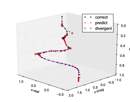
Figure 1: While tracking one solution path we show one coordinate of each solution point on the path. Corrected points (marked by a star) are connected as they lie on the path. Points that are not connected are predicted points (marked by a dot). Points from where the corrector diverged are marked by a circle.

Before we apply Newton’s method as a corrector, a predictor extrapolates the current solution ${\bf x}$ at the current value for $t$ to the next point on the path. Based on the outcome of the convergence of Newton’s method, an adaptive step size control strategy increases or decreases the step size $\Delta t$.

In one Newton step we compute $\Delta{\bf z}$ as the solution of

$$J_{\bf f}({\bf z})\Delta{\bf z}=-{\bf f}({\bf z}),$$ (2)

where $J_{\bf f}$ denotes the matrix of all partial derivatives of the system ${\bf f}({\bf x})={\bf 0}$. Then the current approximation is updated as ${\bf z}:={\bf z}+\Delta{\bf z}$. To continue with the next Newton step, we run the tests

$$\|{\bf f}({\bf z})\|\leq\epsilon_{\|{\bf f}({\bf z})\|}\quad{\rm and}\quad\|\Delta{\bf z}\|\leq\epsilon_{\|\Delta{\bf z}\|}$$ (3)

where $\|{\bf f}({\bf z})\|$ and $\|\Delta{\bf z}\|$ are respectively the backward and forward error of the problem.

Path following in an artificial-parameter homotopy follows an increment-and-fix strategy. The homotopy continuation parameter $t$ is increased independently of the coordinates of ${\bf x}$ in the predictor stage, as

$$t:=t+\Delta t,\quad{\rm with}\quad h_{\rm min}\leq\Delta t\leq h_{\rm max}.$$ (4)

Because the parameter $t$ in our homotopies (1) is artificial we apply the increment-and-fix predictor-corrector methods to solution paths in complex space. Our use of extended precision arithmetic is targeted to overcome the numerical instabilities that arise from working with higher degree polynomials which leads to matrices that may contain numbers of various magnitudes. In Table 8 we report several instances where one level of precision does not suffice to successfully track a solution path to the end.

Problem Statement. The difficulty to accelerate the tracking of one single path is that the predictor-corrector method is a strictly sequential process. Although we compute many points on a solution path, we cannot compute those points in parallel, independently from each other. In order to move to the next point on the path, the correction for the previous point must be completed. This difficulty requires a fine granularity in the parallel algorithm and a sufficiently high enough threshold on the dimension of the problem.

3 Accelerating Path Trackers

In this section we explain the implementation of path tracking with predictor-corrector methods in an increment-and-fix approach for artificial-parameter polynomial homotopies. We start with the high level descriptions and then go into the finer details of the accelerated algorithms.

3.1 Accelerated Predictor-Corrector

The input format for a polynomial system is a fully expanded distributed symbolic representation of a list of polynomials. This representation fits our choice of polynomial evaluation and differentiation algorithms. In the reverse mode of algorithmic differentiation, the focus is on a product of variables, which provides a large amount of thread parallelism, suitable for GPUs. Our path tracker computes with complex arithmetic in three modes: in double, double double, or quad double precision.

In the first stage, the value for the homotopy continuation parameter is incremented as $t:=t+\Delta t$ and the corresponding solution ${\bf x}$ is updated using extrapolation methods. Denoting $k$ as the degree of extrapolation polynomial, the values for $t$ as $t_{0}$, $t_{1}$, $\ldots$, $t_{k}$, and the corresponding coordinates as $x_{i}(t_{0})$, $x_{i}(t_{1})$, $\ldots$, $x_{i}(t_{k})$, then the predicted value for $x_{i}(t)$ at the new value for $t$ is obtained by evaluating a $k$th degree polynomial interpolating through those points. As the extrapolation occurs independently for each solution coordinate, as many threads as the dimension $n$ are occupied. But even with complex quad double arithmetic, the predictor stage has cost $O(n)$, significantly less than the other stages.

Figure 2 lists pseudocode for the accelerated corrector, illustrating the synchronizations performed by the kernel launches and the memory transfers from the device to the host to determine the convergence.

Input:	$Inst$, Polynomial Instructions
	$W$, GPU Workspace
	$P$, parameters for Newton’s method
Out	put	:	$success$ or $fail$
			updated $W.{\bf x}$
$last\_max\_eq\_val$ = $P.max\_eq\_val$
for $k$ from 1 to $P.max\_iteration$ do
	GPU_Eval($Inst$,$W$)
	laun	ch kernel Max_Array($W.eq\_val$, $max\_eq\_val$)
		with single block
	copy $max\_eq\_val$ from GPU to host
	if ($max\_eq\_val>last\_max\_eq\_val$)
		return $fail$
	if ($max\_eq\_val<P.tolerance$)
		return $success$
	GPU_Modified_Gram_Schmidt($W$)
	launch kernel Max_Array($W.\Delta{\bf x}$, $max\_\Delta{\bf x}$)
		with single block
	copy $max\_\Delta{\bf x}$ from GPU to host
	launch kernel Update_${\bf x}$($W.{\bf x}$,$W.\Delta{\bf x}$)
	if ($max\_\Delta{\bf x}<P.tolerance$)
		return $success$
	$last\_max\_eq\_val$ = $max\_eq\_val$
return $fail$

Figure 2: An accelerated Newton’s method.

The step control coincides with the launching of new kernels which can be done on the host, as only a constant amount of data (independent of the size of the problem) needs to be transferred between host and device. In particular, to determine the success of Newton’s method, the device computes a norm of the update $\|\Delta{\bf x}\|$, the norm the residual vector $\|{\bf f}({\bf x})\|$ and sends this number to the host. In reply, the device receives the new step size from the host before launching the next predictor-corrector kernel. As the host controls step size, there is a constant amount of data transfer from device to host. This size of these data does not depend on the size of the problem.

Keeping in mind the goal of minimizing the communication between host and device, we make the following arrangements. Transferring the polynomial structures, the coefficients, the start solution from the host to the device occurs only once at the start of the path tracking. In Newton’s method, $\|\Delta{\bf x}\|$ and $\|{\bf f}({\bf x})\|$ are used to control the Newton iteration, sent from device to host. The host uses these values to check whether the corrector converged or diverged and to determine whether to launch a new corrector kernel. The step size $\Delta t$ is controlled by the host. After each predictor-corrector stage, the host updates $t$ by $\Delta t$, and sends this update to the device. Then the predictor on the device uses the updated values to predict the next point on the path. When $t$ gets to $1$, the final solution ${\bf x}$ is sent from the device to the host.

The computation of the norm of the value of the solution at the system and the magnitude of the update to the solution can happen in ordinary double arithmetic as we are only concerned in the magnitude of the norms. With communications of these 3 double variables between host and device, then host can control the device to launch the kernels that run the path tracker.

Pseudocode for the path tracker is sketched in Figure 3. The GPU_Newton call refers to the algorithm in Figure 2. The decision to execute the step control at the host is motivated by its low computational cost and the desire to monitor the quality of the computations as the tracker advances along a solution path. Although the latest versions of CUDA allow for separate kernel launches initiated at the device, the fine granularity of our algorithms allows for the host to monitor the progress of the Newton steps.

Input:	$Inst$, Polynomial Instructions
	$W$, GPU Workspace
	$P$, parameters for path tracker
Out	put	:	$success$ or $fail$
			$W.{\bf x}$, solution for $t=1$ if $success$
$t=0$
$\Delta t=P.max\Delta t$
$\#successes=0$
$\#steps=0$
while $t<1$ do
	if ($\#steps>P.max\#steps$)
		return $fail$
	$t=\min(1,t+\Delta t$)
	copy $t$ from host to GPU
	launch kernel predict($W.{\bf x}\_array$, $W.t\_array$)
	$newton\_success$ = GPU_Newton($Inst$,$W$,$P$)
	if (	$newton\_success$)
		Update pointer of $W.{\bf x}$ in $W.{\bf x}\_array$
		$\#successes$ = $\#successes$ + 1
		if (	$\#successes>2$)
			$\Delta t=\min(2\Delta t,P.max\Delta t)$
	else
		$\#successes=0$
		$\Delta t=\Delta t/2$
	$\#steps=\#steps+1$
return $success$

Figure 3: Accelerated tracking of one single path.

3.2 Monomial Evaluation and Differentiation

We can evaluate and differentiate a single product of variables (the so-called example of Speelpenning) in two ways: in the reverse mode or with an arithmetic circuit, organized in a binary tree (as we described in [43]). The latter circuit can use several threads or even occupy an entire block to evaluate a single monomial, whereas the straightforward application of the reverse mode has to be executed by a single thread. If $n$ denotes the number of variables in a product, then the reverse mode writes about $n$ values to global memory to store intermediate results, whereas the reorganization in a binary tree keeps intermediate results in shared memory. The drawback however is that the binary tree structure of the algorithm limits the number of threads that can be used at each level of the tree. The organization in a binary tree is better for memory bound computations, which is the case when we work in double precision. But for compute bound computations, as is the case with double double and quad double arithmetic, the reverse mode is better.

To balance the work loads for each block, we sort the products of the variables according to the number of variables that appear in the product, so all threads in a single block work on products of similar size. For improved access to global memory, the data structures are designed to allow for coalesced reading and writing. The instructions to evaluate a product include the number of variables that occur in the product and the positions to indicate where each variable occurs in the product. Aligning numbers of variables and indices to positions, all threads are reading from global memory from consecutive locations at the same step. Access to global memory for intermediate and final results is handled in the same way. Table 1 illustrates the evaluation and differentiation of a product of variables.

Figure 4 illustrates the comparison of the original reverse mode, reverse mode with aligned memory and the tree mode in complex double precision. The polynomial system in this experiment is defined in (10). After alignment, the reverse mode improves, especially for larger dimension systems. The tree mode still works better for complex double precision. But for larger monomials, due to the limits of threads in the tree mode, reverse mode with aligned memory almost catches up. This new reverse mode also works better for double double and quad double arithmetic.

tidx	0	1	2	3
$m_{tidx}$	$x_{0}x_{1}x_{2}$	$x_{3}x_{4}x_{5}$	$x_{2}x_{3}x_{4}x_{5}$	$x_{0}x_{1}x_{3}x_{4}x_{5}$
$\displaystyle\frac{\partial m_{tidx}}{\partial x_{j}}$
	$x_{0}$	$x_{3}$	$x_{2}$	$x_{1}$
	$x_{0}\star x_{1}$	$x_{3}\star x_{4}$	$x_{2}\star x_{3}$	$x_{1}\star x_{2}$
			$x_{2}x_{3}\star x_{4}$	$x_{1}x_{2}\star x_{3}$
				$x_{1}x_{2}x_{3}\star x_{4}$
the forward calculation, from the top to bottom row

tidx	0	1	2	3
$m_{tidx}$	$x_{0}x_{1}x_{2}$	$x_{3}x_{4}x_{5}$	$x_{2}x_{3}x_{4}x_{5}$	$x_{0}x_{1}x_{3}x_{4}x_{5}$
$\displaystyle\frac{\partial m_{tidx}}{\partial x_{j}}$	$x_{1}\star x_{2}$	$x_{3}\star x_{4}x_{5}$	$x_{3}\star x_{4}x_{5}$	$x_{2}\star x_{3}x_{4}x_{5}$
	$x_{0}\star x_{2}$	$x_{3}\star x_{5}$	$x_{2}\star(x_{4}\star x_{5})$	$x_{1}\star(x_{3}\star x_{4}x_{5})$
	$x_{0}x_{1}$	$x_{3}x_{4}$	$x_{2}x_{3}\star x_{5}$	$x_{1}x_{2}\star(x_{4}\star x_{5})$
			$x_{2}x_{3}x_{4}$	$x_{1}x_{2}x_{3}\star(x_{5})$
				$x_{1}x_{2}x_{3}x_{4}$
backward and cross products, from bottom to top row

Table 1: Evaluating four monomials $x_{0}x_{1}x_{2}$, $x_{3}x_{4}x_{5}$, $x_{2}x_{3}x_{4}x_{5}$, $x_{0}x_{1}x_{3}x_{4}x_{5}$. The tidx in the tables below stands for thread index.

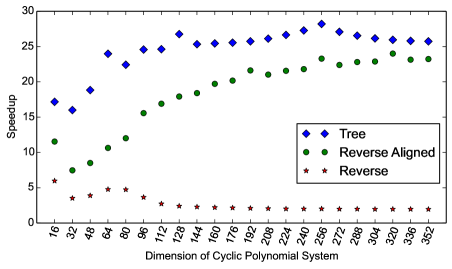
Figure 4: Monomial evaluation and differentiation speedup comparison in complex double precision

3.3 Number of Threads in the Summation

We improved the efficiency of our summation routines over those in [43]. We reorganized the summation algorithm so many threads work on one sum. This led to an increased amount of parallelism and an improved coalesced access to the main memory of the device. Even already in double precision arithmetic, double digits speedups of the accelerated code were obtained.

Tables 2 and 3 illustrate that the best speedups are obtained if four threads are collaborating to perform the summation. Working with a finer granularity increase the parallelism, but also leads to a larger number of blocks. Observe that on the GPU all times in the quad double column are all less than the time on the CPU. With acceleration, we can quadruple the precision and still be about twice faster than without acceleration. The polynomial system in this experiment is defined in (10).

	#Th	D	S	DD	S	QD	S
CPU		3.86		21.67		136.64
GPU	1	0.65	5.90	1.26	17.22	1.89	72.29
	2	0.44	8.85	0.56	38.57	1.38	99.18
	4	0.34	11.35	0.53	41.21	1.35	100.90
	8	0.37	10.53	0.63	34.39	1.54	88.44
	16	0.45	8.56	0.86	25.29	1.97	69.20
	32	0.65	5.89	0.96	22.59	2.58	53.00

Table 2: Summation times in milliseconds for cyclic 128-roots with an increasing number of threads ${\tt\#Th}$ per monomial on the GPU, for complex arithmetic in double (${\tt D}$), double double (${\tt DD}$), and quad double precision (${\tt QD}$), with Speedup (${\tt S}$) relative to one CPU core.

	#Th	D	S	DD	S	QD	S
CPU		95.02		422.71		2512.66
GPU	1	13.10	7.25	20.23	20.90	32.36	77.64
	2	7.50	12.66	9.97	42.41	24.61	102.10
	4	6.32	15.04	9.69	43.63	24.65	101.92
	8	6.91	13.75	11.24	37.61	27.60	91.03
	16	8.37	11.36	15.06	28.06	33.36	75.32
	32	12.37	7.68	16.35	25.86	39.37	63.82

Table 3: Summation times in milliseconds for cyclic 352-roots with an increasing number of threads ${\tt\#Th}$ per monomial on the GPU, for complex arithmetic in double (${\tt D}$), double double (${\tt DD}$), and quad double precision (${\tt QD}$). with Speedup (${\tt S}$) relative to one CPU core.

	#Th	D	S	DD	S	QD	S
CPU		196.90		918.25		3145.17
GPU	1	77.61	2.54	152.48	6.02	241.87	13.00
	2	29.43	6.69	46.45	19.77	124.68	25.23
	4	18.19	10.83	27.09	33.89	71.72	43.86
	8	14.16	13.90	18.96	48.44	46.51	67.63
	16	12.76	15.43	15.30	60.02	35.20	89.34
	32	14.58	13.50	14.46	63.52	30.53	103.02

Table 4: Summation times in milliseconds for the Pieri problem of dimension 103 with an increasing number of threads #Th per monomial on the GPU, for complex arithmetic in double (D), double double (DD), and quad double precision (QD). with Speedup (S) relative to one CPU core.

Table 4 displays timings to evaluate and differentiation a polynomial system arising from the minor expansions, as in (5). Increasing the number of collaborating threads keeps increasing the speedup. Except for the case when only one thread works on one monomial, the speedup is sufficiently large for the overhead caused by quadrupling the precision.

4 Test Problems

We chose two classes of benchmark polynomial systems that can be formulated for any dimension. In the first problem, we bootstrap from a linear system into a gradually higher dimensional and higher degree problem. Monodromy is applied in the second benchmark problem and the homotopies connect polynomial systems of the same complexity.

4.1 Matrix Completion with Pieri Homotopies

Our first class of test problems has its origin in the output pole placement problem in the control of linear systems. We may view this problem as an inverse eigenvalue problem [24]. The polynomial equations arise from minor expansions on

$$\det(A|X)=0,\quad A\in\mathbb{C}^{n\times m},$$ (5)

and where $X$ is an $n$-by-$p$ matrix ($m+p=n$) of unknowns. For example, a 2-plane in complex 4-space (or equivalently, a line in projective 3-space) is represented as

$$X=\left[\begin{array}[]{cc}1&0\\ x_{2,1}&1\\ x_{2,2}&x_{3,2}\\ 0&x_{4,2}\\ \end{array}\right].$$ (6)

To determine for the four unknowns in $X$ we need four equations as in (5), which via expansion results in four quadratic equations. In the application of Pieri homotopy algorithm (see e.g. [22], [23], [28], and [35]), we consider matrices $X$:

$$\left[\begin{array}[]{cc}1&0\\ 0&1\\ 0&x_{3,2}\\ 0&0\\ \end{array}\right],\quad\left[\begin{array}[]{cc}1&0\\ 0&1\\ 0&x_{3,2}\\ 0&x_{4,2}\\ \end{array}\right],\quad\left[\begin{array}[]{cc}1&0\\ x_{2,1}&1\\ 0&x_{3,2}\\ 0&x_{4,2}\\ \end{array}\right],$$ (7)

and then ends in the matrix X of (6). Each matrix in the sequence introduces one new variable and the homotopy starts at a solution of the previous homotopy, extended with a zero value for the new variable, each time a new matrix $A$ is introduced.

Using a superscript to index a sequence of matrices, $A^{(i)}\in\mathbb{C}^{n\times m}$, $i=1,2,\ldots,k$, Pieri homotopies are defined as

$${\bf h}({\bf x},t)=\left\{\begin{array}[]{l}\det(A^{(i)}|X)=0,~{}i=1,2,\ldots,k-1,\\ \det(tA^{(k)}+(1-t)S_{X}|X)=0,\end{array}\right.$$ (8)

where $S_{X}$ is a special matrix which ensures that for $t=0$, we have start solutions by setting the bottommost variables of $X$ to zero. Because of the similarities in the monomial structure, for this fully determined type of Pieri homotopy we may consider as last equation in the homotopy

$$t\det(A^{(k)}|X)+(1-t)\det(S_{X}|X)=0.$$ (9)

In the sequence of homotopies, the index $k$ runs from 1 to $m\times p$. Because in our setup, we track one single path, we may start at $k=m-1$, which corresponds to a linear system as only the last column of $X$ contains variables. As $k$ increases, the polynomial homotopy becomes more and more nonlinear. In the last stages of the homotopy, for $p=3$, the cost of evaluation via the minor expansions becomes cubic in $n$. As the cost of evaluation and differentiation becomes dominant, the most important factor lies in the summation of the many terms in every polynomial.

4.2 Monodromy on Cyclic $n$-roots

Our second test problem is the cyclic $n$-roots problem, denoted by ${\bf f}({\bf x})={\bf 0}$, ${\bf f}=(f_{1},f_{2},\ldots,f_{n})$, with

$$\begin{array}[]{l}f_{1}=x_{0}+x_{1}+\cdots+x_{n-1},\\ f_{2}=x_{0}x_{1}+x_{1}x_{2}+\dots+x_{n-2}x_{n-1}+x_{n-1}x_{0},\\ f_{i}=\displaystyle\sum_{j=0}^{n-1}~{}\prod_{k=j}^{j+i-1}x_{k~{}{\rm mod}~{}n},i=3,4,\ldots,n-1,\\ f_{n}=x_{0}x_{1}x_{2}\cdots x_{n-1}-1.\\ \end{array}$$ (10)

Observe the increase of the degrees: $\deg(f_{k})=k$. This implies that evaluating the system at points with coordinates of modulus different from one has the potential to lead to either very small or to very large numbers.

(a) Path 1

(b) Path 2

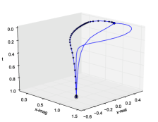
(c) Path 3

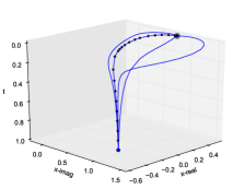
(d) Path 4

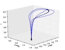
(e) Path 5

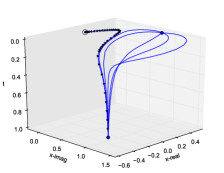
(f) Path 6

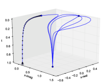
(g) Path 7

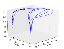
(h) Path 8

Figure 5: Visualization of monodromy on cyclic 4-roots, which has two solution sets of degree 2. Each subfigure adds a new path. Corrected points on path are marked by a star and the target point is circled.

Backelin’s Lemma [4] states that this system has a solution set of dimension $m-1$ for $n=\ell m^{2}$, where $\ell$ is no multiple of $k^{2}$, for $k\geq 2$. The system benchmarks polynomial solvers, see e.g. [14], [15], and [32]. In [2] we derived an explicit parameter representation for those positive dimensional cyclic $n$-roots solution sets. To compute the degree of the sets, we add as many linear equations $\bf L$ (with random complex coefficients) as the dimension of the set and count the number of solutions of the system ${\bf f}({\bf x})={\bf 0}$, augmented with $\bf L$:

$$\left\{\begin{array}[]{l}{\bf f}({\bf x})={\bf 0}\\ {\bf L}({\bf x})={\bf 0}.\end{array}\right.$$ (11)

The explicit representation of the cyclic $n$-roots solution sets allows for a quick calculation of the degrees, displayed in Table 5. From [1, Proposition 4.2], we have that the degree $d=m$ for $n=m^{2}$ and this result extends for $n=\ell m^{2}$.

$n$	16	32	48	64	80	96	128	144	160	176
$d$	4	4	4	8	4	4	8	12	4	4
$n$	192	208	240	256	272	288	304	320	336	352
$d$	8	4	4	16	4	12	4	8	4	4

Table 5: Degrees $d$ of the cyclic $n$-roots solution sets.

Observe that many solution sets in Table 5 have degree four. A fourth-order predictor will give accurate predictions on a surface of degree four. Therefore, the numerically harder problems are those dimensions for which the degree of the solution set is larger than four. For cyclic 64-roots double precision is no longer sufficient.

As done in PHCpack [33], with monodromy, the degree is computed numerically, using a sequence of homotopies:

$${\bf h}_{\alpha}({\bf x},t) = \left\{\begin{array}[]{c}{\bf f}({\bf x})={\bf 0}\\ \alpha(1-t){\bf L}({\bf x})+t{\bf K}({\bf x})={\bf 0}\end{array}\right.$$ (14)

$${\bf h}_{\beta}({\bf x},t) = \left\{\begin{array}[]{c}{\bf f}({\bf x})={\bf 0}\\ \beta(1-t){\bf K}({\bf x})+t{\bf L}({\bf x})={\bf 0}\end{array}\right.$$ (17)

where ${\bf K}({\bf x})={\bf 0}$ is as ${\bf L}({\bf x})={\bf 0}$ another set of linear equations with random coefficients and where $\alpha$ and $\beta$ are different random complex constants. One loop consists in tracking one path defined by ${\bf h}_{\alpha}({\bf x},t)={\bf 0}$ and ${\bf h}_{\beta}({\bf x},t)={\bf 0}$. In both cases $t$ goes from 0 to 1. See Figure 5.

After sufficiently many loops, each time for different values of the random constants $\alpha$ and $\beta$, we will find as many different solutions of the system (11) as the degree of the solution set, as in Table 5.

5 Computational Results

In this section we report timings and speedups.

5.1 Hardware and Software Environments

We implemented the path tracker with the gcc compiler and version 6.5 of the CUDA Toolkit. Our NVIDIA Tesla K20C, which has 2496 cores with a clock speed of 706 MHz, is hosted by a Red Hat Enterprise Linux workstation of Microway, with Intel Xeon E5-2670 processors at 2.6 GHz. Our code is compiled with the optimization flag -O2.

The code is at https://github.com/yxc2015/Path. The benchmark data were prepared with phcpy [38], the Python interface to PHCpack, in particular, with the scripts backelin.py and pierisystems.py of the examples directory of the PHCpy package.

5.2 Running Pieri Homotopies

Tables 6 and 7 summarize the execution of a sequence of Pieri homotopies, for dimensions $n$ ranging from 32 and 96. For each path, we list the number $m$ of predictor-corrector stages, which is the same for the host and device, as we use the same step length control strategy for both.

Note that timings in Tables 6 and 7 are rounded. The speedups are computed on the original timings.

$n$	$m$	cpu	gpu	S	$n$	$m$	cpu	gpu	S
32	25	0.05	0.05	1.1	65	63	5.6	0.7	8.0
33	150	0.70	0.55	1.3	66	187	25.3	2.4	10.7
34	65	0.44	0.30	1.5	67	98	17.4	1.3	13.1
35	101	0.84	0.49	1.7	68	239	50.0	3.2	15.8
36	36	0.40	0.21	1.9	69	244	68.0	3.7	18.4
37	10	0.13	0.06	2.1	70	118	40.4	2.0	20.1
38	37	0.56	0.25	2.3	71	41	17.0	0.8	21.9
39	24	0.44	0.18	2.4	72	89	41.8	1.8	23.2
40	19	0.39	0.15	2.6	73	99	44.2	1.8	24.6
41	52	1.12	0.41	2.7	74	85	41.9	1.7	25.0
42	66	1.38	0.48	2.9	75	89	50.3	1.9	26.0
43	72	1.67	0.55	3.0	76	246	136.0	4.6	29.8
44	23	0.61	0.19	3.2	77	100	53.3	1.9	27.7
45	16	0.45	0.13	3.4	78	81	45.7	1.6	28.2
46	25	0.74	0.21	3.5	79	272	210.0	6.2	34.0
47	27	0.90	0.24	3.7	80	226	158.0	5.5	28.7
48	53	1.69	0.45	3.8	81	50	39.0	1.3	29.4
49	32	1.05	0.27	3.9	82	116	91.2	3.1	29.1
50	108	3.77	0.94	4.0	83	136	107.2	3.6	29.5
51	48	1.67	0.41	4.1	84	69	59.2	2.0	29.6
52	79	2.97	0.71	4.2	85	248	206.5	6.9	30.1
53	53	2.06	0.47	4.4	86	181	166.5	5.3	31.2
54	91	3.37	0.75	4.5	87	32	31.1	1.0	30.5
55	18	0.90	0.19	4.6	88	36	37.3	1.2	30.2
56	28	1.37	0.29	4.7	89	94	113.7	3.2	36.0
57	45	2.01	0.42	4.7	90	73	75.7	2.5	29.9
58	34	1.69	0.35	4.8	91	66	68.4	2.3	30.1
59	29	1.41	0.28	5.0	92	90	98.0	3.2	30.3
60	111	5.70	1.13	5.1	93	102	112.6	3.7	30.3
61	67	3.77	0.74	5.1	94	41	40.2	1.3	30.4
62	42	2.40	0.46	5.3	95	53	61.4	1.8	34.4
63	85	4.85	0.91	5.3	96	64	67.2	2.2	30.8
64	63	3.36	0.62	5.4

Table 6: Running the first instance of Pieri homotopies in complex double double arithmetic, from dimensions 32 to 96. The units of the times on CPU and GPU are seconds. The last column for each dimension contains the speedup S.

$n$	$m$	cpu	gpu	S	$n$	$m$	cpu	gpu	S
32	16	0.03	0.03	1.1	68	51	11.3	0.7	15.6
33	68	0.38	0.30	1.3	69	60	17.9	1.0	18.2
34	21	0.16	0.10	1.5	70	22	7.7	0.4	21.1
35	19	0.20	0.11	1.7	71	156	62.0	2.8	22.1
36	18	0.20	0.11	1.9	72	39	19.4	0.8	23.4
37	34	0.44	0.21	2.1	73	49	26.9	1.1	24.2
38	32	0.44	0.19	2.3	74	98	56.7	2.3	24.6
39	41	0.65	0.26	2.5	75	74	43.6	1.7	25.9
40	12	0.25	0.09	2.6	76	63	38.8	1.5	26.4
41	17	0.36	0.13	2.9	77	37	27.1	1.0	27.0
42	29	0.65	0.23	2.9	78	95	67.9	2.5	27.6
43	66	1.47	0.48	3.1	79	112	76.6	2.8	27.7
44	10	0.28	0.08	3.2	80	157	115.0	4.0	28.8
45	46	1.30	0.39	3.4	81	321	265.2	7.6	35.0
46	31	0.85	0.24	3.5	82	63	47.9	1.6	29.6
47	51	1.60	0.44	3.6	83	42	33.3	1.1	29.9
48	16	0.54	0.14	3.8	84	19	17.3	0.6	30.0
49	16	0.58	0.15	3.9	85	224	188.1	6.2	30.2
50	24	0.91	0.23	3.9	86	159	147.9	4.3	34.1
51	62	2.31	0.56	4.1	87	252	199.4	6.4	31.0
52	40	1.52	0.36	4.3	88	574	431.2	13.3	32.4
53	46	2.09	0.49	4.2	89	213	171.3	5.5	30.9
54	33	1.62	0.37	4.4	90	137	129.9	3.6	35.9
55	79	3.84	0.86	4.5	91	187	157.8	5.0	31.7
56	36	1.71	0.36	4.7	92	250	219.8	6.1	36.2
57	42	2.23	0.48	4.6	93	847	646.1	19.3	33.4
58	29	1.58	0.33	4.8	94	199	169.1	4.9	34.6
59	37	1.98	0.40	4.9	95	108	96.1	3.1	31.0
60	16	0.95	0.19	5.0	96	190	230.8	6.2	37.1
61	37	2.10	0.41	5.2	97	161	305.3	6.7	45.8
62	50	2.97	0.57	5.2	98	76	264.7	4.4	60.5
63	34	1.95	0.36	5.4	99	75	322.6	5.5	58.7
64	75	4.54	0.84	5.4	100	242	1367.2	23.0	59.4
65	83	7.93	0.96	8.3	101	809	4655.7	70.7	65.9
66	195	27.20	2.56	10.6	102	1016	5231.7	75.6	69.2
67	154	26.43	2.07	12.8	103	375	2923.2	44.0	66.5

Table 7: Running the second instance of Pieri homotopies in complex double double arithmetic, from dimensions 32 to 103. The units of the times on CPU and GPU are seconds. The last column for each dimension contains the speedup S.

Tables 6 and 7 are visualized in Figures 6 and 7. Because the fluctuations in the number of predictor-corrector steps along a path can vary by a factor as large as five, the single digit speedups obtained by acceleration in low dimensions is often in the same range as the factor in the fluctuations of the timings. While fluctuations in larger dimensions remain of the same order, the double digit speedups make that with acceleration we may increase the dimension, compare for example the lines for $n=63$ and $n=96$ in Table 6 and still be faster: 2.2 seconds versus 4.85 seconds.

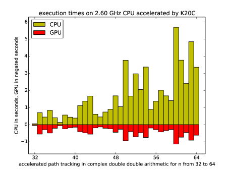
Figure 6: Visualization of the first half of Table 6. While the times on the GPU are always smaller than the CPU times for the same dimension, fluctuations in the number of steps, e.g.: compare $n=59$ with $n=60$ may matter more.

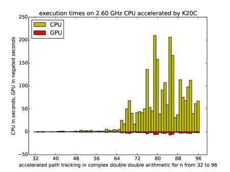
Figure 7: Visualization of the entire Table 6. With a more than double speedup of the GPU over the CPU, fluctuations in times caused by a variable number of steps no longer matter.

Double digit speedups arise after dimension 65. After dimension 97, the speedup then almost doubles, see Figure 8.

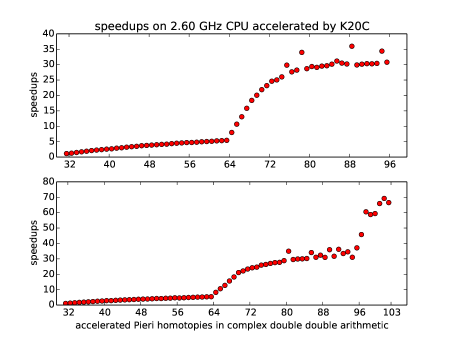
Figure 8: Visualization of the speedups of Table 6 on top, with speedups of Table 7 below. Observe the different ranges of the vertical axes.

5.3 Running One Path of Cyclic $n$-roots

Table 8 summarizes the computational results from running one path on a homotopy to apply the monodromy on the cyclic $n$-roots problem. The first case where double precision does not suffice is in dimension $n=64$, but the path can then be tracked successfully in double double precision. For $n=144$, both double and double double precision are insufficient and quad double precision is needed.

The difficulties could be explained by the higher degree of the solution set. Cyclic 256-roots remains a challenge. The double digit speedups obtained by acceleration implies that we can offset the cost of one extra level of higher precision.

	complex double					complex double double					complex quad double
$n$	$s$	$m$	cpu	gpu	S	$s$	$m$	cpu	gpu	S	$s$	$m$	cpu	gpu	S
16	1	32	0.00	0.03	0.14	1	20	0.04	0.06	0.65	1	32	0.48	0.52	0.92
32	1	100	0.06	0.16	0.35	1	79	1.03	0.41	2.53	1	100	12.66	3.62	3.50
48	1	103	0.17	0.24	0.72	1	78	3.23	0.61	5.29	1	103	39.46	5.39	7.32
64	0	987	4.48	4.15	1.08	1	225	22.94	2.57	8.92	1	987	229.99	17.93	12.83
80	1	99	0.73	0.42	1.74	1	75	14.96	1.15	13.01	1	99	180.37	10.13	17.81
96	1	95	1.23	0.52	2.36	1	69	23.17	1.34	17.26	1	95	289.38	12.64	22.90
112	1	171	3.42	1.17	2.92	1	121	68.07	2.98	22.86	1	171	813.91	28.36	28.70
128	1	162	5.66	1.47	3.85	1	123	102.94	3.88	26.54	1	162	1253.82	37.75	33.21
144	0	214	12.58	2.67	4.72	0	1500	1487.86	61.59	24.16	1	214	15898.67	479.18	33.18
160	1	68	4.84	0.87	5.53	1	49	83.11	2.84	29.31	1	68	998.43	23.96	41.67
176	1	160	15.65	2.52	6.21	1	118	259.80	8.06	32.24	1	160	3179.81	70.58	45.05
192	0	246	30.92	9.27	3.34	1	150	419.16	13.03	32.16	1	246	5054.70	105.69	47.83
208	1	231	39.51	5.22	7.57	1	168	628.46	16.33	38.48	1	231	7529.02	147.09	51.19
224	1	96	19.39	2.46	7.88	1	71	319.27	7.88	40.54	1	96	3925.33	73.76	53.22
240	1	140	34.04	4.04	8.42	1	96	531.01	12.49	42.50	1	140	6714.01	119.86	56.01
256	0	0	0.00	1.00	0.00	0	0	0.00	1.00	0.00	0	0	0.00	1.00	0.00
272	1	160	58.19	7.19	8.09	1	118	914.24	19.12	47.82	1	160	10829.36	183.12	59.14
288	0	0	0.00	1.00	0.00	0	0	0.00	1.00	0.00	0	0	0.00	1.00	0.00
304	1	142	81.04	8.05	10.07	1	103	1176.29	22.87	51.44	1	142	13992.60	226.78	61.70
320	0	0	0.00	1.00	0.00	0	0	0.00	1.00	0.00	0	0	0.00	1.00	0.00
336	1	157	105.30	11.12	9.47	1	114	1772.97	33.26	53.31	1	157	20807.27	327.25	63.58
352	1	121	93.89	9.78	9.60	1	90	1621.15	28.75	56.39	1	121	18881.13	290.36	65.03

Table 8: Running one path of cyclic $n$-roots in various precisions and in various dimensions. Data in the column under the header $s$ indicates success by ${\rm 1}$ or failure by ${\rm 0}$. The number of predictor-corrector steps equals $m$. The units of the times on CPU and GPU are seconds. The last column for each dimension and precision contains the speedup S.

The data in Table 8 for complex double and complex double double precision is visualized in Figure 9.

Concerning the data in Table 8, let us compare the accelerated times in double double precision to the times on one CPU core in double precision. For the last line, observe that it takes 93.89 seconds to track one path in double precision without acceleration. With acceleration tracking one path in double double precision takes 28.75 seconds, so we can double the precision and still be three times faster than in double precision without acceleration. Speedups computed in Table 8 are shown in Figure 9. We see that in double double precision, the speedups rise faster as the dimension increases than in double precision.

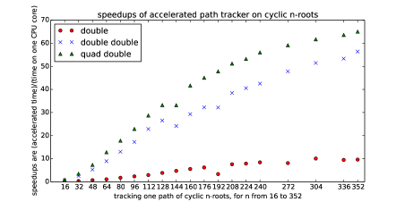
Figure 9: Visualization of the speedups of Table 8. In double precision, the dimensions are too small to achieve double digit speedups, but then also the precision may be insufficient. In double double precision, speedups are good as soon as the dimension reaches one hundred and they improved even further in quad double precision.

6 Concluding Remarks

This paper provides a description for an accelerated path tracker for polynomial homotopies. On two classes of benchmark problems we illustrate that for sufficiently high dimensions with acceleration we can compensate for the extra cost of high precision arithmetic.

References

- [1] D. Adrovic and J. Verschelde. Computing Puiseux series for algebraic surfaces. In J. van der Hoeven and M. van Hoeij, editors, Proceedings of the 37th International Symposium on Symbolic and Algebraic Computation (ISSAC 2012), pages 20–27. ACM, 2012.
- [2] D. Adrovic and J. Verschelde. Polyhedral methods for space curves exploiting symmetry applied to the cyclic -roots problem. In V.P. Gerdt, W. Koepf, E.W. Mayr, and E.V. Vorozhtsov, editors, Proceedings of CASC 2013, pages 10–29, 2013.
- [3] D. C. S. Allison, A. Chakraborty, and L. T. Watson. Granularity issues for solving polynomial systems via globally convergent algorithms on a hypercube. J. of Supercomputing, 3(1):5–20, 1989.
- [4] J. Backelin. Square multiples n give infinitely many cyclic n-roots. Reports, Matematiska Institutionen 8, Stockholms universitet, 1989.
- [5] T. Bartkewitz and T. Güneysu. Full lattice basis reduction on graphics cards. In F. Armknecht and S. Lucks, editors, WEWoRC’11 Proceedings of the 4th Western European conference on Research in Cryptology, volume 7242 of Lecture Notes in Computer Science, pages 30–44. Springer-Verlag, 2012.
- [6] D. J. Bates, J. D. Hauenstein, A. J. Sommese, and C. W. Wampler. Bertini: Software for numerical algebraic geometry. Available at http://www.nd.edu/sommese/bertini/.
- [7] W. Bauer and V. Strassen. The complexity of partial derivatives. Theoretical Computer Science, 22(3):317–330, 1983.
- [8] C. Bischof, N. Guertler, A. Kowartz, and A. Walther. Parallel reverse mode automatic differentiation for OpenMP programs with ADOL-C. In C. Bischof, H.M. Bücker, P. Hovland, U. Naumann, and J. Utke, editors, Advances in Automatic Differentiation, pages 163–173. Springer-Verlag, 2008.
- [9] N. Bliss, J. Sommars, J. Verschelde, and X. Yu. Solving polynomial systems in the cloud with polynomial homotopy continuation. arXiv:1506.02618 [cs.MS], accepted for publication in the Proceedings of the 17th Workshop on Computer Algebra in Scientific Computing (CASC 2015).
- [10] R. W. Brockett and C. I. Byrnes. Multivariate Nyquist criteria, root loci, and pole placement: a geometric viewpoint. IEEE Trans. Automat. Contr., 26:271–284, 1981.
- [11] T. Chen, T.-L. Lee, and T.-Y. Li. Hom4PS-3: a parallel numerical solver for systems of polynomial equations based on polyhedral homotopy continuation methods. In H. Hong and C. Yap, editors, Mathematical Software – ICMS 2014, 4th International Conference, Seoul, South Korea, August 4-9, 2014, Proceedings, volume 8592 of Lecture Notes in Computer Science, pages 183–190. Springer-Verlag, 2014.
- [12] T. Chen and T.-Y. Li. Solutions to systems of binomial equations. Annales Mathematicae Silesianae, 28:7–34, 2014.
- [13] T. Chen and D. Mehta. Parallel degree computation for solution space of binomial systems with an application to the master space of gauge theories. arXiv:1501.02237v1 [math.AG].
- [14] Y. Dai, S. Kim, and M. Kojima. Computing all nonsingular solutions of cyclic-n polynomial using polyhedral homotopy continuation methods. J. Comput. Appl. Math., 152(1-2):83–97, 2003.
- [15] J. C. Faugère. Finding all the solutions of Cyclic 9 using Gröbner basis techniques. In Computer Mathematics - Proceedings of the Fifth Asian Symposium (ASCM 2001), volume 9 of Lecture Notes Series on Computing, pages 1–12. World Scientific, 2001.
- [16] T. Gao, T.-Y. Li, and X. Li. HOM4PS, 2002. Available at http://www.csulb.edu/tgao/ RESEARCH/Software.htm.
- [17] M. Grabner, T. Pock, T. Gross, and B. Kainz. Automatic differentiation for GPU-accelerated 2D/3D registration. In C. Bischof, H.M. Bücker, P. Hovland, U. Naumann, and J. Utke, editors, Advances in Automatic Differentiation, pages 259–269. Springer-Verlag, 2008.
- [18] A. Griewank and A. Walther. Evaluating Derivatives: Principles and Techniques of Algorithmic Differentiation. SIAM, second edition, 2008.
- [19] T. Gunji, S. Kim, M. Kojima, A. Takeda, K. Fujisawa, and T. Mizutani. PHoM – a polyhedral homotopy continuation method for polynomial systems. Computing, 73(4):55–77, 2004.
- [20] S. A. Haque, X. Li, F. Mansouri, M. M. Maza, W. Pan, and N. Xie. Dense arithmetic over finite fields with the CUMODP library. In H. Hong and C. Yap, editors, Mathematical Software – ICMS 2014, volume 8592 of Lecture Notes in Computer Science, pages 725–732. Springer-Verlag, 2014.
- [21] Y. Hida, X. S. Li, and D. H. Bailey. Algorithms for quad-double precision floating point arithmetic. In 15th IEEE Symposium on Computer Arithmetic (Arith-15 2001), 11-17 June 2001, Vail, CO, USA, pages 155–162. IEEE Computer Society, 2001. Shortened version of Technical Report LBNL-46996, software at http://crd.lbl.gov/dhbailey/ mpdist.
- [22] B. Huber, F. Sottile, and B. Sturmfels. Numerical Schubert calculus. J. Symbolic Computation, 26(6):767–788, 1998.
- [23] B. Huber and J. Verschelde. Pieri homotopies for problems in enumerative geometry applied to pole placement in linear systems control. SIAM J. Control Optim., 38(4):1265–1287, 2000.
- [24] M. Kim, J. Rosenthal, and X. Wang. Pole placement and matrix extension problems: A common point of view. SIAM J. Control. Optim., 42(6):2078–2093, 2004.
- [25] T. L. Lee, T.-Y. Li, and C. H. Tsai. HOM4PS-2.0: a software package for solving polynomial systems by the polyhedral homotopy continuation method. Computing, 83(2-3):109–133, 2008.
- [26] A. Leykin. Numerical algebraic geometry. The Journal of Software for Algebra and Geometry: Macaulay2, 3:5–10, 2011.
- [27] T.-Y. Li. Numerical solution of polynomial systems by homotopy continuation methods. In F. Cucker, editor, Handbook of Numerical Analysis. Volume XI. Special Volume: Foundations of Computational Mathematics, pages 209–304. North-Holland, 2003.
- [28] T.-Y. Li, X. Wang, and M. Wu. Numerical schubert calculus by the pieri homotopy algorithm. SIAM J. Numer. Anal., 20(2):578–600, 2002.
- [29] M. Lu, B. He, and Q. Luo. Supporting extended precision on graphics processors. In A. Ailamaki and P.A. Boncz, editors, Proceedings of the Sixth International Workshop on Data Management on New Hardware (DaMoN 2010), June 7, 2010, Indianapolis, Indiana, pages 19–26, 2010. Software at http://code.google.com/p/gpuprec/.
- [30] G. Malajovich. pss3.0.5: Polynomial system solver, version 3.0.5. Available at http://www.labma.ufrj.br/gregorio/software.php.
- [31] M. M. Maza and W. Pan. Solving bivariate polynomial systems on a GPU. ACM Communications in Computer Algebra, 45(2):127–128, 2011.
- [32] R. Sabeti. Numerical-symbolic exact irreducible decomposition of cyclic-12. LMS Journal of Computation and Mathematics, 14:155–172, 2011.
- [33] A. J. Sommese, J. Verschelde, and C. W. Wampler. Numerical irreducible decomposition using PHCpack. In M. Joswig and N. Takayama, editors, Algebra, Geometry, and Software Systems, pages 109–130. Springer-Verlag, 2003.
- [34] A.J. Sommese, J. Verschelde, and C.W. Wampler. Introduction to numerical algebraic geometry. In Solving Polynomial Equations. Foundations, Algorithms and Applications, volume 14 of Algorithms and Computation in Mathematics, pages 301–337. Springer-Verlag, 2005.
- [35] F. Sottile. Pieri’s formula via explicit rational equivalence. Can. J. Math., 49(6):1281–1298, 1997.
- [36] F. Szöllősi. Construction, classification and parametrization of complex Hadamard matrices. PhD thesis, Central European University, Budapest, 2011. arXiv:1110.5590v1.
- [37] J. Verschelde. Algorithm 795: PHCpack: A general-purpose solver for polynomial systems by homotopy continuation. ACM Trans. Math. Softw., 25(2):251–276, 1999.
- [38] J. Verschelde. Modernizing PHCpack through phcpy. In P. de Buyl and N. Varoquaux, editors, Proceedings of the 6th European Conference on Python in Science (EuroSciPy 2013), pages 71–76, 2014.
- [39] J. Verschelde and G. Yoffe. Polynomial homotopies on multicore workstations. In M.M. Maza and J.-L. Roch, editors, Proceedings of the 4th International Workshop on Parallel Symbolic Computation (PASCO 2010), July 21-23 2010, Grenoble, France, pages 131–140. ACM, 2010.
- [40] J. Verschelde and G. Yoffe. Evaluating polynomials in several variables and their derivatives on a GPU computing processor. In Proceedings of the 2012 IEEE 26th International Parallel and Distributed Processing Symposium Workshops (PDSEC 2012), pages 1391–1399. IEEE Computer Society, 2012.
- [41] J. Verschelde and G. Yoffe. Orthogonalization on a general purpose graphics processing unit with double double and quad double arithmetic. In Proceedings of the 2013 IEEE 27th International Parallel and Distributed Processing Symposium Workshops (PDSEC 2013), pages 1373–1380. IEEE Computer Society, 2013.
- [42] J. Verschelde and X. Yu. Tracking many solution paths of a polynomial homotopy on a graphics processing unit. arXiv:1505.00383v1, accepted for publication in the Proceedings of the 17th IEEE International Conference on High Performance Computing and Communications (HPCC 2015).
- [43] J. Verschelde and X. Yu. GPU acceleration of Newton’s method for large systems of polynomial equations in double double and quad double arithmetic. In Proceedings of the 16th IEEE International Conference on High Performance Computing and Communication (HPCC 2014), pages 161–164. IEEE Computer Society, 2014.
- [44] V. Volkov and J. Demmel. Benchmarking GPUs to tune dense linear algebra. In Proceedings of the 2008 ACM/IEEE conference on Supercomputing. IEEE Press, 2008. Article No. 31.
- [45] L. T. Watson, S. C. Billups, and A. P. Morgan. Algorithm 652: HOMPACK: a suite of codes for globally convergent homotopy algorithms. ACM Trans. Math. Softw., 13(3):281–310, 1987.
- [46] L. T. Watson, M. Sosonkina, R. C. Melville, A.P. Morgan, and H.F. Walker. HOMPACK90: A suite of Fortran 90 codes for globally convergent homotopy algorithms. ACM Trans. Math. Softw., 23(4):514–549, 1997.