Effects of Two Inert Scalar Doublets on Higgs Interactions and Electroweak Phase Transition

Abstract

We study some implications of the presence of two new scalar weak doublets beyond the standard model which have zero vacuum expectation values and are charged under an extra Abelian gauge symmetry. The additional gauge sector does not couple directly to standard-model particles. We investigate specifically the effects of the scalars on oblique electroweak parameters and on the interactions of the 125 GeV Higgs boson, especially its decay modes $h\rightarrow\gamma\gamma,\gamma Z$ and trilinear self-coupling, all of which will be probed with improved precision in future Higgs measurements. Moreover, we explore how the new scalars may give rise to strongly first-order electroweak phase transition and also show its correlation with sizable modifications to the Higgs trilinear self-coupling.

I Introduction

The recent discovery atlas:h ; cms:h at the Large Hadron Collider (LHC) of a Higgs boson with mass around 125 GeV and other properties consistent with the expectations of the standard model (SM) serves as yet another confirmation that it is a remarkably successful theory. Nevertheless, it is widely believed that new physics beyond it is still necessary at least to account for the compelling experimental evidence for neutrino mass and the astronomical indications of dark matter pdg .

Among a great many possibilities beyond the SM are those with enlarged scalar sectors. Scenarios incorporating a second Higgs doublet are of course highly popular in the literature thdm ; Branco:2011iw . Of late models with three scalar weak doublets have also been gaining interest Ivanov:2011ae ; Machado:2012ed ; Keus:2013hya ; Fortes:2014dia ; Maniatis:2014oza ; Ivanov:2014doa ; Moretti:2015cwa ; Keus:2014jha ; Ma:2013yga , as they can provide dark matter (DM) candidates Keus:2014jha and/or an important ingredient for the mechanism that generates neutrino mass Ma:2013yga .

Here we consider this three-scalar-doublet possibility, particularly that in which two of the doublets possess zero vacuum expectation values (VEVs). The theory also involves a new Abelian gauge symmetry under which these two doublets are charged, while SM particles are not. As a consequence, the extra scalar particles do not couple directly to a pair of exclusively SM fermions. Because of the absence of their VEVs and couplings to SM fermion pairs, these scalars have been termed inert in the literature Keus:2013hya . However, being members of weak doublets, these scalars have interactions with SM gauge bosons at tree level. In addition, the gauge boson associated with the new gauge group is taken to have vanishing kinetic mixing with the hypercharge gauge boson. Accordingly, the additional gauge sector can be regarded as dark.

With these choices, the scalar sector of the theory corresponds to one of the three-scalar-doublet models catalogued and studied in Ref. Keus:2013hya in terms of all possible allowed symmetries. In the present paper, we entertain the scenario described above and explore some implications of the presence of the inert scalars. Specifically, we analyze constraints on them from collider measurements on the Higgs boson and from electroweak precision data. In addition, we look at the potential impact of the scalars on the Higgs trilinear self-coupling, anticipating future experiments that will probe it sufficiently well. To evaluate the coupling, we will employ the Higgs effective potential derived at the one-loop level. Moreover, we examine how the new particles, which we choose to have sub-TeV masses, may give rise to strongly first-order electroweak phase transition (EWPT), which is needed for electroweak baryogenesis to explain the baryon asymmetry of the Universe. As it has been pointed out in the context of other models that the strength of EWPT could be correlated with sizable modifications to the Higgs trilinear self-coupling KOS ; Noble:2007kk ; Chiang:2014hia ; Fuyuto:2014yia ; Curtin:2014jma , our results will indicate how this may be realized in the presence of the new doublets.

Due to their tree-level interactions with SM gauge and Higgs bosons, the lightest of the inert scalars cannot serve as good candidates for DM, as they annihilate into SM particles too fast and hence cannot produce enough relic abundance. To account for DM, one needs to have a more complete theory, but we assume that the additional ingredients responsible for explaining DM have negligible or no impact on our scalar sector of interest, so that they do not affect the results of this paper.

The plan of the paper is as follows. In the next section, we describe the scalar Lagrangian and address some theoretical constraints on its parameters, especially from the requirements on vacuum stability. Since the extra scalar doublets couple to the standard Higgs and gauge bosons and include electrically-charged members, they contribute at the one-loop level to the Higgs decays  $h\rightarrow\gamma\gamma$  and  $h\rightarrow\gamma Z$  which have been under intense investigation at the LHC, the former channel having also been observed. We determine their rates in section III, where we also start our numerical analysis by exploring the charged scalars’ impact on these processes. In section IV, we calculate the contributions of the new doublets to the oblique electroweak observables $S$ and $T$, on which experimental information is available. Sections V and VI contain our treatment of the new scalars’ effects on the trilinear Higgs couplings and on the electroweak phase transition, respectively. After deriving the relevant formulas, we perform further numerical work in these sections. In section VII, we discuss additional results and make our conclusions after combining different relevant constraints. A few appendices contain more discussions and formulas.

II Scalar Sector

II.1 Lagrangian

Compared to the SM with the Higgs doublet $\Phi$, the scalar sector is expanded with the addition of two weak doublets, $\eta_{1}$ and $\eta_{2}$. The theory also possesses an extra Abelian gauge symmetry, $\mathrm{U(1)}{}_{D}$, under which $\eta_{1,2}$ carry charges $+1$ and $-1$, respectively, whereas SM particles are not charged. Accordingly, one can express the renormalizable Lagrangian for the interactions of the scalars with each other and with the standard $\mathrm{SU(2)}{}_{L}\times\mathrm{U(1)}{}_{Y}$ gauge bosons, $W_{1,2,3}$ and $B$, as well as the $\mathrm{U(1)}{}_{D}$ gauge boson $C$, as

$$\mathcal{L}=(\mathcal{D}^{\mu}\Phi)^{\dagger}\mathcal{D}_{\mu}\Phi+(\mathcal{D}^{\mu}\eta_{1})^{\dagger}\mathcal{D}_{\mu}\eta_{1}+(\mathcal{D}^{\mu}\eta_{2})^{\dagger}\mathcal{D}_{\mu}\eta_{2}\;-\;\mathcal{V},$$ (1)

where the covariant derivative  $\mathcal{D}^{\mu}=\partial^{\mu}+(ig/2)\tau_{j}W_{j}^{\mu}+ig_{Y}\mathcal{Q}_{Y}B^{\mu}+ig_{D}\mathcal{Q}_{C}C^{\mu}$  also contains the gauge couplings $g$, $g_{Y}$, and $g_{D}$, Pauli matrices $\tau_{1,2,3}$, and $\mathrm{U(1)}{}_{Y,D}$ charge operators $\mathcal{Q}_{Y,C}$, while the scalar potential is

$$\mathcal{V} =\mu_{1}^{2}\Phi^{\dagger}\Phi+\mu_{21}^{2}\eta_{1}^{\dagger}\eta_{1}+\mu_{22}^{2}\eta_{2}^{\dagger}\eta_{2}+\tfrac{1}{2}\lambda_{1}(\Phi^{\dagger}\Phi)^{2}+\tfrac{1}{2}\lambda_{21}(\eta_{1}^{\dagger}\eta_{1})^{2}+\tfrac{1}{2}\lambda_{22}(\eta_{2}^{\dagger}\eta_{2})^{2}$$

$$~{}~{}~{}+\lambda_{31}\Phi^{\dagger}\Phi\eta_{1}^{\dagger}\eta_{1}+\lambda_{32}\Phi^{\dagger}\Phi\eta_{2}^{\dagger}\eta_{2}+\lambda_{41}\Phi^{\dagger}\eta_{1}\eta_{1}^{\dagger}\Phi+\lambda_{42}\Phi^{\dagger}\eta_{2}\eta_{2}^{\dagger}\Phi$$

$$~{}~{}~{}+\tfrac{1}{2}\left[\lambda_{5}\Phi^{\dagger}\eta_{1}\Phi^{\dagger}\eta_{2}+\lambda_{5}^{\ast}\eta_{1}^{\dagger}\Phi\eta_{2}^{\dagger}\Phi\right]+\lambda_{6}\eta_{1}^{\dagger}\eta_{1}\eta_{2}^{\dagger}\eta_{2}+\lambda_{7}\eta_{1}^{\dagger}\eta_{2}\eta_{2}^{\dagger}\eta_{1}.$$ (2)

Thus  $\mathcal{Q}_{C}\Phi=0$  and  $\mathcal{Q}_{C}\eta_{1}(\eta_{2})=+\eta_{1}(-\eta_{2})$.  The parameters $\mu_{1,2a}^{2}$ and $\lambda_{1,2a,3a,4a,6,7}$ with  $a=1,2$  are necessarily real because of the hermiticity of $\mathcal{V}$, whereas $\lambda_{5}$ can be rendered real using the relative phase between $\Phi$ and $\eta_{1,2}$. Assuming that the $\mathrm{U(1)}{}_{D}$ symmetry stays intact, after electroweak symmetry breaking we can write

$$\Phi=\left(\begin{array}[c]{c}0\vspace{2pt}\\ \frac{1}{\sqrt{2}}(v+h)\end{array}\right),~{}~{}~{}~{}~{}~{}~{}\eta_{a}=\left(\begin{array}[c]{c}H_{a}^{+}\vspace{3pt}\\ \eta_{a}^{0}\end{array}\right),~{}~{}~{}~{}\sqrt{2}\;\eta_{a}^{0}=\mathrm{Re}\eta_{a}^{0}+i\mathrm{Im}\eta_{a}^{0}\;,$$ (3)

where $h$ represents the physical Higgs boson, $v\simeq 246$ GeV is the vacuum expectation value (VEV) of $\Phi$, and $H_{a}^{+}$ and $\eta_{a}^{0}$ denote, respectively, the electrically charged and neutral components of $\eta_{a}$, which has no VEV.

From the terms in $\mathcal{V}$ that are quadratic in the fields, it is straightforward to extract the mass eigenstates of the scalars. Thus the masses of $h$ and $H_{1,2}^{\pm}$ at tree level are given by

$$\hat{m}_{h}^{2}=\mu_{1}^{2}+\tfrac{3}{2}\lambda_{1}^{~{}}v^{2},~{}~{}~{}m_{H_{a}^{\pm}}^{2}=\mu_{2a}^{2}+\tfrac{1}{2}\lambda_{3a}v^{2}.$$ (4)

The $\lambda_{5}$ part in eq. (II.1) causes mixing between the electrically neutral components $\eta_{1}^{0}$ and $\eta_{2}^{0\ast}$, which are then related to the mass eigenstates $\chi_{1}$ and $\chi_{2}$ according to

$$\left(\!\begin{array}[c]{c}\eta_{1}^{0}\vspace{2pt}\\ \eta_{2}^{0\ast}\end{array}\!\right) =\left(\!\begin{array}[c]{ccc}c_{\theta}&&s_{\theta}\vspace{1pt}\\ -s_{\theta}&&c_{\theta}\end{array}\!\right)\left(\!\begin{array}[c]{c}\chi_{1}\vspace{1pt}\\ \chi_{2}\end{array}\!\right),~{}~{}~{}~{}~{}~{}~{}c_{\theta}=\cos\theta,~{}~{}~{}~{}s_{\theta}=\sin\theta,$$ (11)

$$\tan(2\theta) =\frac{\lambda_{5}v^{2}}{2m_{H_{2}^{\pm}}^{2}-2m_{H_{1}^{\pm}}^{2}+\left(\lambda_{42}-\lambda_{41}\right)v^{2}}\;,$$ (12)

the resulting eigenmasses being given by

$$m_{\chi_{1,2}}^{2} =\tfrac{1}{2}\left(m_{H_{1}^{\pm}}^{2}+m_{H_{2}^{\pm}}^{2}\right)+\tfrac{1}{4}\left(\lambda_{41}+\lambda_{42}\right)v^{2}$$

$$~{}~{}~{}\mp\tfrac{1}{2}\sqrt{\left[m_{H_{2}^{\pm}}^{2}-m_{H_{1}^{\pm}}^{2}+\tfrac{1}{2}\left(\lambda_{42}-\lambda_{41}\right)v^{2}\right]^{2}+\tfrac{1}{4}\lambda_{5}^{2}v^{4}}\;.$$ (13)

Hence the $\mathrm{U(1)}{}_{D}$ charges of $\chi_{1,2}$ are the same as (opposite in sign to) that of $\eta_{1}$ ($\eta_{2}$) and $m_{\chi_{1}}\leq m_{\chi_{2}}$.

Alternatively, instead of $\chi_{a}$, one can choose to deal with their real and imaginary parts,

$$\mathcal{S}_{a}=\sqrt{2}\;\mathrm{Re}\chi_{a},~{}~{}~{}~{}\mathcal{P}_{a}=\sqrt{2}\;\mathrm{Im}\chi_{a},$$ (14)

which are $CP$-even and $CP$-odd states, respectively, and share mass, $m_{\mathcal{S}_{a}}=m_{\mathcal{P}_{a}}=m_{\chi_{a}}$. From eq. (11), one then has in matrix form

$$\left(\begin{array}[c]{c}\mathrm{Re}\eta_{1}^{0}\\ \mathrm{Re}\eta_{2}^{0}\\ \mathrm{Im}\eta_{1}^{0}\\ \mathrm{Im}\eta_{2}^{0}\end{array}\right)=\left(\begin{array}[c]{ccccccc}c_{\theta}&&s_{\theta}&&0&&0\\ -s_{\theta}&&c_{\theta}&&0&&0\\ 0&&0&&c_{\theta}&&s_{\theta}\\ 0&&0&&s_{\theta}&&-c_{\theta}\end{array}\right)\left(\begin{array}[c]{c}\mathcal{S}_{1}\\ \mathcal{S}_{2}\\ \mathcal{P}_{1}\\ \mathcal{P}_{2}\end{array}\right),$$ (15)

where the mixing matrix is orthogonal.

Later on, to simplify the analysis, we will concentrate on the scenario in which $\lambda_{5}$ is negligible compared to the other $\lambda$’s in $\mathcal{V}$. In that case, as eq. (11) indicates, the $\eta_{1}^{0}$-$\eta_{2}^{0\ast}$ mixing is small, $\theta\ll 1$, provided that $\lambda_{5}v^{2}\ll 2m_{H_{1}^{\pm}}^{2}-2m_{H_{2}^{\pm}}^{2}+\left(\lambda_{41}-\lambda_{42}\right)v^{2}$. Furthermore, one can see from eq. (13) that at the same time $\chi_{1}$ and $\chi_{2}$ can be close in mass if $\tfrac{1}{2}\lambda_{5}v^{2}\ll\left|m_{H_{1}^{\pm}}^{2}-m_{H_{2}^{\pm}}^{2}+\tfrac{1}{2}\left(\lambda_{41}-\lambda_{42}\right)v^{2}\right|\ll m_{\chi_{1}}^{2}$.

II.2 Theoretical Constraints

The parameters of the scalar potential are subject to a number of theoretical constraints. The stability of the vacuum implies that $\mathcal{V}$ must be bounded from below. As shown in appendix A, with $\lambda_{5}$ being negligible, this entails that for $a=1,2$

$$\lambda_{1}>0,~{}~{}~{}\lambda_{2a}>0,~{}~{}~{}\lambda_{3a}+\lambda_{4a}^{0}+\sqrt{\lambda_{1}\lambda_{2a}}>0,~{}~{}~{}\lambda_{6}+\lambda_{7}^{0}+\sqrt{\lambda_{21}\lambda_{22}}>0,$$

$$\sqrt{\lambda_{1}\lambda_{21}\lambda_{22}}+\sqrt{\lambda_{1}}\left(\lambda_{6}+\lambda_{7}^{0}\right)+\sqrt{\lambda_{21}}\left(\lambda_{32}+\lambda_{42}^{0}\right)+\sqrt{\lambda_{22}}\left(\lambda_{31}+\lambda_{41}^{0}\right)$$

$$+\left[2\left(\sqrt{\lambda_{1}\lambda_{21}}+\lambda_{31}+\lambda_{41}^{0}\right)\left(\sqrt{\lambda_{1}\lambda_{22}}+\lambda_{32}+\lambda_{42}^{0}\right)\left(\sqrt{\lambda_{21}\lambda_{22}}+\lambda_{6}+\lambda_{7}^{0}\right)\right]^{1/2}>0,$$ (16)

where $\lambda_{x}^{0}\equiv\mathrm{Min}(0,\lambda_{x})$.

The $\mu^{2}$ and $\lambda$ parameters in $\mathcal{V}$ also need to have such values that its minimum with the VEV of $\Phi$ ($\eta_{a}$) being nonzero (zero) is global. This is already guaranteed Keus:2013hya by the positivity of the mass eigenvalues in eqs. (4) and (13).

In addition, the perturbativity of the theory implies that the magnitudes of the $\lambda$ parameters need to be capped. Thus, in numerical work our choices for their ranges, to be specified later on, will meet the general requirement $|\lambda_{x}|<8\pi$, in analogy to that in the two-Higgs-doublet case Kanemura:1999xf .

III Restrictions from Collider Data

The kinetic portion of the Lagrangian in eq. (1) contains the interactions of the new scalars with the photon and weak bosons,

$$\mathcal{L} \supset iH_{a}^{+}\mbox{\footnotesize$\stackrel{{\scriptstyle\scriptscriptstyle\leftrightarrow}}{{\partial}}$}{}^{\mu}H_{a}^{-}\left(eA_{\mu}-g_{L}Z_{\mu}\right)+H_{a}^{+}H_{a}^{-}\left(eA-g_{L}Z\right)^{2}$$

$$~{}~{}~{}+\frac{ig}{2c_{\mathrm{w}}}\left[c_{2\theta}\left(\chi_{1}^{\ast}\mbox{\footnotesize$\stackrel{{\scriptstyle\scriptscriptstyle\leftrightarrow}}{{\partial}}$}{}^{\mu}\chi_{1}-\chi_{2}^{\ast}\mbox{\footnotesize$\stackrel{{\scriptstyle\scriptscriptstyle\leftrightarrow}}{{\partial}}$}{}^{\mu}\chi_{2}\right)+s_{2\theta}\left(\chi_{1}^{\ast}\mbox{\footnotesize$\stackrel{{\scriptstyle\scriptscriptstyle\leftrightarrow}}{{\partial}}$}{}^{\mu}\chi_{2}+\chi_{2}^{\ast}\mbox{\footnotesize$\stackrel{{\scriptstyle\scriptscriptstyle\leftrightarrow}}{{\partial}}$}{}^{\mu}\chi_{1}\right)\right]Z_{\mu}+\frac{g^{2}}{4c_{\mathrm{w}}^{2}}\chi_{a}^{\ast}\chi_{a}Z^{2}$$

$$~{}~{}~{}+\frac{ig}{\sqrt{2}}\left\{\left[c_{\theta}\left(H_{1}^{+}\mbox{\footnotesize$\stackrel{{\scriptstyle\scriptscriptstyle\leftrightarrow}}{{\partial}}$}{}^{\mu}\chi_{1}^{\ast}+H_{2}^{+}\mbox{\footnotesize$\stackrel{{\scriptstyle\scriptscriptstyle\leftrightarrow}}{{\partial}}$}{}^{\mu}\chi_{2}\right)+s_{\theta}\left(H_{1}^{+}\mbox{\footnotesize$\stackrel{{\scriptstyle\scriptscriptstyle\leftrightarrow}}{{\partial}}$}{}^{\mu}\chi_{2}^{\ast}-H_{2}^{+}\mbox{\footnotesize$\stackrel{{\scriptstyle\scriptscriptstyle\leftrightarrow}}{{\partial}}$}{}^{\mu}\chi_{1}\right)\right]W_{\mu}^{-}-\mathrm{H.c.}\right\}$$

$$~{}~{}~{}+\frac{g^{2}}{2}\left(H_{a}^{+}H_{a}^{-}+\chi_{a}^{\ast}\chi_{a}\right)W^{+\mu}W_{\mu}^{-}\;,$$ (17)

where summation over $a=1,2$ is implicit,

$$X\raisebox{1.0pt}{\footnotesize$\stackrel{{\scriptstyle\scriptscriptstyle\leftrightarrow}}{{\partial}}$}{}^{\mu}Y=X\partial^{\mu}Y-Y\partial^{\mu}X\;,~{}~{}~{}~{}~{}~{}~{}g_{L}=\frac{g}{2c_{\mathrm{w}}}\left(2s_{\mathrm{w}}^{2}-1\right),$$ (18)

$c_{\mathrm{w}}=\cos\theta_{\mathrm{w}}=(1-s_{\mathrm{w}}^{2}){}^{1/2}$, with $\theta_{\mathrm{w}}$ being the usual Weinberg angle, $c_{2\theta}=\cos(2\theta)$, and $s_{2\theta}=\sin(2\theta)$. One can alternatively write eq. (III) in terms of the real and imaginary components $\mathcal{S}_{a}$ and $\mathcal{P}_{a}$ of $\chi_{a}$, which becomes more lengthy and is relegated to appendix B.

We now see that data from past colliders can lead to some constraints on the masses of the new scalars. Based on eq. (III), we may infer from the experimental widths of the $W$ and $Z$ bosons and the absence so far of evidence for nonstandard particles in their decay modes that for $a,b=1,2$

$$m_{H_{a}^{\pm}}+m_{\chi_{b}}>m_{W},~{}~{}~{}~{}~{}~{}~{}2m_{H_{a}^{\pm}}>m_{Z},~{}~{}~{}~{}~{}~{}~{}m_{\chi_{a}}+m_{\chi_{b}}>m_{Z}.$$ (19)

The null results of direct searches for new particles at $e^{+}e^{-}$ colliders also imply lower limits on these masses, especially those of the charged scalars. For these reasons, in our numerical work we will generally consider the mass regions $m_{\chi_{a}}\geq 50$ GeV and $m_{H_{a}}\geq 100$ GeV.

In addition to the requirements in the preceding paragraph and the vacuum stability conditions in eq. (16), when selecting the inert scalars’ parameters we take into account also the Higgs mass which will be estimated at the one-loop level in section V and then limited to $m_{h}=(125.1\pm 0.1)$ GeV, well within the ranges of the newest measurements mhx ; CMS:2014ega . More specifically, we will therefore make the parameter choices

$$0 <\lambda_{2a},\left|\lambda_{3a}\right|,\left|\lambda_{4a}\right|,\left|\lambda_{6}\right|,\left|\lambda_{7}\right|<3,~{}~{}~{}~{}~{}\left|\mu_{2a}^{2}\right|<\left(800~{}\mathrm{GeV}\right)^{2},$$

$$\left|\lambda_{5}\right| <0.01\mathrm{Min}\left(\lambda_{2a},\left|\lambda_{3a}\right|,\left|\lambda_{4a}\right|,\left|\lambda_{6}\right|,\left|\lambda_{7}\right|\right).$$ (20)

The recently discovered Higgs boson may offer a window into physics beyond the SM. The presence of new particles can give rise to modifications to the standard decay modes of the Higgs and/or cause it to undergo exotic decays Curtin:2013fra . As data from the LHC will continue to accumulate with improving precision, they may uncover clues of new physics in the Higgs couplings or, otherwise, yield growing constraints on various models. Here we address some of the potential implications for our scenario of interest. Especially, the existing experimental information on the possible Higgs decay into invisible/nonstandard final states Falkowski:2013dza ; Giardino:2013bma ; Ellis:2013lra ; Belanger:2013xza ; Cheung:2014noa and on the observed $h\to\gamma\gamma$ mode Aad:2014eha ; CMS:2014ega can supply further restrictions on the inert scalars.

The Higgs boson couples to a pair of them according to

$$\mathcal{L} \supset\frac{2h}{v}\left[\left(\mu_{21}^{2}-m_{H_{1}}^{2}\right)H_{1}^{+}H_{1}^{-}+\left(\mu_{22}^{2}-m_{H_{2}}^{2}\right)H_{2}^{+}H_{2}^{-}\right.$$

$$~{}~{}~{}~{}+\left.\left(c_{\theta}^{2}\mu_{21}^{2}+s_{\theta}^{2}\mu_{22}^{2}-m_{\chi_{1}}^{2}\right)\chi_{1}^{\ast}\chi_{1}+\left(c_{\theta}^{2}\mu_{22}^{2}+s_{\theta}^{2}\mu_{21}^{2}-m_{\chi_{2}}^{2}\right)\chi_{2}^{\ast}\chi_{2}\right.$$

$$~{}~{}~{}~{}+\left.c_{\theta}s_{\theta}\left(\mu_{21}^{2}-\mu_{22}^{2}\right)\left(\chi_{1}^{\ast}\chi_{2}+\chi_{2}^{\ast}\chi_{1}\right)\right],$$ (21)

from the $\mathcal{V}$ part of eq. (1). In view of the mass choices made above, it follows that the decay modes $h\rightarrow\chi_{a}^{\ast}\chi_{b}$, if kinematically allowed, contribute at tree level to the total width of the Higgs boson and are the leading channels into nonstandard final states in the model. Their rates have the form

$$\Gamma\left(h\rightarrow\chi_{a}^{\ast}\chi_{b}\right)=\frac{\left|C_{\chi_{a}^{\ast}\chi_{b}}\right|^{2}}{4\pi m_{h}^{3}v^{2}}\sqrt{\left(m_{h}^{2}-m_{\chi_{a}}^{2}-m_{\chi_{b}}^{2}\right)^{2}-4m_{\chi_{a}}^{2}m_{\chi_{b}}^{2}},$$ (22)

where

$$C_{\chi_{1}^{\ast}\chi_{1}} =c_{\theta}^{2}\mu_{21}^{2}+s_{\theta}^{2}\mu_{22}^{2}-m_{\chi_{1}}^{2},~{}~{}~{}~{}~{}~{}~{}C_{\chi_{2}^{\ast}\chi_{2}}=c_{\theta}^{2}\mu_{22}^{2}+s_{\theta}^{2}\mu_{21}^{2}-m_{\chi_{2}}^{2},$$

$$C_{\chi_{1}^{\ast}\chi_{2}} =C_{\chi_{2}^{\ast}\chi_{1}}=c_{\theta}s_{\theta}\left(\mu_{21}^{2}-\mu_{22}^{2}\right).$$ (23)

The combined branching ratio of these decays is

$$\mathcal{B}\left(h\rightarrow\chi^{\ast}\chi^{\prime}\right)=\frac{\sum_{a,b}\Gamma\left(h\rightarrow\chi_{a}^{\ast}\chi_{b}\right)}{\Gamma_{h}^{\mathrm{SM}}+\sum_{a,b}\Gamma\left(h\rightarrow\chi_{a}^{\ast}\chi_{b}\right)},$$ (24)

where $\Gamma_{h}^{\mathrm{SM}}$ is the SM Higgs total width and only channels satisfying $m_{\chi_{a}}+m_{\chi_{b}}<m_{h}$ contribute to the sums. Numerically, we adopt $\Gamma_{h}^{\mathrm{SM}}=4.08\;$MeV lhctwiki corresponding to $m_{h}=125.1$ GeV. If these channels are open, we will require $\mathcal{B}\bigl{(}h\rightarrow\chi_{a}^{\ast}\chi_{b}\bigr{)}<0.19$, based on the latest analysis of the Higgs data Falkowski:2013dza ; Giardino:2013bma ; Ellis:2013lra ; Belanger:2013xza ; Cheung:2014noa .

The potential impact of the inert scalars can also be realized through loop diagrams. Of much interest are their contributions to the standard decay channels $h\rightarrow\gamma\gamma$ and $h\rightarrow\gamma Z$, which are already under investigation at the LHC. In the SM, they arise mainly from top-quark- and $W$-boson-loop diagrams. These modes receive additional contributions arising from the $H_{1,2}^{\pm}$-loop diagrams drawn in figure 1, with vertices from eqs. (III) and (21). Their decay rates are readily obtainable from those in the case of only one inert doublet Ho:2013hia . Thus we get

$$\Gamma(h\rightarrow\gamma\gamma) =\frac{\alpha^{2}G_{F}m_{h}^{3}}{128\sqrt{2}\pi^{3}}\left|\frac{4}{3}A_{1/2}^{\gamma\gamma}(\kappa_{t})+A_{1}^{\gamma\gamma}(\kappa_{W})+\sum_{a=1}^{2}\frac{m_{H_{a}^{\pm}}^{2}-\mu_{2a}^{2}}{m_{H_{a}}^{2}}A_{0}^{\gamma\gamma}\left(\kappa_{H_{a}^{\pm}}\right)\right|^{2},~{}~{}~{}~{}$$ (25)

$$\Gamma(h\rightarrow\gamma Z) =\frac{\alpha G_{F}^{2}m_{W}^{2}\left(m_{h}^{2}-m_{Z}^{2}\right)^{3}}{64\pi^{4}m_{h}^{3}}\left|\frac{6-16s_{\mathrm{w}}^{2}}{3c_{\mathrm{w}}}A_{1/2}^{\gamma Z}(\kappa_{t},\zeta_{t})+c_{\mathrm{w}}A_{1}^{\gamma Z}(\kappa_{W},\zeta_{W})\right.$$

$$\hskip 86.11084pt\left.-~{}\frac{1-2s_{\mathrm{w}}^{2}}{c_{\mathrm{w}}}\sum_{a=1}^{2}\frac{m_{H_{a}^{\pm}}^{2}-\mu_{2a}^{2}}{m_{H_{a}}^{2}}A_{0}^{\gamma Z}\left(\kappa_{H_{a}^{\pm}},\zeta_{H_{a}^{\pm}}\right)\right|^{2},$$ (26)

where $\alpha=g^{2}s_{\mathrm{w}}^{2}/(4\pi)$ is the fine-structure constant, the expressions for the form factors $A_{0,1/2,1}^{\gamma\gamma,\gamma Z}$ are available from ref. Chen:2013vi , the $A_{0}^{\gamma\gamma,\gamma Z}$ terms originate exclusively from the $H_{1,2}^{\pm}$ diagrams, $\kappa_{X}=4m_{X}^{2}/m_{h}^{2}$,  and $\zeta_{X}=4m_{X}^{2}/m_{Z}^{2}$.

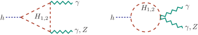
Figure 1: Feynman diagrams for the contributions of the new charged scalars $H_{1,2}^{\pm}$ to the Higgs boson decays $h\to\gamma\gamma$, and $h\to\gamma Z$. The triangle diagram with the gauge boson legs interchanged is not shown.

We can already test the new contributions to $h\rightarrow\gamma\gamma$, which has been observed at the LHC, unlike the $\gamma Z$ channel. For the $\gamma\gamma$ signal strengths, the ATLAS and CMS Collaborations measured $\sigma/\sigma_{\mathrm{SM}}=1.17\pm 0.27$ Aad:2014eha and $1.13\pm 0.24$ CMS:2014ega , respectively. These numbers need to be respected by the ratio of $\Gamma(h\rightarrow\gamma\gamma)$ to its SM value,

$$\mathcal{R}_{\gamma\gamma}=\frac{\Gamma(h\rightarrow\gamma\gamma)}{\Gamma(h\rightarrow\gamma\gamma)_{\mathrm{SM}}}\;.$$ (27)

Its $\gamma Z$ counterpart,

$$\mathcal{R}_{\gamma Z}=\frac{\Gamma(h\rightarrow\gamma Z)}{\Gamma(h\rightarrow\gamma Z)_{\mathrm{SM}}}\;,$$ (28)

will be probed by future experiments.

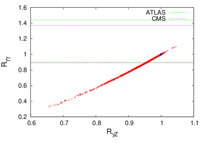
Figure 2: The effects of the new charged scalars $H_{1,2}^{\pm}$ on the ratios of the rates of Higgs decay channels $h\rightarrow\gamma\gamma$ and $h\rightarrow\gamma Z$ to their respective SM values for 5000 benchmark points as described in the text. The blue point marks the SM value. The region between the green (magenta) horizontal lines represents the one-sigma range of the ATLAS (CMS) data Aad:2014eha ; CMS:2014ega .

To illustrate the effects of the inert scalars on $\mathcal{R}_{\gamma\gamma}$ and $\mathcal{R}_{\gamma Z}$, and possible (anti)correlation between them, we display in figure 2 the distribution of 5000 benchmark points on the $(\mathcal{R}_{\gamma Z},\mathcal{R}_{\gamma\gamma})$ plane which satisfy the vacuum stability requirements in eq. (16), the constraints from $W$ and $Z$ decays in eq. (19), and the parameter limitations in eq. (20). We notice that many of the $\mathcal{R}_{\gamma\gamma}$ values are close to 1 and within the allowed ranges from ATLAS and CMS. The plot also reveals that for the $\mathcal{R}_{\gamma\gamma}$ points compatible with the LHC data the values of $\Gamma(h\rightarrow\gamma Z)$ do not differ from its SM value by more than 10% or so. Furthermore, there is a positive correlation between $\mathcal{R}_{\gamma\gamma}$ and $\mathcal{R}_{\gamma Z}$, which is much like the situations in a different recent model with two inert doublets Fortes:2014dia and in the case of only one inert doublet Ho:2013hia ; Swiezewska:2012eh ; Banik:2014cfa . This can be checked experimentally when the $\gamma Z$ mode is observed in the future.

IV Electroweak Precision Tests

The interactions of the new doublets with the SM gauge bosons described by eq. (III) bring about modifications, $\Delta S$ and $\Delta T$, to the so-called oblique electroweak parameters $S$ and $T$ which encode the effects of new physics not directly coupled to SM fermions Peskin:1991sw . At the one-loop level Peskin:1991sw ; pdg

$$\frac{\alpha\Delta S}{4c_{\mathrm{w}}^{2}s_{\mathrm{w}}^{2}} =\frac{A_{ZZ}\left(m_{Z}^{2}\right)-A_{ZZ}(0)}{m_{Z}^{2}}-A_{\gamma\gamma}^{\prime}(0)-\frac{c_{\mathrm{w}}^{2}-s_{\mathrm{w}}^{2}}{c_{\mathrm{w}}s_{\mathrm{w}}}A_{\gamma Z}^{\prime}(0),$$

$$\alpha\Delta T =\frac{A_{WW}(0)}{m_{W}^{2}}-\frac{A_{ZZ}(0)}{m_{Z}^{2}},$$ (29)

where the functions $A_{XY}\left(q^{2}\right)$ can be extracted from the vacuum polarization tensors $\Pi_{XY}^{\mu\nu}\left(q^{2}\right)=A_{XY}\left(q^{2}\right)g^{\mu\nu}+[q^{\mu}q^{\nu}\mathrm{\;terms}]$  of the SM gauge bosons due to the new scalars’ loop contributions, and $A_{XY}^{\prime}(0)=[dA_{XY}\left(q^{2}\right)/dq^{2}]_{q^{2}=0}$. In our numerical analysis below, we will impose

$$\Delta S=0.05\pm 0.11,~{}~{}~{}~{}~{}\Delta T=0.09\pm 0.13,$$ (30)

which are based on the results of a recent fit Baak:2014ora to electroweak precision data for a Higgs mass $m_{h}=125$ GeV.

The contributions of the inert scalars to $\Delta S$ and $\Delta T$ arise from the diagrams depicted in figure 3. After evaluating them, we arrive at

$$\Delta S =\frac{1}{6\pi}\left[\ln\frac{m_{\chi_{1}}m_{\chi_{2}}}{m_{H_{1}^{\pm}}m_{H_{2}^{\pm}}}+s_{2\theta}^{2}\frac{22m_{\chi_{1}}^{2}m_{\chi_{2}}^{2}-5m_{\chi_{1}}^{4}-5m_{\chi_{2}}^{4}}{6\left(m_{\chi_{1}}^{2}-m_{\chi_{2}}^{2}\right)^{2}}\right.$$

$$\hskip 34.44434pt\left.+\;s_{2\theta}^{2}\frac{\left(m_{\chi_{1}}^{2}+m_{\chi_{2}}^{2}\right)\left(m_{\chi_{1}}^{4}-4m_{\chi_{1}}^{2}m_{\chi_{2}}^{2}+m_{\chi_{2}}^{4}\right)}{\left(m_{\chi_{1}}^{2}-m_{\chi_{2}}^{2}\right)^{3}}\ln\frac{m_{\chi_{1}}}{m_{\chi_{2}}}\right],$$ (31)

$$\Delta T =\frac{1}{8\alpha_{\;}\!\pi^{2}v^{2}}\left[c_{\theta}^{2}\mathcal{F}\left(m_{H_{1}^{\pm}},m_{\chi_{1}}\right)+c_{\theta}^{2}\mathcal{F}\left(m_{H_{2}^{\pm}},m_{\chi_{2}}\right)+s_{\theta}^{2}\mathcal{F}\left(m_{H_{1}^{\pm}},m_{\chi_{2}}\right)\right.$$

$$\hskip 51.6665pt\left.+s_{\theta}^{2}\mathcal{F}\left(m_{H_{2}^{\pm}},m_{\chi_{1}}\right)-4c_{\theta}^{2}s_{\theta}^{2}\mathcal{F}\left(m_{\chi_{1}},m_{\chi_{2}}\right)\right],$$ (32)

where

$$\mathcal{F}(m,n)=\frac{m^{2}+n^{2}}{2}-\frac{m^{2}n^{2}}{m^{2}-n^{2}}\ln\frac{m^{2}}{n^{2}}.$$ (33)

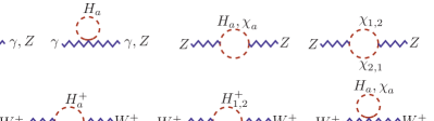
Figure 3: Feynman diagrams for the contributions of the inert scalar doublets to the oblique electroweak parameters $\Delta S$ and $\Delta T$.

In figure 4, we present the distribution on the $(\Delta S,\Delta T)$ plane of the inert scalars’ contributions for the 5000 benchmarks employed previously for figure 2. Evidently, it is possible for the masses of the charged scalars to be as small as 100 GeV and still be compatible with the electroweak precision measurements. However, we find that the lighter one of the inert neutral scalars, $\chi_{1}$, must be heavier than about 90 GeV, which is a stronger condition than that inferred from the LEP constraint on the invisible width of the $Z$ boson. This also makes the bound from the data on the Higgs invisible/nonstandard decay irrelevant.

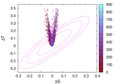
Figure 4: The contributions of the inert scalar doublets to the oblique electroweak parameters $\Delta S$ and $\Delta T$ for the 5000 benchmarks used previously. On the left panel, the palette belongs to the lighter neutral inert scalar’s mass, $m_{\chi_{1}}$, in GeV. On the right panel, the palette belongs to the lighter charged scalar mass, $m_{H_{1}}$, in GeV. The different contours represent 68%, 95%, and 99% confidence level, respectively. The blue point at (0,0) marks the SM value.

V Higgs Trilinear Coupling

Since the new scalars couple directly to the Higgs boson, their presence can cause its trilinear self-coupling, $\lambda_{hhh}$, to shift from its SM prediction. Such a modification could translate into detectable collider signatures, especially at a future $e^{+}e^{-}$ machine such as the International Linear Collider ILCnew where the coupling can be measured with 20% precision or better at a center-of-mass energy $\sqrt{s}=500$ GeV if the integrated luminosity is $500\;\mathrm{fb}^{-1}$.

To derive the formula for the mass-dimension Higgs trilinear self-coupling in the presence of extra heavy particles, we follow the steps taken in ref. AAN . It is just the third derivative of the Higgs effective potential, namely

$$\lambda_{hhh}=\left.\frac{\partial^{3}}{\partial\varphi^{3}}V_{\mathrm{\mathrm{eff}}}^{T=0}(\varphi)\right|_{\varphi=v},$$ (34)

where $\varphi$ is the classical Higgs field and $V_{\mathrm{\mathrm{eff}}}^{T=0}(\varphi)$ is the potential evaluated at temperature $T=0$. We estimate the potential at the one-loop level in the so-called $\overline{\mathrm{DR}}{}^{\prime}$ scheme NaLa ; Martin:2001vx where it has the form

$$V_{\mathrm{eff}}^{T=0}(\varphi)=\frac{\mu_{1}^{2}}{2}\varphi^{2}+\frac{\lambda_{1}}{8}\varphi^{4}+\sum_{i}n_{i}\frac{\left(m_{i}^{2}(\varphi)\right)^{2}}{64\pi^{2}}\left(\ln\frac{m_{i}^{2}(\varphi)}{\Lambda^{2}}-\frac{3}{2}\right).$$ (35)

In the sum above, the index $i$ runs over all the contributing particles, $n_{i}$ stands for the number of internal degrees of freedom of the $i$th particle, with a minus sign added if it is a fermion, $m_{i}^{2}(\varphi)$ is its field-dependent squared mass, and $\Lambda$ is the renormalization scale which we choose to be the Higgs mass, $\Lambda=125.1$ GeV. More explicitly, $n_{h}=1$, $n_{\mathcal{G}}=n_{Z}=n_{\gamma}=3$, $n_{W}=6$, $n_{t}=-12$, and $n_{\chi_{a}}=n_{H_{a}^{\pm}}=2$, where $\mathcal{G}$ refers to the Goldstone bosons. We have collected the formulas for the various relevant $m_{i}^{2}(\varphi)$ in appendix C.

At tree level we have $\mu_{1}^{2}=-\lambda_{1}v^{2}/2\equiv\hat{\mu}_{1}^{2}$, but it receives the one-loop correction

$$\delta\mu_{1}^{2}=-\frac{1}{32\pi^{2}v}\sum_{i}\left.n_{i}m_{i}^{2}\dot{m}_{i}^{2}\left(\ln\frac{m_{i}^{2}}{\Lambda^{2}}-1\right)\right|_{\varphi=v},$$ (36)

which follows from $\partial V_{\mathrm{eff}}^{T=0}(\varphi)/\partial\varphi=0$ set at $\varphi=v\simeq 246~{}\mathrm{GeV}$, where $m_{i}^{2}\equiv m_{i}^{2}(\varphi)$ and $\dot{m}_{i}^{2}\equiv\partial m_{i}^{2}/\partial\varphi$. Then the Higgs mass at the one-loop level, which is nothing but the second derivative of $V_{\mathrm{\mathrm{eff}}}^{T=0}(\varphi)$, is given by

$$m_{h}^{2}=\lambda_{1}v^{2}+\left.\sum_{i}\frac{n_{i}}{32\pi^{2}}\Bigg{[}\Bigg{(}\ddot{m}_{i}^{2}m_{i}^{2}-\frac{\dot{m}_{i}^{2}m_{i}^{2}}{v}+\big{(}\dot{m}_{i}^{2}\big{)}^{2}\Bigg{)}\ln\frac{m_{i}^{2}}{\Lambda^{2}}-\ddot{m}_{i}^{2}m_{i}^{2}+\frac{\dot{m}_{i}^{2}m_{i}^{2}}{v}\Bigg{]}\right|_{\varphi=v},$$ (37)

where the first term is the familiar tree-level contribution, the second term is the radiative one-loop correction, and $\ddot{m}_{i}^{2}\equiv\partial^{2}m_{i}^{2}/\partial\varphi^{2}$. Accordingly, with $m_{h}^{2}$ being fixed to its empirical value, as $\lambda_{1}$ is varied along with the other scalar couplings it can be bigger or smaller than its tree-level value $\hat{\lambda}_{1}=m_{h}^{2}/v^{2}\simeq 0.258$, depending on the size and sign of the loop contribution in eq (37).

Incorporating eq. (37) into eq. (34), one then obtains

$$\lambda_{hhh} =\frac{3m_{h}^{2}}{v}+\frac{1}{32\pi^{2}}\sum_{i=\mathrm{all}}n_{i}\Bigg{\{}\Bigg{[}\dddot{m}_{i}^{2}m_{i}^{2}+3\Bigg{(}\dot{m}_{i}^{2}-\frac{m_{i}^{2}}{v}\Bigg{)}\Bigg{(}\ddot{m}_{i}^{2}-\frac{\dot{m}_{i}^{2}}{v}\Bigg{)}\Bigg{]}\ln\frac{m_{i}^{2}}{\Lambda^{2}}$$

$$~{}~{}~{}~{}+\frac{\left(\dot{m}_{i}^{2}\right)^{3}}{m_{i}^{2}}-\dddot{m}_{i}^{2}m_{i}^{2}+\frac{3m_{i}^{2}}{v}\Bigg{(}\ddot{m}_{i}^{2}-\frac{\dot{m}_{i}^{2}}{v}\Bigg{)}\Bigg{\}}\Bigg{|}_{\varphi=v},$$ (38)

where $\dddot{m}_{i}^{2}\equiv\partial^{3}m_{i}^{2}/\partial\varphi^{3}$. Its SM counterpart, $\lambda_{hhh}^{\mathrm{SM}}$, has the same formula, except that in the sum $i$ runs over SM fields only.

According to eq. (38) and appendix C, the Higgs trilinear self-coupling is a function of the couplings $\lambda_{3a}+\lambda_{4a}$ and $\lambda_{3a}$ of the inert neutral and charged scalars, respectively, to the SM Higgs doublet, i.e. through the field-dependent masses and their derivatives. Since $\lambda_{3a,4a}$ are related to the scalars’ physical masses via eqs. (4) and (13), the Higgs trilinear coupling also depends on them. To illustrate how the inert scalars’ couplings and masses affect $\lambda_{hhh}$, we define the relative change

$$\Delta=\frac{\lambda_{hhh}-\lambda_{hhh}^{\mathrm{SM}}}{\lambda_{hhh}^{\mathrm{SM}}},$$ (39)

with respect to the SM prediction. Then in figure 5 we graph $\Delta$ versus $|\lambda_{32}+\lambda_{42}|$ and $|\lambda_{32}|$, respectively, for the 5000 benchmark points employed earlier. On the same plots we also show the mass distributions of the inert neutral and charged scalars, respectively.

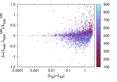
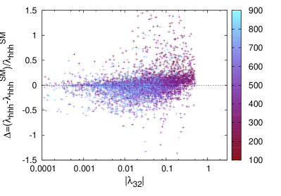
Figure 5: The changes of the Higgs trilinear self-coupling relative to its SM value versus the absolute values of the SM Higgs doublet couplings, $\lambda_{32}+\lambda_{42}$ and $\lambda_{32}$, to the heavy neutral (left) and the heavy charged (right) scalars, respectively. On the palettes, we read the heavy neutral (left) and charged (right) scalar masses in GeV.

It is clear that in the presence of the inert doublets the trilinear Higgs self-coupling can be enhanced or reduced by up to roughly 150% relative to the SM contribution to it. One realizes that, for either large or small (charged and/or neutral) scalar masses and couplings to the SM Higgs doublet, this enhancement or reduction of the trilinear coupling is the effect of the superposition of different contributions which could be constructive or destructive.

The new scalars’ impact can be further seen in figure 6, which illustrates their loop effects. Specifically, it displays the relative changes of the trilinear Higgs coupling, the Higgs mass, and the parameter $\mu_{1}^{2}$ due to radiative corrections versus the Higgs quartic self-coupling $\lambda_{1}$, where

$$\delta\lambda_{hhh}=\lambda_{hhh}-3\lambda_{1}v,~{}~{}~{}~{}~{}\delta m_{h}^{2}=m_{h}^{2}-\lambda_{1}v^{2},$$ (40)

$\delta\mu_{1}^{2}$ is defined in eq. (36), and $\mu_{1}^{2}=\hat{\mu}_{1}^{2}+\delta\mu_{1}^{2}$.

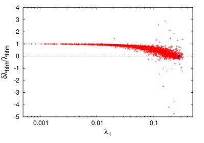
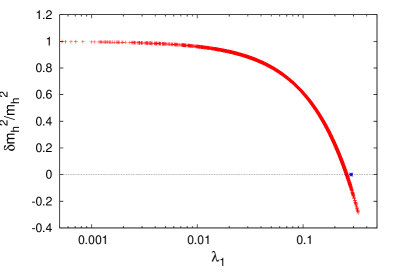
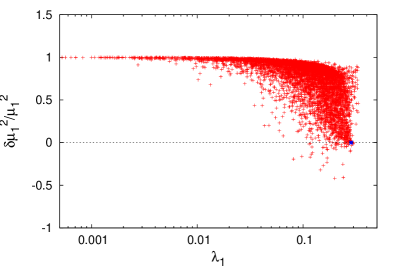
Figure 6: The relative changes of the trilinear Higgs self-coupling (left), the Higgs mass (right) and the $\mu_{1}^{2}$ parameter (bottom) due to loop corrections versus the Higgs quartic self-coupling $\lambda_{1}$. The Higgs mass $m_{h}$ is fixed to 125.1 GeV. The blue points represent the SM values.

We remark that the Higgs quartic self-coupling, which at tree level is defined by the Higgs mass, can have a wide range from about $10^{-4}$ to $0.5$. This is due to the fact that much of the Higgs mass arises radiatively, as the right plot in figure 6 indicates. More precisely, $m_{h}$ can be fully radiative for small $\lambda_{1}$ values or get a negative radiative correction for large $\lambda_{1}$ values, those greater than its tree-level one, $\hat{\lambda}_{1}$. One can see from the top-left and bottom plots in the figure that similar remarks could be made concerning $\lambda_{hhh}$ and $\mu_{1}^{2}$. In particular, each of these parameters may be fully radiative for small $\lambda_{1}$ and also can receive radiative corrections which are negative.

VI Electroweak Phase Transition

It is well-known that one of the reasons why the SM fails to produce successful baryogenesis EWB is the fact that the EWPT is not strong and consequently cannot suppress processes that violate the conservation of baryon plus lepton numbers, $B$+$L$, in the broken phase Trodden:1998ym . The suppression of anomalous $B$+$L$-violating processes in the broken phase happens if the criterion for strongly first-order EWPT SFOPT ; Shaposhnikov:1987pf ,

$$v_{c}/T_{c}>1,$$ (41)

is fulfilled, where $v_{c}$ is the Higgs VEV at the critical temperature $T_{c}$ at which the effective potential exhibits two degenerate minima, one at zero and the other at $v_{c}$. Both $T_{c}$ and $v_{c}$ are determined using the full thermal effective potential Th ; Weinberg:1974hy

$$V_{\mathrm{eff}}(\varphi,T)=V_{\mathrm{eff}}^{T=0}(\varphi)+\frac{T^{4}}{2\pi^{2}}\sum_{i}n_{i}J_{\mathsf{B},\mathsf{F}}\big{(}m_{i}^{2}(\varphi)/T^{2}\big{)}$$ (42)

at a finite temperature $T$, where

$$J_{\mathsf{B},\mathsf{F}}\left(r\right)=\int_{0}^{\infty}dx\;x^{2}\ln\Big{[}1\mp\exp\Big{(}\mbox{$-\sqrt{x^{2}+r}$}\Big{)}\Big{]},$$ (43)

the upper (lower) sign referring to a boson (fermion). To $V_{\mathrm{eff}}(\varphi,T)$ one should add the so-called daisy (or ring) contribution ring

$$V_{\mathrm{ring}}(\varphi,T)=-\frac{T}{12\pi}\sum\limits_{i}n_{i}\bigl{(}\tilde{m}_{i}^{3}(\varphi,T)-m_{i}^{3}(\varphi)\bigr{)}$$ (44)

which represents the leading term of higher-order loop corrections that may play an important role during the EWPT dynamics. In $V_{\mathrm{ring}}(\varphi,T)$ the sum is over the scalar and longitudinal gauge degrees of freedom, $\tilde{m}_{i}^{2}(\varphi,T)=m_{i}^{2}(\varphi)+\Pi_{i}(T)$ are their thermal squared masses, and $\Pi_{i}(T)$ are the thermal parts of the self energies, which are collected in appendix C. To estimate $V_{\mathrm{ring}}(\varphi,T)$, one performs the resummation of an infinite class of infrared-divergent multiloops diagrams, known as ring diagrams, that describes the dominant contribution of long distances and gives a significant contribution when (almost) massless states appear in the system. In our case, we will include this by following another approach. Rather than adding $V_{\mathrm{ring}}(\varphi,T)$ to $V_{\mathrm{eff}}(\varphi,T)$, we will replace in eq. (42) the field-dependent masses of the scalar and longitudinal gauge degrees of freedom with their thermal masses $\tilde{m}_{i}(\varphi,T)$.

In the criterion for a strong first-order phase transition, eq. (41), the critical temperature $T_{c}$ is the value at which the two minima of the effective potential are degenerate,

$$\left.\frac{\partial}{\partial\varphi}V_{\mathrm{eff}}(\varphi,T_{c})\right|_{\varphi=v_{c}}=0,~{}~{}~{}~{}V_{\mathrm{eff}}(\varphi=v_{c},T_{c})=V_{\mathrm{eff}}(\varphi=0,T_{c}).$$ (45)

In the SM, this leads to a Higgs mass below 42 GeV mhbound , since the ratio $v_{c}/T_{c}$ is inversely proportional to the Higgs quartic coupling $\lambda_{1}$. The strength of the EWPT can be improved if new bosonic degrees of freedom are invoked Chowdhury:2011ga ; Ahriche:2010ny ; Borah:2012pu ; Gil:2012ya , which is the case we are investigating. It is clear from eq. (37) that for large values of the couplings and/or masses of the extra scalars, the one-loop corrections to the Higgs mass could be significant, which allows $\lambda_{1}$ to be smaller and, therefore, fulfills the criterion in eq. (41) without conflicting with the recent Higgs mass measurements mhx ; CMS:2014ega . Here, the relevant couplings are those of the Higgs doublet to the charged scalars, $\lambda_{3a}$, and to the neutral ones, $\lambda_{3a}+\lambda_{4a}$, in the limit $|\lambda_{5}|\ll|\lambda_{3a,4a}|$. The situation may be compared to those in similar setups KNT ; hna ; Ahriche:2012ei ; kristian where extra scalars can help bring about a strongly first-order EWPT by (a) relaxing the Higgs quartic coupling $\lambda_{1}$ to as small as $\mathcal{O}(10^{-4})$ and (b) enhancing the value of the effective potential at the wrong vacuum at the critical temperature without suppressing the ratio $v_{c}/T_{c}$, which relaxes the severe bound on the mass of the SM Higgs.

The integral in eq. (43) is often approximated by a high temperature expansion. However, in order to take into account the effect of all the (heavy and light) degrees of freedom, we will evaluate them numerically.

With the same 5000 benchmark points used previously, in figure 7 we present $v_{c}/T_{c}$ as a function of $T_{c}$ and of the Higgs quartic self-coupling. It is obvious that the criterion for a strongly first-order EWPT is easily satisfied for a large number of benchmarks. Moreover, we find that the daisy contribution to the effective potential tends to weaken the EWPT strength in this setup. One also notices that a strong EWPT can be obtained for different values of the Higgs quartic self-coupling $\lambda_{1}$, as shown in the right panel of figure 7, even for values larger than the tree-level one, $\hat{\lambda}_{1}$. This leads us to conclude that the EWPT is always strongly first-order due the reason (b) mentioned above, where the extra heavy scalars’ existence makes the Higgs VEV slowly varying with respect to temperature and the wrong vacuum value, i.e. $V_{\mathrm{eff}}(\varphi=0,T)$, is evolving and increases with temperature.

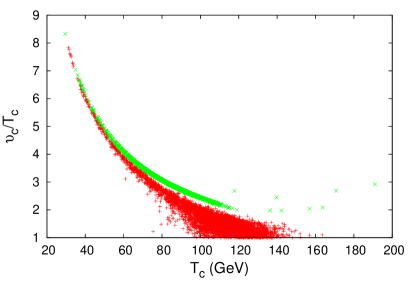
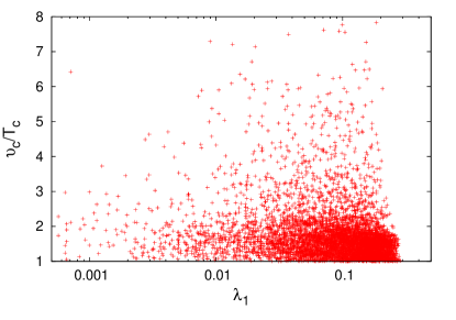
Figure 7: Left panel: $v_{c}/T_{c}$ versus $T_{c}$, estimated with (red) and without (green) the daisy contribution. Right panel: $v_{c}/T_{c}$ versus the Higgs quartic self-coupling $\lambda_{1}$, estimated by considering the daisy contribution.

We remark that due to the absence of a $CP$-violating phase in the potential $\mathcal{V}$ an additional source of $CP$ violation has to be included in the Lagrangian of the more complete theory for it to be realistic for baryogensis. One possibility is to introduce dimension-six operators which couple the inert scalars to the top-quark mass and are suppressed by a new-physics scale that can be well above one TeV, in analogy to a scenario of electroweak baryogenesis from a singlet scalar Cline .

VII Discussion & Conclusion

According to the analysis carried out in previous sections, the extra scalars can have important effects on the Higgs phenomenology and the electroweak phase transition if these particles are relatively light and the couplings to the SM Higgs doublet are large ($\lambda_{3a}$ for charged scalars and $\lambda_{3a}+\lambda_{4a}$ for neutral ones). Therefore, from the 5000 benchmark points used previously, we extract those that simultaneously satisfy (i) the constraint from the measurements on the Higgs decay mode $h\rightarrow\gamma\gamma$, namely $0.9<\mathcal{R}_{\gamma\gamma}<1.37$, (ii) the electroweak precision tests, i.e. all the points inside the three ellipsoids in figure 4, and (iii) the criterion $v_{c}/T_{c}>1$ for strongly first-order EWPT. As mentioned in section IV, the Higgs decay channel into a pair of inert scalars is closed for all the viable benchmarks and hence its experimental bound is not relevant. Here, we divide the points fulfilling the conditions (i,ii,iii) into three sets according to the ellipsoid to which they belong on the $(\Delta S,\Delta T)$ plane. The results are displayed in figure 8.

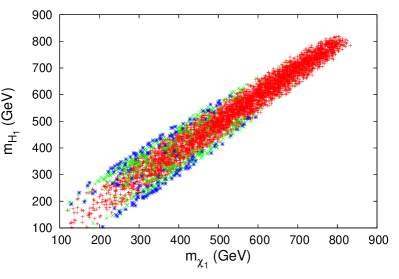
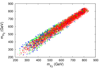
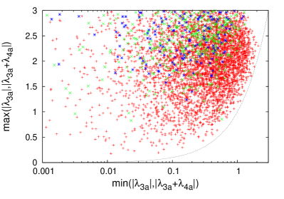
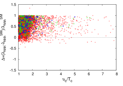
Figure 8: Top panels: the distribution of masses of the extra charged and neutral scalars under the assumptions described in the text. Bottom left panel: the strength distribution of the different quartic self-coupling of the Higgs doublet to the extra charged and neutral scalars; the dashed line represents the case where the couplings are equal in magnitude, i.e., $\mathrm{Min}(|\lambda_{3a}|,|\lambda_{3a}+\lambda_{4a}|)=\mathrm{Max}(|\lambda_{3a}|,|\lambda_{3a}+\lambda_{4a}|)$. Bottom right panel: the EWPT strength versus the relative enhancement of the Higgs trilinear self-coupling. The red, green, and blue points correspond to those inside the 99%, 95%, and 68% CL ellipsoids on the $(\Delta S,\Delta T)$ plane in figure 4.

From the top panels in figure 8, one can see that the extra scalar masses do not exceed 900 GeV according to our parameter choices in eq. (20). The charged scalars could be light up to the LEP II bound (100 GeV), while the neutral scalars, which were supposed to be less constrained before, are now not allowed to be less than 120 GeV due to the electroweak precision tests in this model. From the bottom left panel, it is evident that the couplings of the Higgs doublet to the charged scalars, $\lambda_{3a}$, and to the neutral ones, $\lambda_{3a}+\lambda_{4a}$, could be both larger than 1 or smaller than $0.5$. They could vary also within the whole considered range [0:3], or they could be almost equal in absolute values (i.e. close to the dashed curve). The bottom right plot in this figure reveal that, while strongly first-order EWPT occurs for all of the viable benchmark points, only for some of them there is a positive correlation between the EWPT strength and substantial enhancement of the Higgs trilinear self-coupling relative to the SM prediction as shown in ref. KOS .

In conclusion, we have considered a scenario beyond the SM involving three scalar weak doublets and investigated a number of implications of the case where two of the doublets are inert and charged under a dark Abelian gauge symmetry. We looked at the effects of the new scalars on oblique electroweak parameters, the Higgs decay modes $h\rightarrow\gamma\gamma,\gamma Z$, and its trilinear coupling. We also examined how the inert scalars can induce strongly first-order EWPT. Taking into account various theoretical and experimental constraints, we demonstrated that the viable parameter space can all accommodate strongly first-order EWPT and contains regions in which the Higgs trilinear self-coupling is enhanced/reduced by up to 150% compared to its SM value. Future experiments with sufficient precision can test the new scalars’ effects that we have obtained on the Higgs decays $h\rightarrow\gamma\gamma,\gamma Z$ and trilinear coupling.

Appendix A Vacuum stability conditions

We can rewrite the doublets $\Phi$ and $\eta_{1,2}$ and their products according to

$$\Phi=f\hat{\Phi},~{}~{}~{}~{}~{}\hat{\Phi}^{\dagger}\hat{\Phi}=1,~{}~{}~{}~{}~{}~{}~{}\eta_{a}=e_{a}\hat{\eta}_{a},~{}~{}~{}~{}~{}\hat{\eta}_{a}^{\dagger}\hat{\eta}_{a}=1\;,~{}~{}~{}~{}~{}~{}~{}f,e_{a}>0,$$

$$\hat{\Phi}^{\dagger}\hat{\eta}_{a}\hat{\eta}_{a}^{\dagger}\hat{\Phi}=\rho_{a},~{}~{}~{}~{}~{}~{}~{}\hat{\eta}_{1}^{\dagger}\hat{\eta}_{2}\hat{\eta}_{2}^{\dagger}\hat{\eta}_{1}=\rho^{\prime},~{}~{}~{}~{}~{}~{}~{}0\leq\rho_{a},\rho^{\prime}\leq 1.~{}~{}~{}~{}~{}~{}~{}$$ (46)

Assuming that $\lambda_{5}$ in eq. (II.1) is negligible compared to the other $\lambda$’s, we can then express the part of $\mathcal{V}$ that is quartic in the doublets approximately as

$$\mathcal{V}_{4} =\tfrac{1}{2}\lambda_{1}f^{4}+\tfrac{1}{2}\lambda_{21}e_{1}^{4}+\tfrac{1}{2}\lambda_{22}e_{2}^{4}+\lambda_{31}f^{2}e_{1}^{2}+\lambda_{32}f^{2}e_{2}^{2}$$

$$~{}~{}~{}+\;\lambda_{41}f^{2}e_{1}^{2}\rho_{1}+\lambda_{42}f^{2}e_{2}^{2}\rho_{2}+\lambda_{6}e_{1}^{2}e_{2}^{2}+\lambda_{7}e_{1}^{2}e_{2}^{2}\rho^{\prime}$$

$$=\tfrac{1}{2}\left(\begin{array}[c]{ccc}f^{2}&e_{1}^{2}&e_{2}^{2}\end{array}\right)\tilde{\lambda}\left(\begin{array}[c]{c}f^{2}\vspace{1pt}\\ e_{1}^{2}\vspace{1pt}\\ e_{2}^{2}\end{array}\right),$$ (51)

where

$$\tilde{\lambda}=\left(\begin{array}[c]{ccccc}\lambda_{1}&&\lambda_{31}+\rho_{1}\lambda_{41}&&\lambda_{32}+\rho_{2}^{\;\;}\lambda_{42}\vspace{2pt}\\ \lambda_{31}+\rho_{1}\lambda_{41}&&\lambda_{21}&&\lambda_{6}+\rho^{\prime}\lambda_{7}\vspace{2pt}\\ \lambda_{32}+\rho_{2}^{\;\;}\lambda_{42}&&\lambda_{6}+\rho^{\prime}\lambda_{7}&&\lambda_{22}\end{array}\right).$$ (52)

To ensure the stability of the vacuum, we need to derive relations among the $\lambda$’s in $\mathcal{V}_{4}$, which dominates $\mathcal{V}$ at large fields, such that the minimum of $\mathcal{V}_{4}$ remains positive. This can be achieved using copositivity criteria Kannike:2012pe , which in this case are applied to the minimum of $\tilde{\lambda}$. Since $\lambda_{4a,7}$ can be positive, zero, or negative and $0\leq\rho_{a},\rho^{\prime}\leq 1$, we have

$$\tilde{\lambda}_{\mathrm{min}}=\left(\begin{array}[c]{ccccc}\lambda_{1}&&\lambda_{31}+\mathrm{Min}\left(0,\lambda_{41}\right)&&\lambda_{32}+\mathrm{Min}\left(0,\lambda_{42}\right)\\ \lambda_{31}+\mathrm{Min}\left(0,\lambda_{41}\right)&&\lambda_{21}&&\lambda_{6}+\mathrm{Min}\left(0,\lambda_{7}\right)\\ \lambda_{32}+\mathrm{Min}\left(0,\lambda_{42}\right)&&\lambda_{6}+\mathrm{Min}\left(0,\lambda_{7}\right)&&\lambda_{22}\end{array}\right).$$ (53)

From the criteria for strictly copositive 3$\times$3 matrices copositivity1 ; copositivity2 ; copositivity3 then follow the conditions in eq. (16).

Appendix B Interaction terms for $\mathcal{S}_{a}$ and $\mathcal{P}_{a}$

The interaction terms of $\chi_{1,2}$ in eqs. (III) and (21) can be rewritten in terms of the real and imaginary components defined in eq. (14). Thus

$$\mathcal{L} \supset\frac{g}{2c_{\mathrm{w}}}\Big{[}c_{2\theta}\Big{(}\mathcal{P}_{1}\raisebox{-0.7pt}{\small$\stackrel{{\scriptstyle\scriptscriptstyle\leftrightarrow}}{{\partial}}$}{}^{\mu}\mathcal{S}_{1}-\mathcal{P}_{2}\raisebox{-0.7pt}{\small$\stackrel{{\scriptstyle\scriptscriptstyle\leftrightarrow}}{{\partial}}$}{}^{\mu}\mathcal{S}_{2}\Big{)}+s_{2\theta}\Big{(}\mathcal{P}_{1}\raisebox{-0.7pt}{\small$\stackrel{{\scriptstyle\scriptscriptstyle\leftrightarrow}}{{\partial}}$}{}^{\mu}\mathcal{S}_{2}+\mathcal{P}_{2}\raisebox{-0.7pt}{\small$\stackrel{{\scriptstyle\scriptscriptstyle\leftrightarrow}}{{\partial}}$}{}^{\mu}\mathcal{S}_{1}\Big{)}\Big{]}Z_{\mu}$$

$$~{}~{}~{}~{}+\frac{ig}{2}\Big{\{}\Big{[}c_{\theta}H_{1}^{+}\raisebox{-0.7pt}{\small$\stackrel{{\scriptstyle\scriptscriptstyle\leftrightarrow}}{{\partial}}$}{}^{\mu}(\mathcal{S}_{1}-i\mathcal{P}_{1})+c_{\theta}H_{2}^{+}\raisebox{-0.7pt}{\small$\stackrel{{\scriptstyle\scriptscriptstyle\leftrightarrow}}{{\partial}}$}{}^{\mu}(\mathcal{S}_{2}+i\mathcal{P}_{2})$$

$$\hskip 50.00008pt+s_{\theta}H_{1}^{+}\raisebox{-0.7pt}{\small$\stackrel{{\scriptstyle\scriptscriptstyle\leftrightarrow}}{{\partial}}$}{}^{\mu}(\mathcal{S}_{2}-i\mathcal{P}_{2})-s_{\theta}H_{2}^{+}\raisebox{-0.7pt}{\small$\stackrel{{\scriptstyle\scriptscriptstyle\leftrightarrow}}{{\partial}}$}{}^{\mu}(\mathcal{S}_{1}+i\mathcal{P}_{1})\Big{]}W_{\mu}^{-}-\mathrm{H.c.}\Big{\}}$$

$$~{}~{}~{}~{}+\frac{g^{2}}{4}\big{(}\mathcal{S}_{1}^{2}+\mathcal{P}_{1}^{2}+\mathcal{S}_{2}^{2}+\mathcal{P}_{2}^{2}\big{)}\left(\frac{Z^{2}}{2c_{\mathrm{w}}^{2}}+W^{+\mu}W_{\mu}^{-}\right)$$

$$~{}~{}~{}~{}+\frac{h}{v}\bigl{[}\bigl{(}c_{\theta}^{2}\mu_{21}^{2}+s_{\theta}^{2}\mu_{22}^{2}-m_{\chi_{1}}^{2}\bigr{)}\bigl{(}\mathcal{S}_{1}^{2}+\mathcal{P}_{1}^{2}\bigr{)}+\bigl{(}c_{\theta}^{2}\mu_{22}^{2}+s_{\theta}^{2}\mu_{21}^{2}-m_{\chi_{2}}^{2}\bigr{)}\bigl{(}\mathcal{S}_{2}^{2}+\mathcal{P}_{2}^{2}\bigr{)}$$

$$\hskip 40.00006pt+s_{2\theta}\bigl{(}\mu_{21}^{2}-\mu_{22}^{2}\bigr{)}\bigl{(}\mathcal{S}_{1}\mathcal{S}_{2}+\mathcal{P}_{1}\mathcal{P}_{2}\bigr{)}\bigr{]}\;.$$ (54)

Appendix C Field-Dependent and Thermal Masses

To estimate the Higgs effective potential, one needs the field-dependent squared masses $m_{i}^{2}(\varphi)$ of all the contributing particles. One also requires the first, second, and third derivatives of $m_{i}^{2}(\varphi)$ to determine the counterterm $\delta\mu_{1}^{2}$ in eq. (36), the one-loop correction to the Higgs mass, and the enhancement of the Higgs trilinear self-coupling.

The field-dependent masses of the electroweak gauge bosons and top quark have their SM values. For the other particles, we have the thermal masses $\tilde{m}_{i}\equiv\tilde{m}_{i}(\varphi,T)$ which are given by

$$\tilde{m}_{\mathcal{G}}^{2} =\mu_{1}^{2}+\tfrac{1}{2}\lambda_{1}\varphi^{2}+\Pi_{\Phi},\hskip 47.36096pt\tilde{m}_{h}^{2}=\mu_{1}^{2}+\tfrac{3}{2}\lambda_{1}\varphi^{2}+\Pi_{\Phi},$$

$$\tilde{m}_{H_{a}^{\pm}}^{2} =\mu_{2a}^{2}+\tfrac{1}{2}\lambda_{{3a}}\varphi^{2}+\Pi_{\eta_{a}},\hskip 25.83325pt\tilde{m}_{\chi_{1,2}}^{2}=\tfrac{1}{2}\Big{(}C_{1}+C_{2}\mp\sqrt{R}\Big{)},$$

$$C_{a} =\mu_{2a}^{2}+\tfrac{1}{2}(\lambda_{3a}+\lambda_{4a})\varphi^{2}+\Pi_{\eta_{a}},~{}~{}~{}R=\left(C_{1}-C_{2}\right)^{2}+4c^{2},~{}~{}c=\tfrac{1}{4}\left|\lambda_{5}\right|\varphi^{2},~{}$$ (55)

and related to $m_{i}(\varphi)$ by $\tilde{m}_{i}^{2}(\varphi,T)=m_{i}^{2}(\varphi)+\Pi_{i}$, where $\Pi_{i}\equiv\Pi_{i}(T)$ denote the thermal parts of the self energies and $\Pi_{\Phi,\eta_{a}}$ are listed below. Hence the Goldstone bosons ($\mathcal{G}$) and the Higgs boson also have the same field-dependent masses as their respective counterparts in the SM. We note that the inert $CP$-even and $CP$-odd neutral scalars mix, leading to equal-mass eigenstates, according to eq. (15).

It is simple to get the first, second, and third derivatives of $m_{i}^{2}(\varphi)$ from eq. (C). For completeness, here we supply them explicitly:

$$\dot{m}_{\mathcal{G}}^{2}(\varphi) =\lambda_{1}\varphi,~{}~{}~{}\dot{m}_{h}^{2}(\varphi)=3\lambda_{1}\varphi,~{}~{}~{}\dot{m}_{H_{a}^{\pm}}^{2}(\varphi)=\lambda_{3a}\varphi,$$

$$\dot{m}_{\chi_{1,2}}^{2}(\varphi) =\frac{1}{2}\left(\dot{C}_{1}+\dot{C}_{2}\mp\frac{\dot{R}}{2\sqrt{R}}\right),$$

$$\dot{C}_{a} =\left(\lambda_{{3a}}+\lambda_{{4a}}\right)\varphi,~{}~{}~{}\dot{c}=\tfrac{1}{2}\left|\lambda_{{5}}\right|\varphi,$$

$$\dot{R} =2\left(\dot{C}_{1}-\dot{C}_{2}\right)\left(C_{1}-C_{2}\right)+8\dot{c}c,$$ (56)

$$\ddot{m}_{\mathcal{G}}^{2}(\varphi) =\lambda_{1},~{}~{}~{}\ddot{m}_{h}^{2}(\varphi)=3\lambda_{1},~{}~{}~{}\ddot{m}_{H_{a}^{\pm}}^{2}(\varphi)=\lambda_{{3a}},$$

$$\ddot{m}_{\chi_{1,2}}^{2}(\varphi) =\frac{1}{2}\left(\ddot{C}_{1}+\ddot{C}_{2}\mp\frac{\ddot{R}}{2\sqrt{R}}\pm\frac{\dot{R}^{2}}{4\sqrt{R^{3}}}\right),$$

$$\ddot{C}_{a} =\lambda_{{3a}}+\lambda_{{4a}},~{}~{}~{}\ddot{c}=\tfrac{1}{2}\left|\lambda_{{5}}\right|,$$

$$\ddot{R} =2\left(\dot{C}_{1}-\dot{C}_{2}\right)^{2}+2\left(\ddot{C}_{1}-\ddot{C}_{2}\right)\left(C_{1}-C_{2}\right)+8\dot{c}^{2}+8\ddot{c}c,$$ (57)

$$\dddot{m}_{\mathcal{G}}^{2}(\varphi) =\dddot{m}_{h}^{2}(\varphi)=\dddot{m}_{H_{a}^{\pm}}^{2}(\varphi)=\dddot{C}_{a}=\dddot{c}=0,$$

$$\dddot{m}_{\chi_{1,2}}^{2}(\varphi) =\mp\frac{1}{4\sqrt{R}}\left(\dddot{R}-\frac{3\dot{R}\ddot{R}}{2R}+\frac{3\dot{R}^{3}}{4R^{2}}\right),$$

$$\dddot{R} =6\left(\ddot{C}_{1}-\ddot{C}_{2}\right)\left(\dot{C}_{1}-\dot{C}_{2}\right)+24\ddot{c}\dot{c}.$$ (58)

Finally, we write down the thermal parts $\Pi_{i}$ of the pertinent self-energies. For the scalar and electroweak bosons kapusta

$$\Pi_{\Phi} =\left(6\lambda_{{1}}+\frac{9}{4}{g}^{2}+\frac{3}{4}g_{Y}^{2}+3y_{t}^{2}+4\lambda_{{31}}+2\lambda_{{41}}+4\lambda_{{32}}+2\lambda_{{42}}\right)\frac{T^{2}}{12},$$

$$\Pi_{\eta_{a}} =\left(\frac{9}{4}{g}^{2}+\frac{3}{4}g_{Y}^{2}+4\lambda_{{3a}}+2\lambda_{{4a}}+6\lambda_{{2a}}+4\lambda_{{6}}+2\lambda_{{7}}+\frac{3}{4}\mathcal{Q}_{\eta_{a}}^{2}g_{D}^{2}\right)\frac{T^{2}}{12},$$

$$\Pi_{W} =\frac{17}{6}g^{2}T^{2},~{}~{}~{}\Pi_{B}=\frac{11}{16}g_{Y}^{2}T^{2},$$ (59)

where $y_{t}$ denotes the top-quark Yukawa coupling and $\mathcal{Q}_{\eta_{a}}=\mathcal{Q}_{C}\eta_{a}$ is the charge of the inert doublet $\eta_{a}$ under U(1)_D. Numerically, since $g_{D}$ is unknown, for definiteness we set $g_{D}=g_{Y}$.

References

• (1) G. Aad et al. [ATLAS Collaboration], Phys. Lett. B 716, 1 (2012) [arXiv:1207.7214 [hep-ex]].
• (2) S. Chatrchyan et al. [CMS Collaboration], Phys. Lett. B 716, 30 (2012) [arXiv:1207.7235 [hep-ex]].
• (3) K.A. Olive et al. [Particle Data Group Collaboration], Chin. Phys. C 38, 090001 (2014).
• (4) J.F. Gunion, H.E. Haber, G.L. Kane, and S. Dawson, The Higgs Hunter’s Guide (Westview Press, Colorado, 2000).
• (5) G.C. Branco, P.M. Ferreira, L. Lavoura, M.N. Rebelo, M. Sher, and J.P. Silva, Phys. Rept. 516, 1 (2012) [arXiv:1106.0034 [hep-ph]].
• (6) I.P. Ivanov, V. Keus, and E. Vdovin, J. Phys. A 45, 215201 (2012) [arXiv:1112.1660 [math-ph]].
• (7) A.C.B. Machado and V. Pleitez, arXiv:1205.0995 [hep-ph].
• (8) V. Keus, S.F. King, and S. Moretti, JHEP 1401, 052 (2014) [arXiv:1310.8253 [hep-ph]].
• (9) E.C.F.S. Fortes, A.C.B. Machado, J. Monta$\tilde{\text{n}}$o, and V. Pleitez, arXiv:1408.0780 [hep-ph].
• (10) M. Maniatis and O. Nachtmann, arXiv:1408.6833 [hep-ph].
• (11) I.P. Ivanov and C.C. Nishi, JHEP 1501, 021 (2015) [arXiv:1410.6139 [hep-ph]].
• (12) S. Moretti and K. Yagyu, arXiv:1501.06544 [hep-ph].
• (13) V. Keus, S.F. King, S. Moretti, and D. Sokolowska, JHEP 1411, 016 (2014) [arXiv:1407.7859 [hep-ph]].
• (14) E. Ma, I. Picek, and B. Radovcić, Phys. Lett. B 726, 744 (2013) [arXiv:1308.5313 [hep-ph]].
• (15) S. Kanemura, Y. Okada, and E. Senaha, Phys. Lett. B 606, 361 (2005) [hep-ph/0411354].
• (16) A. Noble and M. Perelstein, Phys. Rev. D 78, 063518 (2008) [arXiv:0711.3018 [hep-ph]].
• (17) C.W. Chiang and T. Yamada, arXiv:1404.5182 [hep-ph].
• (18) K. Fuyuto and E. Senaha, Phys. Rev. D 90, no. 1, 015015 (2014) [arXiv:1406.0433 [hep-ph]].
• (19) D. Curtin, P. Meade, and C.T. Yu, JHEP 1411, 127 (2014) [arXiv:1409.0005 [hep-ph]].
• (20) S. Kanemura, T. Kasai, and Y. Okada, Phys. Lett. B 471, 182 (1999) [hep-ph/9903289].
• (21) S.Y. Ho and J. Tandean, Phys. Rev. D 89, 114025 (2014) [arXiv:1312.0931 [hep-ph]].
• (22) E. Ma, Phys. Rev. D 73, 077301 (2006) [hep-ph/0601225].
• (23) G. Aad et al. [ATLAS Collaboration], Phys. Rev. D 90, 052004 (2014) [arXiv:1406.3827 [hep-ex]].
• (24) CMS Collaboration, Report No. CMS-PAS-HIG-14-009, July 2014.
• (25) D. Curtin, R. Essig, S. Gori, P. Jaiswal, A. Katz, T. Liu, Z. Liu and D. McKeen et al., Phys. Rev. D 90, 075004 (2014) [arXiv:1312.4992 [hep-ph]].
• (26) A. Falkowski, F. Riva, and A. Urbano, JHEP 1311, 111 (2013) [arXiv:1303.1812 [hep-ph]].
• (27) P.P. Giardino, K. Kannike, I. Masina, M. Raidal, and A. Strumia, JHEP 1405, 046 (2014) [arXiv:1303.3570 [hep-ph]].
• (28) J. Ellis and T. You, JHEP 1306, 103 (2013) [arXiv:1303.3879 [hep-ph]].
• (29) G. Belanger, B. Dumont, U. Ellwanger, J.F. Gunion, and S. Kraml, Phys. Rev. D 88, 075008 (2013) [arXiv:1306.2941 [hep-ph]].
• (30) K. Cheung, J. S. Lee and P. Y. Tseng, Phys. Rev. D 90 (2014) 9, 095009 [arXiv:1407.8236 [hep-ph]].
• (31) G. Aad et al. [ATLAS Collaboration], Phys. Rev. D 90 (2014) 11, 112015 [arXiv:1408.7084 [hep-ex]].
• (32) https://twiki.cern.ch/twiki/bin/view/LHCPhysics/CERNYellowReportPageBR3.
• (33) S.Y. Ho and J. Tandean, Phys. Rev. D 87, 095015 (2013) [arXiv:1303.5700 [hep-ph]].
• (34) C.S. Chen, C.Q. Geng, D. Huang, and L.H. Tsai, Phys. Rev. D 87, 075019 (2013) [arXiv:1301.4694 [hep-ph]].
• (35) B. Swiezewska and M. Krawczyk, Phys. Rev. D 88, no. 3, 035019 (2013) [arXiv:1212.4100 [hep-ph]].
• (36) A.D. Banik and D. Majumdar, Eur. Phys. J. C 74, no. 11, 3142 (2014) [arXiv:1404.5840 [hep-ph]].
• (37) M.E. Peskin and T. Takeuchi, Phys. Rev. D 46, 381 (1992).
• (38) M. Baak et al. [Gfitter Group Collaboration], Eur. Phys. J. C 74, no. 9, 3046 (2014) [arXiv:1407.3792 [hep-ph]].
• (39) R. Barbieri, L.J. Hall, and V.S. Rychkov, Phys. Rev. D 74, 015007 (2006) [hep-ph/0603188].
• (40) H. Baer, et al., ’Physics at the International Linear Collider’, available at: http://lcsim.org/papers/DBDPhysics.pdf
• (41) A. Ahriche, A. Arhrib and S. Nasri, JHEP 1402 (2014) 042 [arXiv:1309.5615 [hep-ph]].
• (42) A.B. Lahanas and D.V. Nanopoulos, Phys. Rept. 145, 1 (1987).
• (43) S.P. Martin, Phys. Rev. D 65, 116003 (2002) [hep-ph/0111209].
• (44) V.A. Kuzmin, V.A. Rubakov, and M.E. Shaposhnikov, Phys. Lett. B 155, 36 (1985).
• (45) M. Trodden, Rev. Mod. Phys. 71, 1463 (1999) [hep-ph/9803479].
• (46) M.E. Shaposhnikov, Nucl. Phys. B 287, 757 (1987).
• (47) M. E. Shaposhnikov, Nucl. Phys. B 299, 797 (1988).
• (48) L. Dolan and R. Jackiw, Phys. Rev. D 9, 3320 (1974).
• (49) S. Weinberg, Phys. Rev. D 9, 3357 (1974).
• (50) M.E. Carrington, Phys. Rev. D 45, 2933 (1992).
• (51) A.I. Bochkarev and M.E. Shaposhnikov, Mod. Phys. Lett. A 2, 417 (1987).
• (52) A. Ahriche and S. Nasri, Phys. Rev. D 83, 045032 (2011) [arXiv:1008.3106 [hep-ph]].
• (53) T.A. Chowdhury, M. Nemevsek, G. Senjanovic, and Y. Zhang, JCAP 1202, 029 (2012) [arXiv:1110.5334 [hep-ph]].
• (54) D. Borah and J.M. Cline, Phys. Rev. D 86, 055001 (2012) [arXiv:1204.4722 [hep-ph]].
• (55) G. Gil, P. Chankowski and M. Krawczyk, Phys. Lett. B 717, 396 (2012) [arXiv:1207.0084 [hep-ph]].
• (56) A. Ahriche and S. Nasri, JCAP 1307, 035 (2013) [arXiv:1304.2055].
• (57) A. Ahriche, Phys. Rev. D 75, 083522 (2007) [hep-ph/0701192].
• (58) A. Ahriche and S. Nasri, Phys. Rev. D 85, 093007 (2012) [arXiv:1201.4614 [hep-ph]].
• (59) A. Ahriche, K.L. McDonald and S. Nasri, in preparation.
• (60) J.M. Cline and K. Kainulainen, JCAP 1301, 012 (2013) [arXiv:1210.4196 [hep-ph]].
• (61) K. Kannike, Eur. Phys. J. C 72, 2093 (2012) [arXiv:1205.3781 [hep-ph]].
• (62) K. Hadeler, Linear Algebra Appl. 49, 79 (1983).
• (63) G. Chang and T.W. Sederberg, Comput. Aided Geom. Des. 11(1), 113-116 (1994).
• (64) L. Ping and F.Y. Yu, Linear Algebra Appl. 194, 109 (1993).
• (65) J.I. Kapusta and C. Gale, Finite-temperature field theory: Principles and applications (Cambridge University Press, Cambridge, 2006).