Fluctuating Nonlinear Spring Model of Mechanical Deformation of Biological Particles

Abstract

We present a new theory for modeling forced indentation spectral lineshapes of biological particles, which considers non-linear Hertzian deformation due to an indenter-particle physical contact and bending deformations of curved beams modeling the particle structure. The bending of beams beyond the critical point triggers the particle dynamic transition to the collapsed state, an extreme event leading to the catastrophic force drop as observed in the force ($F$)-deformation ($X$) spectra. The theory interprets fine features of the spectra: the slope of the FX curves and the position of force-peak signal, in terms of mechanical characteristics — the Young’s moduli for Hertzian and bending deformations $E_{H}$ and $E_{b}$, and the probability distribution of the maximum strength with the strength of the strongest beam $F_{b}^{*}$ and the beams’ failure rate $m$. The theory is applied to successfully characterize the $FX$ curves for spherical virus particles — CCMV, TrV, and AdV.

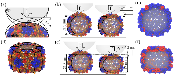
Figure 1: (color) Types of mechanical excitations exemplified using the CCMV shell. (a)-(c) Hertzian deformation $x_{H}$ with normal displacements $u_{tip}$ and $u_{par}$ (scheme on (a)) under the influence of compressive force (vertical arrow). Dashed contour lines show the tip and particle in their undeformed states. Structures in (b) — the native (left) and partially deformed (right) states show the amplitude of $x_{H}$$\approx$$3$ nm. (c) CCMV shell profile showing parts of the structure with high potential energy ($>3$ kcal/mol per residue; red) and low potential energy (blue). (d)-(f) Beam-bending deformation. The side portion of the structure is partitioned into curved vertical beams (top-side view on (d)). Structures in (e) — the partially deformed (left) and pre-collapse (right) states reveal the amplitude of $x_{b}$$\approx$$4.3$ nm. (f) CCMV shell profile under Hertzian and beam-bending deformations showing the potential energy distribution.

Mechanical testing has become the main tool to probe the physico-chemical and materials properties of the protein shells of plant and animal viruses, and bacteriophages RoosNatPhys10 . A variety of viruses have been explored by profiling the indentation force $F$ as a function of particle deformation $X$ ($FX$ curve), including bacteriophages $\Phi 29$ and $HK97$ IvanovskaPNAS04 ; HernandoPerezNano14 ; RoosPNAS12 , the human viruses Noro Virus, Hepatitis B Virus, Human Immuno Deficiency Virus (HIV), Adenovirus (AdV) and Herpes Simplex Virus KolBJ07 ; PerezBernaJBC12 ; RoosPNAS09 ; SnijderJV13 and other eukaryotic cell infecting viruses like Minute Virus of Mice, Triatoma Virus (TrV) and plant viruses Cowpea Chlorotic Mottle Virus (CCMV) and BMV CarrascoPNAS06 ; MichelPNAS06 ; SnijderNC13 ; VaughanJV14 ; NiJMB12 . Although these experiments reveal an amazing diversity of mechanical properties of biological particles, experimental results are difficult to interpret without theoretical modeling. What types of mechanical excitations drive the particle deformation and collapse? What determines the mechanical limit of the particle — the critical forces and critical deformations? Why is the initial portion of the $FX$ spectra weakly non-linear? Why do the $FX$ spectra for the same particle differ from one measurement to another? This points to the stochastic nature of collapse transitions, but what defines the likelihood of structural collapse at a given force load?
A number of theoretical approaches have been designed to describe the dynamics of virus particles, including: finite element analysis GibbonsBJ13 ; KlugPRL12 , normal mode analysis TamaJMB05 , elastic network modeling YangBJ09 , atomistic MD and coarse-grained simulations ZinkBJ10 ; ArkhipovBJ09 ; CieplakJCP10 , and other approaches MayBJ11 . Here we take a step further to develop an analytically tractable model for meaningful interpretation of the force-deformation spectral lineshapes available from single-particle nanomanipulation experiments. The theory links the slope, critical force, and the critical deformation of the $FX$ curve with the physical characteristics of the structure, geometry and overall shape of the particle and indenter. We identify the types of mechanical excitations (degrees of freedom), which contribute to the particle deformation (indentation depth) $X$, by analyzing the structure and potential energy changes in the CCMV particle using our results of nanoindentations in silico. The methodology of nanoindentation in silico is described in Ref.KononovaBJ13 ; see Supplementary Material (SM; Figs. S1-S3). We formulate and apply the Fluctuating Nonlinear Spring (FNS) model to characterize the $FX$ spectra for the CCMV, AdV and TrV particles obtained as described in Refs.SnijderJV13 ; SnijderNC13 ; SnijderMicron12 .
Degrees of freedom — In dynamic force-ramp assays $f(t)$$=$$\kappa\nu_{f}t$, an indenter (cantilever tip) compresses a particle (Fig. 1, S3) creating a physical contact between them. The force loads the particle mechanically over time $t$ with the force-loading rate $\kappa\nu_{f}$ ($\kappa$ and $\nu_{f}$ are the cantilever spring constant and velocity). For small $f$, the mechanical energy is localized to the virion surface under the tip, which results in the tip and particle undergoing normal displacements $u_{tip}$ and $u_{par}$ corresponding to the Hertzian deformation $x_{H}$$=$$u_{tip}$$+$$u_{par}$. Typically, $u_{tip}$$\ll$$u_{par}$, therefore $x_{H}$$=$$u_{par}$. The mechanical energy gradually fills the particle structure stressing the side portions of the structure undergoing bending deformations $x_{b}$ (Fig. 1). The total deformation is the sum of Hertzian and bending deformations, i.e. $X$$=$$x_{H}$$+$$x_{b}$, and the deformation force $F$ of the particle (restoring force exerted on the tip by the particle) is a bivariate function, $F(X$$=$$x_{H}$$+$$x_{b})$$=$$F_{H}(x_{H})$$+$$F_{b}(x_{b})$. We quantified the amplitude of Hertzian deformation $x_{H}$$\approx$$3$ nm and bending deformations $x_{b}$$\approx$$4.3$ nm using the simulation output for the CCMV (Fig. 1).
The Hertz model Landau ; Johnson accounts for the force due to local curvature change $F_{H}(x_{H})$ (Fig. 1(a)),

$$F_{H}(x_{H})=1/D_{H}(R_{par}R_{tip}/(R_{par}+R_{tip}))^{1/2}\cdot x_{H}^{3/2}$$ (1)

where $R_{par}$ and $R_{tip}$ are the radii of the particle and the tip and $D_{H}$$=$$0.75((1-\sigma_{H}^{2})/E_{H}+(1-\sigma_{tip}^{2})/E_{tip})$. $E_{H}$ and $E_{tip}$ are the Young’s moduli and $\sigma_{H}$ and $\sigma_{tip}$ are the Poisson’s ratios for the particle and the tip deformations, respectively. Since $E_{tip}$$\gg$$E_{H}$, $D_{H}$$=$$0.75(1-\sigma_{H}^{2})/E_{H}$. To describe the bending deformations $F_{b}(x_{b})$, we divide the side portion of the particle structure into vertical curved beams of length $L$ (Fig. 1(d)). For a spherical particle with thickness $r$, the total number of beams is $N$$=$$2\pi R_{par}/r$. For small $x_{b}$ (Fig. 1), the potential energy change is $E_{b}I/2\int_{L}(\kappa(x_{b},l)$$-$$\kappa_{0})^{2}dl$ Landau ; Timoshenko , where $\kappa_{0}$ and $\kappa(x_{b},l)$ are the initial and current curvature of the beam element $dl$ ($0$$\leq$$l$$\leq$$R_{par}$$-$$x_{b}/2$) and $E_{b}I$ is the flexural rigidity. With the beam shape function $q(x_{b},l)$$=$$(R_{par}$$+$$x_{b}/2)(1-l^{2}/(R_{par}-x_{b}/2)^{2})^{1/2}$ the curvature of the beam is given by $\kappa(x_{b},l)$$=$$q^{\prime\prime}(x_{b},l)/(1$$+$$(q^{\prime}(x_{b},l))^{2})^{3/2}$ ($q^{\prime}$ and $q^{\prime\prime}$ are the first and second derivatives of $q$ with respect to $l$). By performing the integration we obtain the expression for the beam bending energy, which upon differentiation with respect to $x_{b}$, gives the beam-bending force. Expanding the resulting expression in Taylor series in powers of $x_{b}$ and retaining the linear term we obtain:

$$f_{b}(x_{b})\cong 9E_{b}I\pi/8R_{par}^{3}\cdot x_{b}$$ (2)

Combining the contributions from all $N$ beams and adding together Eqs.(1) and (2), we obtain the deformation force $\tilde{F}(x_{H},x_{b})$$=$$F_{H}(x_{H})$$+$$F_{b}(x_{b})$$=$$k_{H}x_{H}^{3/2}$$+$$Nk_{b}x_{b}$, where $k_{H}$ $=$ $(R_{par}R_{tip}/(R_{par}+R_{tip})^{1/2})/D_{H}$ (Eq.(1)) and $k_{b}$$=$$9E_{b}I\pi/(8R_{par}^{3})$ is the beam spring constant. In agreement with the results of in silico indentation of CCMV (Fig. 2), $F(x_{H},x_{b})$ predicts that the initial portion of $FX$ curves, where Hertzian deformation dominates ($X$$\approx$$x_{H}$), is weakly nonlinear. The Hertzian nonlinearity expressed in $\tilde{F}(x_{H},x_{b})$ was indeed observed in recent experiments on thick-shelled particles MichelPNAS06 . However, $\tilde{F}(x_{H},x_{b})$ does not capture the catastrophic force drop (Fig. 2) because the theory lacks a description of structural damage.
Fluctuating Nonlinear Spring (FNS) model — We represent a particle by a collection of $N$ identical beams interacting with an indenter through a Hertzian cushion. Each $i$-th beam undergoes the equal elastic deformation $x_{bi}$$=$$x_{b}$ with the spring constant ($i$$=$$1,2,\dots,N$) until it fails mechanically when the load on the beam reaches some critical value $f_{bi}^{*}$. The spherical geometry of a virus particle dictates the parallel arrangement of beams with the spring $K_{b}$$=$$\sum_{i=1}^{N}k_{bi}$$=$$Nk_{b}$. There are $n$ (or $N$$-$$n$) beams that have failed (or survived), and the actual bending force is $F_{b}(x_{b})$$=$$k_{b}(N-n)x_{b}$$=$$K_{b}x_{b}(1-n/N)$. We define the random variables associated with the probability of damage $d$$=$$n/N$ and survival $s$$=$$(N-n)/N$$=$$1-d$ of the collection of beams ($0$$\leq$$d$, $s$$\leq$$1$). In the continuous limit, $d$ and $s$ are described by the pdfs $p(F_{b})$, $d(F_{b})$$=$$Prob(F_{b}$$=$$K_{b}x_{b})$$=$$\int_{0}^{F_{b}}p(F_{b}^{\prime})dF_{b}^{\prime}$ and $s(F_{b})$$=$$1-d(F_{b})$$=$$\int_{F_{b}}^{\infty}p(F_{b}^{\prime})dF_{b}^{\prime}$. With the particle damage accounted for, the deformation force becomes:

$$F(x_{H},x_{b})=k_{H}x_{H}^{3/2}+K_{b}x_{b}s(x_{b})$$ (3)

Here, $s$ can be estimated from computer simulations using the structural similarity between a given structure and the initial state $\chi(x_{b})$$=$$(2N(N-1))^{-1}\sum{\Theta(|r_{ij}(x_{b})-r_{ij}(0)|-\beta r_{ij}(0))}$. In the Heaviside step function, $r_{ij}(x_{b})$ and $r_{ij}(0)$ are the distances between the $i$-th and $j$-th amino acids in the given and initial structure, respectively, and $\beta$$=$$0.2$ is the tolerance for the distance change. Because $\chi(x_{b})$ ranges from $\chi$$=$$1$ (fully similar structures) to $\chi$$=$$0$ (completely dissimilar structures) and changes in $s(x_{b})$ are commensurate with structure changes, we have $s(x_{b})$$\approx$$\chi(x_{b})$. The $\chi$-based estimate of $s(x_{b})$ from force-deformation in silico of CCMV shows that this metric can be used to inform the modeling of $p(F_{b})$ (Fig. 2).
The transition to the collapsed state occurs when all beams have failed and so, the longest lasting beam determines the collapse onset at the critical force $F^{col}$ (critical deformation $X^{col}$). Hence, the statistics of the extreme (maximum) force determines the beams’ failure. We used the Weibull distribution Gumbel

$$d(x_{b})=1-e^{-(K_{b}x_{b}/F_{b}^{*})^{m}}\text{, }s(x_{b})=e^{-(K_{b}x_{b}/F_{b}^{*})^{m}}$$ (4)

with the shape parameter $m$ (failure rate), and scale parameter $F_{b}^{*}$ which can be understood by using the condition of maximum force. By substituting $s(x_{b})$ into $F_{b}(x_{b})$ in Eq.(3), by differentiating this expression with respect to $x_{b}$, and by setting $dF_{b}/dx_{b}$$=$$0$, we obtain $F_{b}^{*}$$=$$K_{b}x_{b}^{*}\sqrt[m]{m}$ ($x_{b}^{*}$ is the critical beam deformation). By substituting $F_{b}^{*}$ into the expression for $F_{b}(x_{b})$ and into Eq.(4), we obtain the beam-bending force threshold $F_{b}^{col}$$=$$F_{b}^{*}/\sqrt[m]{em}$$=$$K_{b}x_{b}^{*}/\sqrt[m]{e}$ and the critical value of collapse probability $d^{col}$$=$$1-s^{col}$$=$$1-1/\sqrt[m]{e}$.
By substituting Eq.(4) for $s(x_{b})$ in Eq.(3), we obtain the main result of this Letter:

$$F(x_{H},x_{b})=k_{H}x_{H}^{3/2}+K_{b}x_{b}e^{-(K_{b}x_{b}/F_{b}^{*})^{m}}$$ (5)

Eq.(5) shows that a biological particle behaves as a nonlinear spring. The beams’ bending starts as elastic $(Nk_{b}$), but becomes stochastic near the collapse transition, where the particle mechanical resistance fluctuates, thus explaining the variability of $F^{col}$ and $X^{col}$ in the $FX$ spectra (Figs. 2, 3). Hence, the uniaxial forced deformation of a biological particle can be represented by the mechanical evolution of a fluctuating nonlinear spring (FNS).
Application of FNS model — In the experiment, $F$ is measured as a function of the sum $X$$=$$x_{H}+x_{b}$. A particular realization of the forced deformation process ($FX$ trajectory) is a stochastic path on the 2D surface $F(x_{H},x_{b})$ (Fig. 3). For slow loading, when the particle structure equilibrates on a timescale faster than the rate of force change, the most dominant path is the equilibrium path $F_{eq}(X_{eq})$. Using slow cantilever velocities ($\nu_{f}$$=$$0.06$$-$$1.0$ $\mu$m/s) allows us to use this quasi-equilibrium argument. The equilibrium force $F_{eq}$ can then be determined from the requirement that the deformation force (deformation energy) attains the minimum. Finding $F_{eq}$ is equivalent to finding a pair $x_{H}$ and $x_{b}$ that minimizes $F(x_{H},x_{b})$ subject to the constraint, $X$$=$$x_{H}+x_{b}$ (Fig. 3), which can be solved using Lagrange multipliers (SM).
The average simulated spectra for CCMV are compared with the theoretical curves in Fig. 2 (simulated force-deformation spectra for the CCMV particle are in Fig. S4(a)). To find the best fit, we employed two methods. The exact method is based on Eq.(5) and uses Lagrange multipliers to find $x_{H}$ and $x_{b}$. This requires solving for $x_{b}$ the non-linear equation $a_{1}x_{b}^{4m}+a_{2}x_{b}^{3m}+a_{3}x_{b}^{2m}+a_{4}x_{b}^{m}+a_{5}x_{b}+a_{6}=0$, where $a_{1}$$=$$mK_{b}^{2}(K_{b}/F_{b}^{*})^{4m}$, $a_{2}$$=$$-2m(1+m)K_{b}^{2}(K_{b}/F_{b}^{*})^{3m}$, $a_{3}$$=$$(1+4m+m^{2})K_{b}^{2}(K_{b}/F_{b}^{*})^{2m}$, $a_{4}$$=$$-2(1+m)K_{b}^{2}(K_{b}/F_{b}^{*})^{m}$, $a_{5}$$=$$9/4k_{H}^{2}$, and $a_{6}$$=$$K_{b}^{2}-9/4k_{H}^{2}X$. Then, $x_{H}$ is obtained as $x_{H}$$=$$X$$-$$x_{b}$. In the piece-wise approximate method (Fig. 2), the spectrum is divided into the Hertzian-deformation-dominated initial regime I: $X$$\approx$$x_{H}$ ($x_{b}$$\approx$$0$) and $F$$\approx$$F_{H}$$=$$k_{H}X^{3/2}$; and the transition regime II (non-monotonic part of $FX$ curve): $X$$\approx$$x_{b}$ and $F$$\approx$$F_{b}$$=$$K_{b}Xs(X)$. We calculate $F_{H}$ in regime I for $X$$\approx$$x_{H}$$<$$x_{H}^{max}$; $x_{H}^{max}$ is obtained using Lagrange multipliers and setting $s(x_{b})$$=$$1$. In regime II, we use $F(x_{H}^{max},x_{b})$$=$$k_{H}(x_{H}^{max})^{3/2}+K_{b}(x_{b}-x_{H}^{max}\exp\left[-(K_{b}(x_{b}-x_{H}^{max})/F_{b}^{*})^{m}\right])$ for $X$$\approx$$x_{b}$$>$$x_{H}^{max}$.
The agreement between the simulated force-deformation spectra and theoretical $FX$ curves for the CCMV particle is almost quantitative (Fig. 2); model parameters obtained using both methods are very close (Table I). For all symmetry types, the Hertzian excitation is softer than the beam-bending ($k_{H}$$<$$K_{b}$) implying smaller Young’s modulus for Hertzian deformation, $E_{H}$$<$$E_{b}$, which is why the Hertzian degree of freedom is excited first (Fig. 1). After the Hertzian force reached the maximum $F_{H}^{max}$$=$$k_{H}(x_{H}^{max})^{3/2}$ at $X$$\approx$$x_{H}$$=$$x_{H}^{max}$, a subsequent force increase excites the beam-bending degrees of freedom and $x_{H}$ ($x_{b}$) decreases (increases). Hence, physical properties of the particle are dynamic as the nature of its mechanical response changes with increasing $X$ from Hertzian to beam-bending deformation, because the actual stiffness of beams is degraded with increasing $x_{b}$ as $K_{b}\exp\left[-(K_{b}x_{b}/F_{b}^{*})^{m}\right]$.
The FNS model accounts for the dependence of mechanical response of biological particles on particle and indenter geometries KononovaBJ13 . Since the information about the particle/indenter size is contained in $k_{H}$, geometric effects are important in the Hertzian deformation regime. When $m$$>$$1$ ($m$$<$$1$), the beam failure events become more frequent (less frequent) with increasing $x_{b}$. For CCMV, $1.8$$<$$m$$<$$2.1$ (Table I), which indicates that the beam-failure rate increases with $X$. When first $n$ beams fail, the compressive force is redistributed among the remaining $N-n$ beams, and each surviving beam experiences an increasingly larger tension with every next beam failure, which accelerates the failure frequency. The beams fail not when $f$$>$$F_{b}^{*}$, but under smaller forces $F_{b}^{col}$$=$$F_{b}^{*}/\sqrt[m]{em}$ (for $m$$\approx$$2$, $F_{b}^{col}$$\approx$$0.43F_{b}^{*}$).
The AFM-based measurements for the empty CCMV shell, empty TrV capsid, full TrV virion and full AdV virion are in Figs. S4, S5. Theoretical fit to the experimental average $FX$ curves for these particles shows that their deformations are well described by the FNS model (Fig. 3). The obtained Young’s moduli for Hertzian deformation are uniformly smaller ( $10$$-$$100$ MPa) than the Young’s moduli for bending deformation (Giga-Pascal range; Table I). This correlates with the $FX$ curves being only weakly nonlinear (Fig. 3). There are small variations in the model parameters for the AdV virion due to force application along different symmetry axes. This correlates with our similar findings for the CCMV shell, and implies that the symmetry of local arrangements of capsomer repeats at the point of indentation influences its mechanics KononovaBJ13 . The failure rates are found to be accelerating with deformation ($m$$>$$1$). This fully reflects the conditions of application of compressive force, which increases linearly in time speeding up beams’ failure events. Parameters for empty and ssRNA-loaded TrV capsids indicate that the difference in particle stiffness is largely due to an increase in the Young’s modulus for Hertzian deformation $E_{H}$$=$$0.03$ GPa (empty TrV) vs $0.14$ GPa (full TrV), which suggests that local indentations are resisted in ssRNA-filled particles. These results fit with the previously observed uniaxial deformation of RNA-filled TrV into an oblate sphere to maximize the volume available to pack the genome SnijderNC13 . Hence, confining the large ssRNA genome inside the small particle volume builds internal pressure resisting local indentation.
Previously, the 3D Young’s modulus of the capsid material was estimated using a thin shell theory RoosNatPhys10 ; MichelPNAS06 ; SnijderNC13 ; Landau . This assumption is valid for some bacteriophage capsids, but in CCMV and TrV the shell thickness is comparable with the virion radius. The FNS model accounts for compression of the protein layer under the tip. In the FNS model, the beam-bending modulus ($E_{b}$) is roughly equivalent to the 3D Young’s modulus in the thin shell theory. It is estimated at $\sim$$0.85$ GPa (experiment) and $\sim$$0.4$$-$$0.5$ GPa (simulations) for the empty CCMV capsid (Table I). These are similar to yet larger than the values of $0.15$$-$$0.30$ GPa obtained with the thin shell theory RoosNatPhys10 ; MichelPNAS06 and $0.28$$-$$0.36$ GPa from finite-element analysis ($\sim$$0.25$ GPa) GibbonsPRE07 , but they disagree with the estimates from several computer modeling studies ($0.08$$-$$0.09$ GPa) CieplakJCP10 ; MayBJ11 . In the study based on spherical harmonics MayBJ11 , multiple deformation modes have also been observed, corresponding to equilibrium deformations of the polar regions (tip/surface contact area in FNS model) and the side wall (beams in FNS model) of the shell. For the empty TrV capsid, we obtain $E_{b}$$\approx$$0.9$ GPa (Table I) whereas the thin shell theory gives a smaller value of $\sim$$0.5$ GPa. The lower values of the 3D Young’s modulus result from attributing the softer Hertzian deformation mode to bending of the capsid shell in the thin shell theory. Indeed, for CCMV and TrV shells, the thin shell theory estimates $0.15$$-$$0.30$ GPa and $0.5$ GPa are between the values of $E_{H}$$=$$0.02$$-$$0.03$ GPa and $E_{b}$$=$$0.85$$-$$0.95$ GPa from FNS modeling (Table I).
We used parameters of the FNS model and positions of the force maximum at $X^{col}$$=$$x_{H}^{*}+x_{b}^{*}$ from the $FX$ spectra (Figs. 2, 3) to predict the critical force for collapse, $F^{col}$$=$$F_{H}(x_{H}^{*})+F_{b}^{col}(x_{b}^{*})$$=$$k_{H}x_{H}^{*3/2}+K_{b}x_{b}^{*}/\sqrt[m]{e}$. The obtained values of $F^{col}$ (Table I) agree with their counterparts extracted from the $FX$ curves (Figs. 2, 3), which validates the model. The analytically tractable FNS model uniquely combines the elements of continuum mechanics and statistics of extremes to accurately describe the mechanical deformation and collapse of biological particles. The model can also be extended to characterize the biological particles with other regular geometries, e.g. microtubule polymers (cylinder) DePabloPRL03 ; KononovaJACS14 .

Table 1: Biomechanical and statistical characteristics determining the deformation and collapse of biological particles — CCMV, TrV, and AdV: the Young’s moduli for Hertzian deformation $E_{H}$ and beam-bending $E_{b}$, the force scale parameter $F_{b}^{*}$ and shape parameter $m$. The first (second) entries correspond to the exact (approximate) methods of parameter estimation. The model predictions for $F^{col}$ are compared with the peak forces (in parenthesis) from the spectra (Figs. 2, 3). For TrV and AdV, the shell thickness was estimated in SM.

System	$E_{H}$, GPa	$E_{b}$, GPa	$F_{b}^{*}$, nN	$m$	$F^{col}$, nN
CCMV (2-fold symmetry; in silico)	0.013/0.012	0.50/0.50	1.70/1.25	1.7/1.5	0.67/0.69 (0.68)
CCMV (quasi-2-fold symmetry; in silico)	0.011/0.011	0.37/0.35	1.50/1.25	1.4/1.6	0.58/0.64 (0.68)
CCMV (quasi-3-fold symmetry; in silico)	0.012/0.012	0.52/0.46	1.75/1.33	1.4/1.6	0.58/0.64 (0.68)
empty CCMV (average; in vitro)	0.019/0.023	0.85/0.81	1.90/1.00	1.2/1.3	0.56/0.78 (0.71)
empty TrV (average; in vitro)	0.030/0.036	0.94/0.81	1.90/1.1	1.1/1.2	0.70/1.02 (0.69)
full TrV (average; in vitro)	0.140/0.140	0.95/0.84	8.10/5.5	1.1/1.0	2.91/3.78 (3.00)
full AdV (2-fold symmetry; in vitro)	0.037/0.040	0.35/0.29	10.0/5.0	1.2/1.4	2.58/4.05 (3.80)
full AdV (3-fold symmetry; in vitro)	0.018/0.019	0.20/0.18	11.0/5.0	1.3/1.7	3.04/4.15 (4.30)
full AdV (5-fold symmetry; in vitro)	0.021/0.023	0.14/0.13	5.10/3.7	1.1/1.0	2.03/2.35 (1.90)

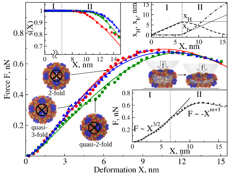
Figure 2: (color) Forced deformation of CCMV shell in silico: the average $FX$ spectra (data points), obtained from the simulations of nanoindentation ($\nu_{f}$$=$$1.0$ $\mu$m/s, $R_{tip}$$=$$20$ nm, and $\kappa$$=$$0.05$ N/m; Fig. S4(a)) along the 2-fold (red), quasi-3-fold (blue), and quasi-2-fold symmetry axes (green), and theoretical $FX$ curves (solid lines). The circled bolded X shows the locations of force application. We used MD simulations accelerated on GPUs ZhmurovProt10 ; ZhmurovJPC11 and nanoindentations in silico of the CCMV capsid KononovaBJ13 (Figs. S1-S3). Structures under the force maxima depict the capsid transitioning from the state before the collapse (left) to the collapsed state (right). The top insets: $\chi$-based estimation of $s(X)$ (left) and dynamics of $x_{H}$ and $x_{b}$ vs. $X$ (right) in the Hertzian regime I and in the transition regime II (dashed and dashed-dotted lines are for the exact method, and solid lines are for the approximate piece-wise method of parameter estimation). The bottom inset: schematic for piece-wise spectrum modeling; regime I — $X$$\approx$$x_{H}$, and $F(X)$$\approx$$F_{H}$; regime II — $X$$=$$x_{H}+x_{b}$ and $F(X)$$=$$F_{H}+F_{b}$.

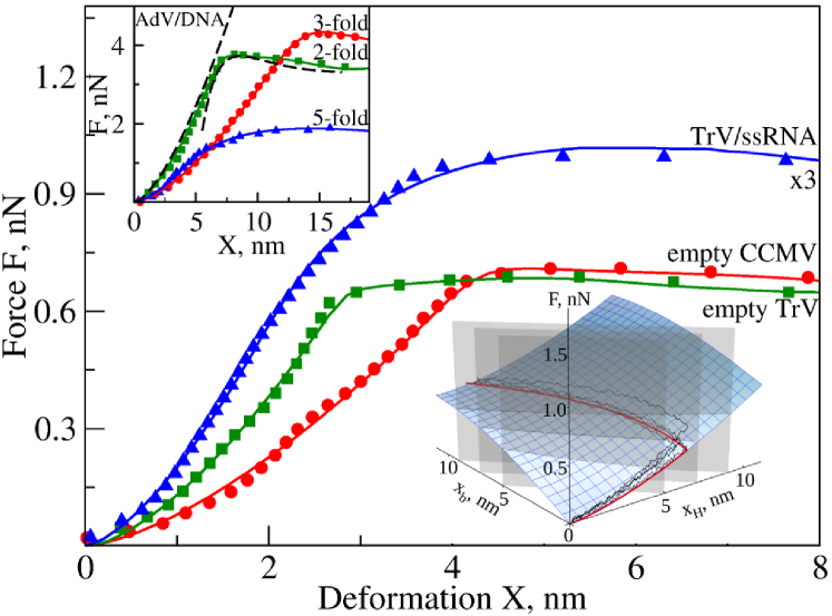
Figure 3: (color) AFM-based forced deformation of empty CCMV and TrV shell, TrV with ssRNA, and AdV with dsDNA (top inset which also shows a schematic for piece-wise modeling); see Figs. S4(b), S5(a) - (c). For empty CCMV, $\nu_{f}$$=$$0.06$ $\mu$m/s, $R_{tip}$$=$$20$ nm, and $\kappa$$=$$0.05$ N/m. For empty TrV, $\nu_{f}$$=$$0.06$ $\mu$m/s, $R_{tip}$$=$$15$ nm, and $\kappa$$=$$0.056$ N/m. For TrV with ssRNA, $\nu_{f}$$=$$0.06$ $\mu$m/s, $R_{tip}$$=$$15$ nm, and $\kappa$$=$$0.1$ N/m. For full AdV with dsDNA, $\nu_{f}$$=$$0.055$ $\mu$m/s, $R_{tip}$$=$$15$ nm, and $\kappa$$=$$0.0524$ N/m. The average experimental spectra (data points) are compared with theoretical $FX$ (solid) curves. The bottom inset shows the 2D surface (Eq.(5)) constructed with the model parameters from CCMV indentation in silico along the 2-fold symmetry axis (Fig. 2; Table I). The red curve is the equilibrium average curve $F_{eq}X_{eq}$ with the points formed by the intersection of $F(x_{H},x_{b})$ with line $x_{b}$$=$$X$$-$$x_{H}$ (shown for $X$$=5,7$, and $9$ nm). The noisy black curves are particular realizations of the stochastic $FX$ path.