Theory of Optical Bloch Oscillations in the Zigzag Waveguide Array

Abstract

The Bloch oscillations in the zigzag array of the optical waveguides are considered. The multiple scattering formalism (MSF) is used for the numerical simulation of the optical beam which propagates within the array. The effect of the second-order coupling which depends on the geometrical parameters of the array is investigated. The results obtained within the MSF are compared with the calculation based on the phenomenological coupling modes model. The calculations are performed for the waveguides fabricated in alkaline earth boro-aluminosilicate glass sample, which are the most promising for the C-band ($\lambda\sim 1530-1565\,\mathrm{nm}$).

I Introduction

The rapid development of technologies for production of optical waveguides provides a possibility of optical simulation of quantum phenomena inherent in the condensed-matter physics Review_Longhi2009 , such as Bloch oscillations Pertsch1998_Theor ; Pertsch1999 ; Morandotti1999 ; Pertsch2002 ; Chiodo2006 ; Gradons_Zheng2010 , Zenner tunneling Trompeter2006 ; Dreisow1_2009 ; Wang1_2010 , Anderson localization AndLoc_Schwartz2008 ; AndLoc_Lahini2008 , dynamic localization DinLoc_Garanovich2007 ; DinLoc_Dreisow2008 . Periodic arrays of optical waveguides are a special case of photonic crystals. Such systems are of interest due to the band structure of their optical spectrum that is similar to the band structure in the electronic spectrum of ordinary crystals Joannopoulos ; Busch . Because of this, the behavior of light in photonic crystals is analogous to the behavior of electron wave function in a periodic potential of ordinary crystals. This fact is of considerable interest for practical applications because it allows to steer the optical signal effectively. Besides, it is interesting from a purely scientific point of view, since the optical counterparts of quantum phenomena can be observed directly.

Usually, the theoretical model of the light propagation in the optical waveguides array takes into account only the next neighbors coupling (NNC). This model is applicable for the particular case of the plane arrays, since the high order coupling is too weak. But sometimes the second-order coupling (SOC) should be taken into account. The most evident example of a system with the significant SOC is the zigzag array (see Fig. 1). For such a system the SOC depends on the angle $\theta$. Varying this angle, we can make the SOC comparable or even greater then the NNC. The SOC can influence the diffraction processes Zigzag_Dreisow2008 and forming of the solitons in the case of the nonlinear optics ZigzagSolitons_Efremidis2002 ; ZigzagSolitons_Szameit2009 .

In this paper we investigate the influence of SOC on the optical Bloch oscillations. The phenomenon of Bloch oscillations (BO) takes place in the array with the monotonic change of the refractive index of the waveguides as one passes from one homogeneous waveguide to another. For the case of the plane array, where only the NNC should be taken into account, the light beam path possesses an oscillatory form. This effect is widely investigated both experimentally and theoretically in Pertsch1998_Theor ; Pertsch1999 ; Morandotti1999 ; Pertsch2002 ; Chiodo2006 . But for the zigzag array, where the SOC is considerable, the path of the optical beam takes more complex form. This phenomenon, known as the anharmonic Bloch oscillation (ABO), was predicted in Wang2010 and experimentally confirmed in Dreisow2011 .

Numerical simulation of various phenomena in systems of interacting optical waveguides, including BO and ABO, is usually based on a coupled modes model. The parameters of this model are typically determined experimentally.

In our works We_OptEng2014 ; We_arXiv13105312 we proposed another method of numerical simulation which requires no additional data except of the geometrical and optical parameters of the array (radii of the waveguides and distances between them, the refractive indices of the waveguides and environment). Our method uses the multiple scattering formalism based on the macroscopic electrodynamics approach. In papers We_OptEng2014 ; We_arXiv13105312 we presented the general algorithm for calculating the path of the optical beam in an array of waveguides.

In the present work we generalize the results obtained in We_OptEng2014 ; We_arXiv13105312 . We apply the multiple scattering formalism to the ABO calculation in the zigzag array. The obtained picture of ABO is compared with the results of calculation with use of the coupling mode model. For this purpose, we derive the analytical formula for the path of the optical beam in the zigzag array, using the coupling mode model with the SOC taken into account. Besides, we use the MSF to obtain the dependence of the coupling constant of the SOC as function of the angle $\theta$ (see Fig. 1).

Recently a new method to fabricate low bend loss femtosecond-laser written waveguides was developed [24, 25]. The waveguides are fabricated in alkaline earth boro-aluminosilicate glass sample, so they are the most effective for the C-band ($\lambda\sim 1530-1565\,\mathrm{nm}$). In this work we consider a sample that can be fabricated by means of this technology.

This paper is organized as follows. In Sec. II we describe the multiple scattering formalism. In subsection II.1 we present the algorithm for calculating the path of the optical beam in an array of waveguides. In subsection II.2 we derive the equation of the coupling modes model from the MSF and present the formulae for the coupling constants. In Sec. III we represent the pictures of ABO obtained by use of MSF for different $\theta$. We compare these results with the paths of the optical beam described by the coupling modes model. Besides, in Sec. III we present the dependence of the SOC coupling constant on the angle $\theta$.

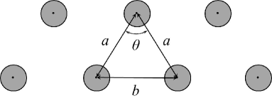
Figure 1: Zigzag optical waveguide array.

II Multiple scattering formalism

Let us consider the array of $N$ parallel infinite cylindrical dielectric waveguides. The axes of the waveguides are parallel to the $z$-axis. The distance between the axes of the adjacent waveguides is denoted by $a$. All the waveguides are assumed to possess the same radius $R$ but different refractive indices $n_{j}$, $j$ being the waveguide number. The refractive index of the environment is $n^{0}$. The permeability of the waveguide material and the environment is unity.

Suppose that a guided mode with a frequency $\omega$ is excited within the array. Then, all the components of the electromagnetic field are proportional to $e^{-i\omega t+i\beta z}$.

Let us consider the field of the guided mode inside of the array. The field of the guided mode is finite in any point into the waveguide. So, the electromagnetic field inside of the $j$-th waveguide may be represented in the form

$$\begin{array}[]{l}\displaystyle\tilde{\mathbf{E}}_{j}(\mathbf{r})=e^{-i\omega t+i\beta z}\,\sum\limits_{m=0,\pm 1...}e^{im\phi_{j}}\,\Bigl{(}c_{jm}\,\tilde{\mathbf{N}}_{\omega_{j}\beta m}(\rho_{j})-d_{jm}\,\tilde{\mathbf{M}}_{\omega_{j}\beta m}(\rho_{j})\Bigr{)},\vskip 6.0pt plus 2.0pt minus 2.0pt\\ \displaystyle\tilde{\mathbf{H}}_{j}(\mathbf{r})=e^{-i\omega t+i\beta z}\,n_{j}\sum\limits_{m=0,\pm 1...}e^{im\phi_{j}}\,\Bigl{(}c_{jm}\,\tilde{\mathbf{M}}_{\omega_{j}\beta m}(\rho_{j})+d_{jm}\,\tilde{\mathbf{N}}_{\omega_{j}\beta m}(\rho_{j})\Bigr{)},\qquad\rho_{j}<R.\end{array}$$ (1)

Here $\omega_{j}=n_{j}\omega$, and $\rho_{j}$, $\phi_{j}$ are the cylindrical coordinates of the vector $\mathbf{r}-\mathbf{r}_{j}$, where $\mathbf{r}_{j}$ is the coordinates of the axis of the $j$-th waveguide. The vector cylinder harmonics $\tilde{\mathbf{M}}_{\omega_{j}\beta m}(\rho_{j})$ and $\tilde{\mathbf{N}}_{\omega_{j}\beta m}(\rho_{j})$ are defined as follows

$$\tilde{\mathbf{N}}_{\omega_{j}\beta m}(\rho_{j})=\mathbf{e}_{r}\,\frac{i\beta}{\varkappa_{j}}\,J^{\prime}_{m}(\varkappa_{j}\rho_{j})-\mathbf{e}_{\phi}\,\frac{m\beta}{\varkappa_{j}^{2}\rho_{j}}\,J_{m}(\varkappa_{j}\rho_{j})+\mathbf{e}_{z}\,J_{m}(\varkappa_{j}\rho_{j}),$$ (2)

$$\tilde{\mathbf{M}}_{\omega_{j}\beta m}(\rho_{j})=\mathbf{e}_{r}\,\frac{m\omega_{j}}{\varkappa_{j}^{2}\rho_{j}}\,J_{m}(\varkappa_{j}\rho_{j})+\mathbf{e}_{\phi}\,\frac{i\omega_{j}}{\varkappa_{j}}\,J^{\prime}_{m}(\varkappa_{j}\rho_{j}),$$ (3)

where $\varkappa_{j}=\sqrt{\omega_{j}^{2}-\beta^{2}}$, $J_{m}(\varkappa_{j}\rho_{j})$ is the Bessel function, and the prime means the derivative with respect to the argument $\varkappa_{j}\rho_{j}$.

Let us turn to the electromagnetic field outside of the array. This field is the sum of the contributions of all the waveguides,

$$\mathbf{E}(\mathbf{r})=\sum\limits_{j=1}^{N}\mathbf{E}_{j}(\mathbf{r}),\qquad\mathbf{H}(\mathbf{r})=\sum\limits_{j=1}^{N}\mathbf{H}_{j}(\mathbf{r}).$$ (4)

The contribution induced by the $j$-th waveguide and vanishing at $\rho_{j}\to\infty$ may be represented in the form

$$\begin{array}[]{l}\displaystyle\mathbf{E}_{j}(\mathbf{r})=e^{-i\omega t+i\beta z}\sum\limits_{m}e^{im\phi_{j}}\,\Bigl{(}a_{jm}\,\mathbf{N}_{\omega^{\prime}\beta m}(\rho_{j})-b_{jm}\,\mathbf{M}_{\omega^{\prime}\beta m}(\rho_{j})\Bigr{)},\vskip 6.0pt plus 2.0pt minus 2.0pt\\ \displaystyle\mathbf{H}_{j}(\mathbf{r})=e^{-i\omega t+i\beta z}n^{0}\sum\limits_{m}e^{im\phi_{j}}\,\Bigl{(}a_{jm}\,\mathbf{M}_{\omega^{\prime}\beta m}(\rho_{j})+b_{jm}\,\mathbf{N}_{\omega^{\prime}\beta m}(\rho_{j})\Bigr{)},\qquad\rho_{j}>R.\end{array}$$ (5)

Here $\omega^{\prime}=n^{0}\omega$. The vector cylinder harmonics $\tilde{\mathbf{M}}_{\omega_{j}\beta m}(\rho_{j})$ and $\tilde{\mathbf{N}}_{\omega_{j}\beta m}(\rho_{j})$ are

$$\mathbf{N}_{\omega^{\prime}\beta m}(\rho_{j})=\mathbf{e}_{r}\,\frac{i\beta}{\varkappa^{\prime}}\,H^{\prime}_{m}(\varkappa^{\prime}\rho_{j})-\mathbf{e}_{\phi}\,\frac{m\beta}{\varkappa^{\prime 2}\rho_{j}}\,H_{m}(\varkappa^{\prime}\rho_{j})+\mathbf{e}_{z}\,H_{m}(\varkappa^{\prime}\rho_{j}),$$ (6)

$$\mathbf{M}_{\omega^{\prime}\beta m}(\rho_{j})=\mathbf{e}_{r}\,\frac{m\omega^{\prime}}{\varkappa^{\prime 2}\rho_{j}}\,H_{m}(\varkappa^{\prime}\rho_{j})+\mathbf{e}_{\phi}\,\frac{i\omega^{\prime}}{\varkappa^{\prime}}\,H^{\prime}_{m}(\varkappa^{\prime}\rho_{j}),$$ (7)

where $\varkappa^{\prime}=\sqrt{\omega^{\prime 2}-\beta^{2}}$, and $H_{m}(\varkappa^{\prime}\rho_{j})$ is the Hankel function of the first kind. Note that, for $\beta=0$, Eqs. (1) and (5) transform into the corresponding expressions in Ref. VanDeHulst , however different notations are used there.

Below we consider the simplest approximation to these equations, namely, the zero-harmonic approximation. This means that in Eqs. (1) and (5) only the terms with $m=0$ are taken into account. In this approximation there are two kinds of the guided modes, namely the transverse magnetic (TM) and transverse electric (TE) modes. For the TM-mode $b_{j0}=d_{j0}=0$, and for the TE-mode $a_{j0}=c_{j0}=0$. As an example, let us consider the TM-modes.

$$\tilde{\mathbf{E}}_{j}(\mathbf{r})=c_{j}\,\tilde{\mathbf{N}}_{\omega_{j}\beta 0}(\rho_{j}),\qquad\tilde{\mathbf{H}}_{j}(\mathbf{r})=c_{j}\,n_{j}\,\tilde{\mathbf{M}}_{\omega_{j}\beta 0}(\rho_{j})\qquad\rho_{j}<R.$$ (8)

$$\mathbf{E}_{j}(\mathbf{r})=a_{j}\,\mathbf{N}_{\omega^{\prime}\beta 0}(\rho_{j}),\qquad\mathbf{H}_{j}(\mathbf{r})=a_{j}\,n^{0}\,\mathbf{M}_{\omega^{\prime}\beta 0}(\rho_{j})\qquad\rho_{j}>R.$$ (9)

Here and below, $a_{j}$ and $c_{j}$ stand for $a_{j0}$ and $c_{j0}$, and the factor $e^{-i\omega t+i\beta z}$ is omitted.

To derive the equations that determine the partial amplitudes $a_{j}$ and $c_{j}$, one should use the boundary conditions on the surface of every waveguide. The boundary conditions on the surface of the $j$-th waveguide connect the field $\tilde{\mathbf{E}}_{j}(\mathbf{r})$, $\tilde{\mathbf{H}}_{j}(\mathbf{r})$ inside the $j$-th waveguide and the field $\mathbf{E}(\mathbf{r})$, $\mathbf{H}(\mathbf{r})$ outside. In general, there are four independent boundary conditions We_arXiv13105312 . However, for $m=0$ TM-modes and only two boundary conditions are required:

$$\left[\mathbf{E}(\mathbf{R}_{j})\right]_{z}=\left[\tilde{\mathbf{E}}_{j}(\mathbf{R}_{j})\right]_{z},\qquad\left[\mathbf{H}(\mathbf{R}_{j})\right]_{\phi}=\left[\tilde{\mathbf{H}}_{j}(\mathbf{R}_{j})\right]_{\phi},$$ (10)

here $\mathbf{R}_{j}$ is the radius-vector of a point on the surface of the $j$-th waveguide.

The boundary conditions on the surface of the $j$-th waveguide can be expressed in the most convenient form if the contributions of all the waveguides to the field outside the array are expressed in terms of the same argument $\rho_{j}$. For this propose we apply the following relations:

$$\begin{array}[]{l}\displaystyle\mathbf{N}_{\omega^{\prime}\beta 0}(\rho_{l})\approx U_{lj}(\omega,\beta)\,\tilde{\mathbf{N}}_{\omega^{\prime}\beta 0}(\rho_{j}),\vskip 6.0pt plus 2.0pt minus 2.0pt\\ \displaystyle\mathbf{M}_{\omega^{\prime}\beta 0}(\rho_{l})\approx U_{lj}(\omega,\beta)\,\tilde{\mathbf{M}}_{\omega^{\prime}\beta 0}(\rho_{j}),\qquad l\neq j,\end{array}$$ (11)

where $U_{lj}(\omega,\beta)=H_{0}(\varkappa^{\prime}r_{lj})$, $H_{0}$ being the Hankel function of the first kind and $r_{lj}$ being the distance between the axes of the $j$-th and the $l$-th waveguides. The relations (11) follow from the Graf theorem (see AbramowitzStegun ) in the zero-harmonic approximation.

Thus, it follows from (9) that

$$\mathbf{E}_{l}(\mathbf{r})=a_{j}\,U_{lj}(\omega,\beta)\,\tilde{\mathbf{N}}_{\omega^{\prime}\beta 0}(\rho_{j}),\qquad\mathbf{H}_{l}(\mathbf{r})=a_{j}\,n^{0}\,U_{lj}(\omega,\beta)\,\tilde{\mathbf{M}}_{\omega^{\prime}\beta 0}(\rho_{j}).$$ (12)

Substituting (12) to (4), one gets

$$\begin{array}[]{l}\displaystyle\mathbf{E}(\mathbf{r})=a_{j}\,\mathbf{N}_{\omega^{\prime}\beta 0}(\rho_{j})+\sum\limits_{l\neq j}a_{l}\,U_{lj}(\omega,\beta)\,\tilde{\mathbf{N}}_{\omega^{\prime}\beta 0}(\rho_{j}),\vskip 6.0pt plus 2.0pt minus 2.0pt\\ \displaystyle\mathbf{H}(\mathbf{r})=a_{j}\,n^{0}\,\mathbf{M}_{\omega^{\prime}\beta 0}(\rho_{j})+\sum\limits_{l\neq j}a_{l}\,n^{0}\,U_{lj}(\omega,\beta)\,\tilde{\mathbf{M}}_{\omega^{\prime}\beta 0}(\rho_{j}).\end{array}$$ (13)

So, the boundary conditions (10) take the form

$$\begin{array}[]{l}\displaystyle a_{j}\,H_{0}(\varkappa^{\prime}R)+\sum\limits_{l\neq j}a_{l}\,U_{lj}(\omega,\beta)\,J_{0}(\varkappa^{\prime}R)=c_{j}\,J_{0}(\varkappa_{j}R),\vskip 6.0pt plus 2.0pt minus 2.0pt\\ \displaystyle a_{j}\,i\frac{n^{0}\omega^{\prime}}{\varkappa^{\prime}}\,H_{0}^{\prime}(\varkappa^{\prime}R)+\sum\limits_{l\neq j}a_{l}\,U_{lj}(\omega,\beta)\,i\frac{n^{0}\omega^{\prime}}{\varkappa^{\prime}}\,J_{0}^{\prime}(\varkappa^{\prime}R)=c_{j}\,i\frac{n_{j}\omega_{j}}{\varkappa_{j}}\,J_{0}^{\prime}(\varkappa_{j}R).\end{array}$$ (14)

Eqs. (14) lead to the following system of equations:

$$\frac{a_{j}}{\bar{a}_{j}(\omega,\beta)}-\sum\limits_{l\neq j}U_{jl}(\omega,\beta)\,a_{l}=0,$$ (15)

$$c_{j}=\bar{c}_{j}(\omega,\beta)\,a_{j}.$$ (16)

Here

$$\bar{a}_{j}(\omega,\beta)=\frac{\varepsilon_{j}\varkappa^{\prime}\,J_{0}^{\prime}(\varkappa_{j}R)\,J_{0}(\varkappa^{\prime}R)-\varepsilon^{0}\varkappa_{j}\,J_{0}(\varkappa_{j}R)\,J_{0}^{\prime}(\varkappa^{\prime}R)}{\varepsilon^{0}\varkappa_{j}\,J_{0}(\varkappa_{j}R)\,H_{0}^{\prime}(\varkappa^{\prime}R)-\varepsilon_{j}\varkappa^{\prime}\,J_{0}^{\prime}(\varkappa_{j}R)\,H_{0}(\varkappa^{\prime}R)},$$ (17)

$$\bar{c}_{j}(\omega,\beta)=\frac{\varepsilon^{0}\varkappa_{j}\{H_{0}(\varkappa^{\prime}R)\,J_{0}^{\prime}(\varkappa^{\prime}R)-H_{0}^{\prime}(\varkappa^{\prime}R)\,J_{0}(\varkappa^{\prime}R)\}}{\varepsilon^{0}\varkappa_{j}\,J_{0}^{\prime}(\varkappa^{\prime}R)\,J_{0}(\varkappa_{j}R)-\varepsilon_{j}\varkappa^{\prime}\,J_{0}(\varkappa^{\prime}R)\,J_{0}^{\prime}(\varkappa_{j}R)}.$$ (18)

II.1 Method for the optical beam trajectory calculation.

The system of equations (15) describes the guided modes of the array of waveguides. This system possesses the nontrivial solution only if the determinant of the matrix of this system vanishes,

$$\det\left\|\frac{\delta_{jl}}{\bar{a}_{j}(\omega,\beta)}-U_{jl}(\omega,\beta)\right\|=0.$$ (19)

This equation allows to obtain the propagation constants $\beta_{n}$ of the guided modes for the given frequency $\omega$, $n$ being the number of a guided mode. There are $N$ solutions of Eq. (19).

Let $a_{j}(\beta_{n})$ be the normalized solution of Eq. (15), $\sum\limits_{j=1}^{N}|a_{j}(\beta_{n})|^{2}=1$. The guided mode of the frequency $\omega$ is a superposition of the modes with different $\beta_{n}$:

$$\begin{array}[]{l}\displaystyle\mathbf{E}(t,\mathbf{r})=e^{-i\omega t}\,\sum\limits_{n}C_{n}\,e^{i\beta_{n}z}\sum\limits_{j=1}^{N}a_{j}(\beta_{n})\mathbf{N}_{\omega^{\prime}\beta_{n}0}(\rho_{j}),\vskip 6.0pt plus 2.0pt minus 2.0pt\\ \displaystyle\mathbf{H}(t,\mathbf{r})=n^{0}\,e^{-i\omega t}\,\sum\limits_{n}C_{n}\,e^{i\beta_{n}z}\sum_{j=1}^{N}a_{j}(\beta_{n})\mathbf{M}_{\omega^{\prime}\beta_{n}0}(\rho_{j}).\end{array}$$ (20)

The coefficients $C_{n}$ determine the superposition.

Let us introduce the modal amplitude

$$a_{j}(z)=\sum\limits_{n}C_{n}\,e^{i\beta_{n}z}\,a_{j}(\beta_{n}).$$ (21)

The functions $\mathbf{N}_{\omega^{\prime}\beta_{n}0}(\rho_{j})$, $\mathbf{M}_{\omega^{\prime}\beta_{n}0}(\rho_{j})$ vanish rapidly as $\rho_{j}$ increases. So, the field near the $j$-th waveguide is mainly determined by the partial amplitudes $a_{j}(\beta_{n})$. So, the modal amplitude $a_{j}(z)$ represents the behavior of the guided modes properly. The coefficients $C_{n}$ are obtained from the boundary condition at $z=0$:

$$\sum\limits_{n}\,C_{n}\,a_{j}(\beta_{n})=a_{j}(0).$$ (22)

The system of equations (22) allows to obtain the coefficients $C_{n}$ for given $a_{j}(0)$.

Below we suppose that the boundary conditions $a_{j}(0)$ possess the form of the Gaussian beam,

$$a_{j}(0)=e^{-\frac{(j-j_{0})^{2}}{\sigma^{2}}+ik_{0}aj}.$$ (23)

This means that the external source approximately illuminates the ends of the waveguides with the numbers $j_{0}-\sigma<j<j_{0}+\sigma$ and the phase difference between the amplitudes taken at the ends of the nearest waveguides is $k_{0}a$.

Thus, the guided mode can be found as follows:

1) Calculate numerically the set of propagating constants $\beta_{n}$ using Eq. (19);

2) Obtain the amplitudes $a_{j}(\beta_{n})$ for every $\beta_{n}$ using Eq. (15);

3) For the given boundary conditions find the coefficients $C_{n}$ using Eq. (22);

4) Calculate the function $a_{j}(z)$ by means of Eq. (21).

II.2 Derivation of the coupled modes equation

Suppose that the refractive index is $n_{j}=n_{0}+\delta n\times j$, $\delta n\ll n_{0}$. Then, the solutions $\beta_{j}^{(0)}$ of the equation

$$\frac{1}{\bar{a}_{j}(\omega,\beta_{j}^{(0)})}=0$$ (24)

may be represented in the following form:

$$\beta_{j}^{(0)}=\beta_{0}^{(0)}+\alpha\,j,\qquad\alpha\ll\beta_{0}^{(0)}.$$ (25)

For the case of the weak coupling, $\left|\left(\beta_{n}-\beta_{j}^{(0)}\right)/\beta_{j}^{(0)}\right|\ll 1$. Then, one has

$$\frac{1}{\bar{a}_{j}(\beta_{n})}\approx\left.\frac{\partial}{\partial\beta}\frac{1}{\bar{a}_{j}(\beta)}\right|_{\beta=\beta_{j}^{(0)}}\times\left(\beta_{n}-\beta_{j}^{(0)}\right).$$ (26)

Then, Eq. (15) leads to the following result:

$$\Bigl{(}\beta_{n}-\beta_{j}^{(0)}\Bigr{)}\,a_{j}(\beta_{k})-\sum\limits_{l\neq j}\gamma_{lj}\,a_{l}(\beta_{k})=0.$$ (27)

where

$$\gamma_{lj}(\beta_{n})=\frac{U_{lj}(\omega,\beta_{n})}{\displaystyle\left.\frac{\partial}{\partial\beta}\frac{1}{\bar{a}_{j}(\beta)}\right|_{\beta=\beta_{j}^{(0)}}}.$$ (28)

For the zigzag array we can take into account the first-order and second-order coupling only, i.e. $l=j\pm 1$ and $l=j\pm 2$. Due to the symmetry, $\gamma_{j,j-1}=\gamma_{j,j+1}$ and $\gamma_{j,j-2}=\gamma_{j,j+2}$. Besides, since the waveguides differ insignificantly, one can neglect the dependence of constants $\gamma_{j,j\pm 1}$ and $\gamma_{j,j\pm 2}$ on $j$. Then, for the case of weak coupling and insignificant difference of the waveguides one can neglect the dependence of $\gamma_{lj}(\beta_{n})$ on $\beta_{n}$. Thus, Eq. (27) takes the form

$$\Bigl{(}\beta_{n}-\beta_{j}^{(0)}\Bigr{)}\,a_{j}(\beta_{n})-\gamma_{1}\,\Bigl{(}a_{j-1}(\beta_{n})+a_{j+1}(\beta_{n})\Bigr{)}-\gamma_{2}\,\Bigl{(}a_{j-2}(\beta_{n})+a_{j+2}(\beta_{n})\Bigr{)}=0.$$ (29)

Here $\gamma_{1}$ and $\gamma_{2}$ stand for $\gamma_{j,j\pm 1}$ and $\gamma_{j,j\pm 2}$ correspondingly.

Now we can apply the obtained Eq. (29) to formulate the equation for the function $a_{j}(z)$. It follows from (29) that the function $a_{j}(z)$ defined by Eq. (21) with any set of coefficients $C_{n}$ satisfies the equation of the coupled modes.

$$\left(i\frac{d}{dz}+\beta_{j}^{(0)}\right)\,a_{j}(z)+\gamma_{1}\,\Bigl{(}a_{j-1}(z)+a_{j+1}(z)\Bigr{)}+\gamma_{2}\,\Bigl{(}a_{j-2}(z)+a_{j+2}(z)\Bigr{)}=0.$$ (30)

III Path of the Optical Beam

We apply the developed technique for calculating the optical beam in an array represented in Fig. 1. The parameters taken for the calculation correspond approximately to the parameters of the arrays of waveguides reported in work Withford2013 .

The wavelength of the laser source in Withford2013 is $\lambda=1550\leavevmode\nobreak\ \mathrm{nm}$. We take the waveguide radius $R=5\lambda=7750\leavevmode\nobreak\ \mathrm{nm}$. The refractive index of the environment is $n^{0}=1.4877$, and the refractive index of the waveguide $j=0$ (the center of the array) is $n_{0}=n^{0}+5\times 10^{-3}$. These parameters also approximately corresponds to the experiments reported in Withford2013 . For our calculations we assume that the separation between the waveguides is $a=3R$, and a variation of refractive indices between the nearest waveguides is $\delta n=n_{j}-n_{j-1}=5\times 10^{-6}$. We take the boundary conditions in the form (23) with $\sigma=4$ and $k_{0}=0$.

We produce the calculation for different values of the angle $\theta=50^{\circ},\leavevmode\nobreak\ 60^{\circ},\leavevmode\nobreak\ 70^{\circ},\leavevmode\nobreak\ 180^{\circ}$ (the last case coincides with the simple plane array). The results of the calculations are represented in Figs. 2 – 5.

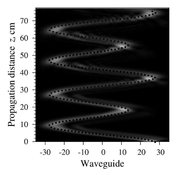
Figure 2: $\theta=50^{\circ}$

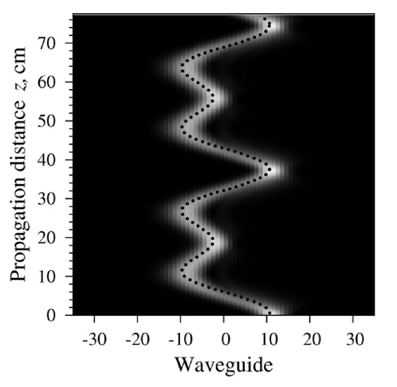
Figure 3: $\theta=60^{\circ}$

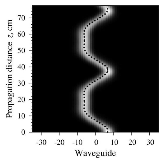
Figure 4: $\theta=70^{\circ}$

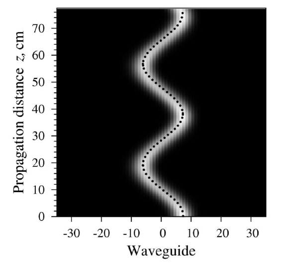
Figure 5: $\theta=180^{\circ}$

Every of these figures contains a dotted curve representing the trajectory calculated by means of the coupled modes model. The parameter $\alpha$ is found with the help of Eq. (24). The coupling constants $\gamma_{1}$ and $\gamma_{2}$ for all the values $\theta$ are calculated by the use of Eq. (28). The values $\alpha$ and $\gamma_{1}$ do not depend on $\theta$ and they are the same for all the four Figs. 2 – 5: $\alpha=16.48\leavevmode\nobreak\ \mathrm{m}^{-1}$, $\gamma_{1}=-58.44\leavevmode\nobreak\ \mathrm{m}^{-1}$. But $\gamma_{2}$ depends on the distance $b$ between the second neighbors, so $\gamma_{2}$ decreases with increasing $\theta$: $\gamma_{2}(50^{\circ})=-196.63\leavevmode\nobreak\ \mathrm{m}^{-1}$, $\gamma_{2}(60^{\circ})=-58.44\leavevmode\nobreak\ \mathrm{m}^{-1}$, $\gamma_{2}(70^{\circ})=-18.64\leavevmode\nobreak\ \mathrm{m}^{-1}$, $\gamma_{2}(180^{\circ})=-0.0277\leavevmode\nobreak\ \mathrm{m}^{-1}$. The dependence of the relation $\gamma_{2}/\gamma_{1}$ on the angle $\theta$ is depicted in Fig. 6.

Note that for $\theta=60^{\circ}$ one has $\gamma_{2}=\gamma_{1}$. This is quite expected result, since for this case $b=a$. Finely, note that for $\theta=180^{\circ}$ one has $\gamma_{2}/\gamma_{1}\sim 10^{-4}$. Thus, we confirm that for the plane array of waveguides one can neglect the SOC.

Figure 6: The dependence of the relation $\gamma_{2}/\gamma_{1}$ on the angle $\theta$.

IV Conclusion

In this paper we investigated the anharmonic Bloch oscillations in the zigzag array of the optical waveguides. For this purpose we applied the muliple scattering formalism based on the macroscopic electrodynamics approach. For the simplicity, we used the zero-harmonic approximation taking into account the TM-modes only. On the basis of the MSF, we developed the numerical algorithm for calculating the optical beam path for the specified boundary conditions at $z=0$. We chose the boundary conditions possessing the form of the Gaussian wave packet. It was shown that for this case the optical beam path takes the complicated periodic form.

This result is compared with the optical beam path predicted by means of the coupled modes model with the second-order coupling taken into account. This model contains some parameters, namely, namely, the difference between the propagation constants of the adjacent waveguides $\alpha=\beta^{(0)}_{j}-\beta^{(0)}_{j-1}$ and the coupling constants $\gamma_{1}$ and $\gamma_{2}$ for the first-order and the second-order coupling. These parameters were calculated by means of MSF. We showed that the results of calculations by two different methods are exactly the same.

Besides, we investigated the dependence of the coupling constant of the second-order coupling $\gamma_{2}$ on the angle $\theta$. It was shown that $\gamma_{2}$ decreases quickly as the angle $\theta$ increases. For $\theta=180^{\circ}$ the value $\gamma_{2}$ becomes negligible. This result confirms that for the plane array it is possible to produce the calculations taking into account the next neighbors coupling only.

Acknowledgments

The study is supported by the Russian Fund for Basic Research (Grants 13-02-00472a and 14-29-08165) and by the Ministry of Education and Science of Russian Federation, project 8364.

References

• (1) Stefano Longhi. Quantum-optical analogies using photonic structures. Laser & Photon. Rev. 3, 243 (2009).
• (2) U. Peschel, T. Pertsch, F. Lederer. Optical Bloch oscillations in waveguide arrays. Opt. Lett. 23, 1701 (1998).
• (3) T. Pertsch, P. Dannberg, W. Elflein, and A. Bräuer, F. Lederer. Optical Bloch oscillations in temperature tuned waveguide arrays. Phys. Rev. Lett. 83, 4752 (1999).
• (4) R. Morandotti, U. Peschel, J. S. Aitchison, H. S. Eisenberg, Y. Silberberg. Experimental observation of linear and nonlinear optical Bloch oscillations. Phys. Rev. Lett. 83, 4756 (1999).
• (5) T. Pertsch, T. Zentgraf, U. Peschel, A. Bräuer, F. Lederer. Beam steering in waveguide arrays. Appl. Phys. Lett. 80, 3247 (2002).
• (6) N. Chiodo, G. Della Valle, R. Osellame, S. Longhi, G. Cerullo, R. Ramponi, P. Laporta, U. Morgner. Imaging of Bloch oscillations in erbium-doped curved waveguide arrays. Opt. Lett. 31, 1651 (2006).
• (7) Zheng M. J., Xiao J. J., Yu K. W. Controllable optical Bloch oscillation in planar graded optical waveguide arrays. Phys. Rev. A 81, 033829 (2010).
• (8) H. Trompeter, T. Pertsch, F. Lederer, D. Michaelis, U. Streppel, A. Bräuer, U. Peschel Visual Observation of Zener Tunneling. Phys. Rev. Lett. 96, 023901 (2006).
• (9) F. Dreisow, A. Szameit, M. Heinrich, T. Pertsch, S. Nolte, A. Tünnermann, S. Longhi. Bloch-Zener Oscillations in Binary Superlattices. Phys. Rev. Lett. 102, 076802 (2009).
• (10) Ming Jie Zheng, Gang Wang, Kin Wah Yu. Tunable hybridization at midzone and anomalous Bloch–Zener oscillations in optical waveguide ladders. Opt. Lett. 35, 3865 (2010).
• (11) T. Schwartz, S. Fishman, M. Segev. Localisation of light in disordered lattices. Electron. Lett. 44, 165 (2008).
• (12) Y. Lahini, A. Avidan, F. Pozzi, M. Sorel, R. Morandotti, D. N. Christodoulides, Y. Silberberg. Anderson Localization and Nonlinearity in One-Dimensional Disordered Photonic Lattices. Phys. Rev. Lett. 100, 013906 (2008).
• (13) I. L. Garanovich, A. Szameit, A. A. Sukhorukov, T. Pertsch, W. Krolikowski, S. Nolte, D. Neshev, A. Tünnermann, Y. S. Kivshar. Diffraction control in periodically curved two-dimensional waveguide arrays. Optics Express 15, 9737 (2007).
• (14) F. Dreisow, M. Heinrich, A. Szameit, S. Döring, S. Nolte, A. Tünnermann, S. Fahr, F. Lederer. Spectral resolved dynamic localization in curved fs laser written waveguide arrays. Optics Express 16, 3474 (2008).
• (15) J. Joannopoulos, P. R. Villeneuve, S. Fan. Photonic crystals: putting a new twist on light. Nature 386, 143 (1997)
• (16) Busch K, Lölkes S, Wehrspohn R B, Föll H (Eds.) 2004Photonic Crystals. Advances in Design, Fabrication, and Characterization Wiley-VCH Verlag GmbH & Co. KGaA
• (17) F. Dreisow, A. Szameit, M. Heinrich, T. Pertsch, S. Nolte, A. Tünnermann. Second-order coupling in femtosecond-laser-written waveguide arrays. Optics Letters 33, 2689 (2008).
• (18) N. K. Efremidis, D. N. Christodoulides. Discrete solitons in nonlinear zigzag optical waveguide arrays with tailored diffraction properties. Phys. Rev. E 65, 056607 (2002).
• (19) A. Szameit, R. Keil, F. Dreisow, M. Heinrich, T. Pertsch, S. Nolte, A. Tünnermann. Observation of the discrete solitons in lattices with second-order interaction. Optics Letters 34, 2838 (2009).
• (20) Gang Wang, Ji Ping Huang, Kin Wah Yu. Nontrivial Bloch oscillations in waveguide arrays with second-order coupling. Optics Letters 35, 1908 (2010).
• (21) F. Dreisow, Gang Wang, M. Heinrich, R. Keil, A. Tünnermann, S. Nolte, A. Szameit. Observation of anharmonic Bloch oscillations. Optics Letters 36, 3963 (2011).
• (22) M. I. Gozman, Yu. I. Polishchuk, I. Ya. Polishchuk. On the theory of the optical Bloch oscillations. Optical Engineering 53, 071806 (2014).
• (23) M. I. Gozman, I. Ya. Polishchuk. Bloch oscillations in the optical waveguide array. arXiv:1310.5312 [cond-mat.mes-hall] (2013)
• (24) H. C. van de Hulst. Light scattering by small particles. Dover Publications, Inc. New York, 1981
• (25) M. Abramowitz and I. Stegun. Handbook of Mathematical Functions. Dover Publications, New York, 1970
• (26) A. Arriola, S. Gross, N. Jovanovic, N. Charles, P. G. Tuthill, S. M. Olaizola, A. Fuerbach, M. J. Withford. Low bend loss waveguides enable compact, efficient 3D photonic chips. Optics Express 21, 2978 (2013).
• (27) G. Palmer, S. Gross, A. Fuerbach, D. G. Lancaster, M. J. Withford. High slope efficiency and high refractive index change in direct-written Yb-doped waveguide lasers with depressed claddings. Optics Express 21, 17413 (2103).