Magnetic oscillations in a holographic liquid

Abstract

We present a holographic perspective on magnetic oscillations in strongly correlated electron systems via a fluid of charged spin 1/2 particles outside a black brane in an asymptotically anti-de-Sitter spacetime. The resulting back-reaction on the spacetime geometry and bulk gauge field gives rise to magnetic oscillations in the dual field theory, which can be directly studied without introducing probe fermions, and which differ from those predicted by Fermi liquid theory.

Introduction:

The de Haas – van Alphen effect de Haas and van Alphen (1930) refers to quantum oscillations in the magnetization as a function of $1/B$, present in metals at low temperature $T$ and strong magnetic field $B$. This phenomenon is generally associated with the Fermi surface and the observed oscillations are usually interpreted in terms of Fermi liquid theory and quasi-particles Lifshitz and Kosevich (1956). The measurement of quantum oscillations is a standard tool for investigating the electronic structure of metallic systems and this extends to strange metallic phases, where fermion excitations are strongly correlated and the quasi-particle description breaks down. The observation of quantum oscillations, in combination with ARPES experiments, leads to the conclusion that low temperature physics in such systems is still governed by a Fermi surface, although the underlying physics is not fully understood, see e.g. Sebastian et al. (2012, 2011), and may not conform to the standard Fermi liquid picture. In this paper, we provide a novel view of quantum oscillations that is not tied to a quasi-particle description but is instead based on a holographic representation of the strongly correlated electron system in terms of a dual gravitational model.

In recent years, gauge/gravity duality Maldacena (1998); Gubser et al. (1998); Witten (1998), has been applied to model strongly coupled dynamics in various condensed matter systems including strange metals (for reviews see e.g. Hartnoll (2011); Sachdev (2012)). Holographic systems at finite charge density exhibit interesting non-Fermi liquid behavior, revealed for instance in spectral functions of probe fermions Liu et al. (2011); Čubrović et al. (2009). Here we develop a simple holographic model for strongly correlated fermions in a magnetic field and use it to study magnetic oscillations in an unconventional setting. The model involves a fluid of charged spin 1/2 particles outside a dyonic black brane in 3+1 dimensional anti-de Sitter (AdS) spacetime. It takes into account the back-reaction due to charged bulk matter on the spacetime geometry and the bulk gauge field and thus extends the so-called electron star model Hartnoll et al. (2010); Hartnoll and Tavanfar (2011) to include a magnetic field and finite temperature. We obtain oscillations in the magnetization directly from the bulk gravitational physics by incorporating Landau quantization into the charged fluid description. The method differs conceptually from earlier probe fermion computations of magnetic oscillations in an electron star background Gubankova et al. (2011); Hartnoll et al. (2011a) and it predicts a dependence on the magnetic field and temperature of the oscillation amplitude that departs from Fermi liquid theory.

The Model:

Our approach is based on an extension of the electron star geometry, developed in Hartnoll et al. (2010); Hartnoll and Tavanfar (2011); Puletti et al. (2011); Hartnoll and Petrov (2011). For related work see also de Boer et al. (2010); Arsiwalla et al. (2011). This geometry is obtained by coupling Einstein – Maxwell theory to a charged perfect fluid, of non-interacting fermions of mass $m$ and charge normalized to one in units of the Maxwell coupling constant $e$,

$$S = \frac{1}{2\kappa^{2}}\int d^{4}x\sqrt{-g}\left(R-2\Lambda\right)$$ (1)

$$\;-\frac{1}{4e^{2}}\int d^{4}x\sqrt{-g}F_{\mu\nu}F^{\mu\nu}-\int d^{4}x\sqrt{-g}\,\mathcal{L}_{\rm fl}\,,\qquad$$

where $\kappa^{2}=8\pi G_{N}$ is the gravitational coupling, the AdS length scale $L$ is given in terms of the negative cosmological constant $\Lambda=-3/L^{2}$, and $\kappa/L\ll 1$ corresponds to the classical gravity (large $N$) regime. The bulk fermions are treated in a Thomas – Fermi approximation, valid for model parameters satisfying

$$mL\gg 1\,,\qquad e^{2}\sim\frac{\kappa}{L}\ll 1\,.$$ (2)

In Allais and McGreevy (2013); Medvedyeva et al. (2013) more refined computations involving holographic Fermi systems confirmed that the electron star qualitatively reproduces essential features of these models, even beyond its a priori regime of validity defined by equation (2).

Previous work on magnetic effects in holographic metals Denef et al. (2009); Hartnoll and Hofman (2010); Hartnoll et al. (2011b); Gubankova et al. (2011); Blake et al. (2012); Albash et al. (2013); Gubankova et al. (2013) has not taken into account the full back-reaction on the geometry due to the presence of charged matter in a non-vanishing magnetic field at finite temperature. The semi-classical approximation used in the electron star construction, suitably generalized to finite $B$ and $T$, also allows the back-reaction to be included in the $B\gg T$ regime, which is of primary interest to the study of magnetic oscillations. Including the back-reaction provides direct access to the underlying strong coupling dynamics without having to introduce probe fermions.

We work in a 3+1 dimensional spacetime with local coordinates $(t,x,y,r)$, which asymptotes to $\mbox{AdS}_{4}$ and which is static, stationary and has translational symmetry orthogonal to the radial direction. At any given point in the spacetime the fluid is at rest in a local Lorentz frame $e^{A}_{\mu}$, and the fluid velocity is given by $u^{\mu}=e_{0}^{\mu}$. The state of the charged fluid is completely determined by a local chemical potential and magnetic field,

$$\mu_{\rm loc}=A_{\mu}u^{\mu}\;,\qquad H_{\rm loc}=\,e^{[\mu}_{1}e^{\nu]}_{2}F_{\mu\nu}\;,\quad$$ (3)

where $A_{\mu}$ is a $U(1)$ gauge potential, and $F_{\mu\nu}$ the corresponding field strength tensor. This means that the charge density $\sigma$, the pressure $p$, and the magnetization density $\eta$ of the fluid depend only on $\mu_{\rm loc}$ and $H_{\rm loc}$. An equation of state for the fluid is obtained as in Hartnoll and Tavanfar (2011), except now the constituent dispersion relation is that of Dirac fermions in a magnetic field,

$$E_{\ell}^{2}=m^{2}+k^{2}+\big{(}2\ell+1\big{)}\gamma H_{\rm loc}\pm\gamma H_{\rm loc}\,,$$ (4)

where $\gamma$ is a constant proportional to the gyromagnetic ratio of the fermions. The index $\ell\geq 0$ labels Landau levels and the the last term on the right hand side is due to Zeeman splitting. Assuming $1/N$ effects due to bulk thermalization can be neglected Puletti et al. (2011); Hartnoll and Petrov (2011), the local pressure, charge and magnetization of the fluid are then obtained by filling states up to the Fermi level given by $\mu_{\rm loc}$. The number of occupied Landau levels is thus a local quantity,

$$\ell_{\rm filled}=\left\lfloor\frac{\mu_{\rm loc}^{2}-m^{2}}{2\gamma H_{\rm loc}}\right\rfloor\,,$$ (5)

which is determined by the equations of motion and varies with radial position in the bulk geometries of interest. In particular, there is no fluid in regions where $\ell_{\rm filled}<0$.

The field variables only depend on the radial coordinate $r$ and we choose the following parameterization for the metric,

$$ds^{2}=\frac{L^{2}}{r^{2}}\left(-\frac{\hat{c}(r)^{2}}{\hat{g}(r)^{2}}dt^{2}+dx^{2}+dy^{2}+\hat{g}(r)^{2}dr^{2}\right)\,,$$ (6)

and non-zero components of the gauge potential,

$$A_{t}=\frac{eL}{\kappa}\frac{\hat{c}(r)\hat{a}(r)}{r\hat{g}(r)}\;,\qquad A_{y}=\frac{eL}{\kappa}\hat{B}x\;.$$ (7)

This conveniently leads to simple expressions for the local chemical potential and magnetic field,

$$\mu_{\rm loc}(r)=\frac{e}{\kappa}\hat{a}(r)\,,\qquad H_{\rm loc}(r)=\frac{e}{\kappa L}\hat{B}r^{2}\,.$$ (8)

Inserting this ansatz into the Einstein-Maxwell field equations coupled to a charged fluid leads to a system of ODE’s for $\left\{\hat{a}(r),\hat{c}(r),\hat{g}(r)\right\}$, which can be solved by numerical methods along the lines of Puletti et al. (2011). The numerical algorithm is implemented on dimensionless field variables, denoted by a hat, obtained from their dimensionful counterparts by absorbing appropriate powers of $\kappa$, $e$, and $L$. For more detail, we refer to the Appendix.

The local chemical potential $\mu_{\rm loc}$ vanishes both at the horizon, $r=1$, and at the AdS boundary, $r=0$. It follows that $\ell_{\rm filled}$ can only be positive inside a finite range $r_{i}>r>r_{e}$, defining the radial region where the fluid is supported. The region between the horizon and the inner edge of the fluid $1>r>r_{i}$ is described by a vacuum dyonic black brane solution. We also have a vacuum solution in the region outside the fluid $r_{e}>r>0$, but with different black brane parameters due to the additional mass and charge of the intervening fluid. The magnetic field is the same in all three regions as the fluid particles do not carry magnetic charge, but the bulk magnetization varies due to the presence of the fluid.

A typical profile for the fluid charge density $\hat{\sigma}$ is shown in fig. 1.

Figure 1: Profile of the fluid charge density $\hat{\sigma}$, with parameters chosen so that $\max\ell_{\rm filled}=5$.

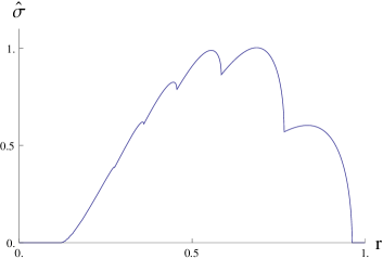
The fluid does not extend all the way to the horizon or the boundary and the bump-like shape of the profile reveals the presence of jumps in the local number of filled levels.

The AdS/CFT dictionary relates thermodynamic quantities of the dual field theory to properties of the bulk metric and gauge field. Temperature $\hat{\mathcal{T}}$ and entropy $\hat{\mathcal{S}}$ in the dual field theory are given by the Hawking temperature and entropy of the black brane, while the energy $\hat{\mathcal{E}}$, chemical potential $\hat{\mu}$, charge $\hat{\mathcal{Q}}$, magnetic field strength $\hat{\mathcal{B}}$ and magnetization $\hat{\mathcal{M}}$ of the boundary dual are read off from the asymptotic behavior of the bulk fields. The free energy follows from evaluating the on-shell action, and is found to satisfy the standard thermodynamic relation,

$$\hat{\mathcal{F}} = \hat{\mathcal{E}}-\hat{\mathcal{S}}\hat{\mathcal{T}}-\hat{\mu}\hat{\mathcal{Q}}\;.$$ (9)

The field equations of the bulk theory give rise to the following equation of state for the dual theory (see Appendix for details),

$$\frac{3}{2}\hat{\mathcal{E}} = \hat{\mathcal{S}}\hat{\mathcal{T}}+\hat{\mu}\hat{\mathcal{Q}}-\hat{\mathcal{M}}\hat{\mathcal{B}}\;,$$ (10)

which agrees with the corresponding relation for dyonic black branes in $AdS_{4}$.

Results:

The electron fluid solution is only found for restricted values of $\hat{\mathcal{B}}$ and $\hat{\mathcal{T}}$. In the absence of a magnetic field it was already observed in Puletti et al. (2011); Hartnoll and Petrov (2011), that there is a critical temperature $\hat{\mathcal{T}}_{c}$ above which there is no electron fluid and a phase transition to a vacuum black brane configuration occurs. A non-zero magnetic field brings two new aspects. First of all, the transition temperature goes down monotonically as $\hat{\mathcal{B}}$ is increased until it reaches zero at a critical magnetic field $\hat{\mathcal{B}}_{c}$, above which no electron fluid is supported at any temperature. This is evident from our numerical solutions, but can also be inferred from the analytic dyonic black brane solution (provided in the Appendix). Raising either $\hat{\mathcal{B}}$ or $\hat{\mathcal{T}}$ lowers the maximum value reached by the local chemical potential $\mu_{\rm loc}$ as a function of $r$ in the dyonic black brane background. For sufficiently high $\hat{\mathcal{B}}$ and/or $\hat{\mathcal{T}}$ the number of occupied levels $\ell_{\rm filled}$ in (5) will be nowhere positive so that no fluid can be supported and the vacuum dyonic black brane is the only available solution.

Second, the order of the phase transition changes. Whereas in Puletti et al. (2011); Hartnoll and Petrov (2011) it was found to be of third order, it becomes second order in the presence of a magnetic field. This can be shown by a similar analytic argument as was used in Hartnoll and Petrov (2011) for the $\hat{\mathcal{B}}=0$ case. Consider a temperature just below the transition temperature at $\hat{\mathcal{B}}\neq 0$, keeping the magnetic field fixed. The condition $\hat{\mu}_{\rm loc}>\hat{m}$ is then satisfied in a narrow band in the radial direction in the dyonic black brane solution and inside this band the fermions can occupy the lowest Landau level only. Furthermore, the back-reaction on the geometry due to the fermion fluid can be neglected at temperatures very close to the transition. In the presence of the fermion fluid the free energy of the system is lowered by an amount given by the on-shell action of the fluid, i.e. the integral of the fluid pressure. Near the phase transition the pressure, given by equation (20) in the Appendix, scales as $\hat{p}\propto(\hat{\mu}-\hat{m})^{3/2}$. A short calculation along the lines of Hartnoll and Petrov (2011) then results in a free energy difference, $\Delta\hat{\mathcal{F}}\propto(\hat{\mathcal{T}}_{c}-\hat{\mathcal{T}})^{2}$, between the solution with a fluid and a vacuum dyonic black brane, indicating a second order phase transition. The same behavior is also seen in our numerical solutions of the field equations with the full back-reaction included. In the limit of vanishing magnetic field, the different Landau levels collapse to a continuum and one obtains a softer dependence, $\hat{p}\propto(\hat{\mu}-\hat{m})^{5/2}$, that leads to a third order phase transition as was found in Hartnoll and Petrov (2011).

At non-vanishing magnetic field one can also approach the phase transition by varying $\hat{B}$ at fixed temperature. In this case we find $\Delta\hat{\mathcal{F}}\propto(\hat{\mathcal{B}}_{c}-\hat{\mathcal{B}})^{2}$ and the phase transition is again of second order. We anticipate that going beyond the Thomas – Fermi approximation will change the nature of the phase transition. Indeed, a first order phase transition was found at $\hat{\mathcal{B}}=0$ using WBK wave functions for the fermions in Medvedyeva et al. (2013) and we expect this would be the case at finite $\hat{\mathcal{B}}$ as well.

Figure 2: Phase diagram of dyonic electron fluid solutions for $\hat{m}=0.5$, with axes normalized such that the boundary chemical potential is $\hat{\mu}=1$. The different color shadings mark parameter regions with different maximum numbers of occupied Landau levels, increasing from left to right. In the limit $\hat{\mathcal{B}}\to 0$ the edges between the regions all asymptote to $\hat{\mathcal{T}}_{c}$, the maximal temperature at which the electron fluid is supported at $\hat{\mathcal{B}}=0$.

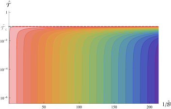
The $\hat{\mathcal{B}}-\hat{\mathcal{T}}$ phase diagram reveals a periodic feature in $1/\hat{\mathcal{B}}$. A representative plot for $\hat{m}=0.5$ is displayed in fig. 2. Changing the value of $\hat{m}$ in the numerical calculations does not significantly affect the phase diagram, apart from changing the critical values on the axes. Different colors mark different values of the maximum value of filled Landau levels $\ell_{\rm filled}$, which increases from left to right. At low temperatures the edges between regions with a different number of occupied levels occur at equal intervals in $1/\hat{\mathcal{B}}$. This periodic feature is even more apparent in the plots showing the magnetization $\hat{\mathcal{M}}$ as a function of $\hat{\mathcal{B}}$ in fig. 3. For temperatures close to the critical transition temperature $\hat{\mathcal{T}}_{c}$, the magnetization differs only slightly from that of a dyonic black brane at the same temperature and magnetic field strength but when the temperature is lowered the magnetization oscillates. The oscillations are clearly visible when $\hat{\mathcal{B}}\gg\hat{\mathcal{T}}$, which is the regime where the de Haas – van Alphen effect is observed experimentally.

Figure 3: Magnetization vs. magnetic field strength for various values of $\hat{m}$. Solid lines correspond to the electron fluid geometry, dashed ones to a dyonic black brane at same temperature and chemical potential. The labels denote temperatures $\hat{\mathcal{T}}/\hat{\mathcal{T}}_{c}=0.9\;(a),\,0.3\;(b),\,3\cdot 10^{-3}\;(c)$. In the leftmost plot $(b)$ was omitted due to too much visual overlap with the other curves. In the rightmost plot the relative sign of $\hat{\cal{M}}$ and $\hat{B}$ changes as a function of magnetic field, indicating a crossover from a diamagnetic to a paramagnetic state.

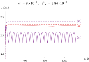
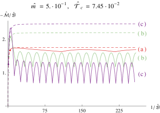
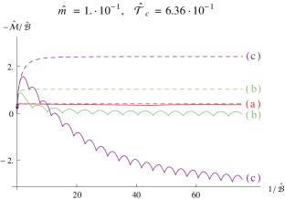
Another feature is that the magnetization of the electron fluid configuration is lower than that of a dyonic black brane with the same parameters. This is more pronounced as the value of $\hat{m}$ is lowered and when $\hat{m}$ becomes small enough, the state crosses over from diamagnetic to paramagnetic. The local magnetization is the sum of two contributions, a diamagnetic one which originates from the black brane and a paramagnetic one due to the fluid which is a gas of free electrons at zero temperature. Varying the parameter $\hat{m}$ tunes the gravitational attraction between the black brane in the center and the electron fluid surrounding it. The weaker the interaction, the larger the fluid region can grow and the more dominant the paramagnetism becomes.

For small values of the magnetic field, the overall amplitude of the magnetization is linear in $\hat{\mathcal{B}}$, as can be seen in fig. 3. This differs from the behavior predicted by the Landau theory of Fermi liquids via the Kosevich – Lifshitz formula Lifshitz and Kosevich (1956); Onsager (1952). It also differs from earlier holographic results obtained in a probe limit in Hartnoll et al. (2011b); Blake et al. (2012) and appears to be due to the gravitational back-reaction which is included in our model.

Figure 4: Period of the de Haas – van Alphen oscillations as a function of temperature for $\hat{m}=0.5$, the dotted vertical line marks the critical temperature where the solution makes the transition to a dyonic black brane.

The plots in figure 3 do not show any overlap of oscillations with different periods, suggesting that a single Fermi surface is responsible for the phenomenon. This is in agreement with Hartnoll et al. (2011b, a), where it was argued that magnetic oscillations are dominated by a single (extremal) Fermi momentum, despite the large number of holographically smeared Fermi surfaces in this system, which turn into a continuum in the Thomas – Fermi limit.

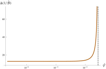
Figure 4 shows the period in $1/{\hat{\mathcal{B}}}$ of the quantum oscillations vs. temperature. It reveals a similar trend as is observed in experiments, where the period is constant at low temperature but increases with rising $T$ until the oscillations get washed out at higher temperatures. Our numerical results suggest that the oscillation period diverges in the holographic model at the critical temperature for the transition to the dyonic black brane, above which the electron fluid is no longer supported.

Discussion:

We have presented a holographic model for a 2+1 dimensional system of strongly correlated electrons in a magnetic field, involving 3+1 dimensional fermions treated in a Thomas – Fermi approximation in an asymptotically AdS dyonic black brane background, taking into account both the gravitational and electromagnetic back-reaction due to the charged matter. The system exhibits de Haas – van Alphen oscillations that appear to be dominated by a single sharp Fermi surface, while the oscillation amplitude has a non-Fermi liquid character that departs from earlier probe fermion computations.

While the semi-classical model studied here provides a relatively simple framework for numerical computations, it is rather crude. A Thomas – Fermi treatment of bulk fermions is known to wash out some quantum features that are present in more realistic models Puletti et al. (2012); Hartnoll et al. (2011a) and the sharp edges of the fluid profile for individual Landau levels can introduce fictitious non-analyticities into observables that involve derivatives acting on the bulk fields Hartnoll and Petrov (2011). The latter problem can presumably be remedied by introducing thermal effects in the bulk fluid or by replacing the anisotropic electron star by a quantum many-body model based on WKB wave functions for bulk Landau levels, along the lines of Medvedyeva et al. (2013), where the tails of the fermion wave functions naturally smooth out the edges found in the fluid description, but we leave this for future work.

.1 Appendix

Field equations:

We adapt the electron star construction developed in Hartnoll et al. (2010); Hartnoll and Tavanfar (2011); Puletti et al. (2011); Hartnoll and Petrov (2011) to include the effects of a background magnetic field. Our starting point is the action (1) in the main text, which describes a charged fluid coupled to Einstein – Maxwell theory. We will be considering static solutions describing a charged fluid suspended above the horizon of a planar dyonic black brane in 3+1 dimensional asymptotically AdS spacetime with radial electric and magnetic fields and translation symmetry in the two transverse directions. The field equations are given by

$$R_{\mu\nu}-\frac{1}{2}R\,g_{\mu\nu}+\Lambda\,g_{\mu\nu} = \kappa^{2}\left(T_{\mu\nu}^{\rm em}+T_{\mu\nu}^{\rm fl}+T_{\mu\nu}^{J}+T_{\mu\nu}^{M}\right)\,,$$

$$\nabla_{\nu}F^{\mu\nu} = e^{2}\left(J^{\mu}+\nabla_{\nu}M^{\mu\nu}\right)\,,$$ (11)

where $J^{\mu}$ and $M^{\mu\nu}$ are the fluid current and magnetization tensor,

$$J^{\mu}=-\frac{\delta\mathcal{L}_{\rm fl}}{\delta A_{\mu}}\,,\qquad M^{\mu\nu}=-2\,\frac{\delta\mathcal{L}_{\rm fl}}{\delta F_{\mu\nu}}\,,$$ (12)

and the stress energy tensors are given by

$$T_{\mu\nu}^{\rm em} = \frac{1}{e^{2}}\Big{(}F_{\mu\lambda}F_{\nu}^{~{}~{}\lambda}-\frac{1}{4}g_{\mu\nu}F_{\lambda\sigma}F^{\lambda\sigma}\Big{)}\,,$$

$$T_{\mu\nu}^{\rm fl} = -g_{\mu\nu}\mathcal{L}_{\rm fl}\,,$$

$$T_{\mu\nu}^{J} = -J_{(\mu}A_{\nu)}+u^{\lambda}A_{\lambda}u_{(\mu}J_{\nu)}-u^{\lambda}J_{\lambda}u_{(\mu}A_{\nu)}\,,$$

$$T_{\mu\nu}^{M} = M_{\lambda(\mu}F_{\nu)}^{~{}\lambda}+u^{\lambda}F_{\lambda}^{~{}\rho}u_{(\mu}M_{\nu)\rho}-u^{\lambda}M_{\lambda\rho}u_{(\mu}F_{\nu)}^{~{}~{}\rho}\,.~{}~{}~{}~{}~{}$$ (13)

Let $e_{\mu}^{A}$ denote a local Lorentz frame where the fluid is at rest. The fluid four velocity is then given by $u^{\mu}=e^{\mu}_{0}$ and the fluid components experience a local chemical potential and a local magnetic field,

$$\mu_{\rm loc}=A_{\mu}u^{\mu}\,,\qquad H_{\rm loc}=\,e_{\>1}^{[\mu}e_{\,2}^{\nu]}F_{\mu\nu}\,,$$ (14)

which completely determine the state of the charged fluid at a given point in the bulk spacetime. In particular, the electric current and magnetic polarization, which can be expressed in terms of local charge and magnetization densities, $J^{\mu}=\sigma u^{\mu}$, $M^{\mu\nu}=2\,\eta\,e_{\>1}^{[\mu}e_{\,2}^{\nu]}$, and the on-shell fluid Lagrangian density, given by the pressure $\mathcal{L}_{\rm fl}=-p$ for the static solutions we are considering, are all functions of $\mu_{\rm loc}$ and $H_{\rm loc}$.

The formalism we are using derives from so called spin fluid models, which have been studied in general relativity since the 1970’s Schutz (1970); Ray (1972); Bailey and Israel (1975); de Oliveira and Salim (1991); Brown (1993); de Oliveira and Salim (1995). We have only presented the minimal ingredients needed to describe the static geometries that are of interest here, but the full formalism can also handle more general dynamical backgrounds.

Fluid variables:

The bulk variables that describe the fluid are the charge density $\sigma$, the magnetization density $\eta$ and the pressure $p$. The fluid components are locally free fermions in an external magnetic field along the radial direction, with dispersion relation

$$E_{\ell}^{2}=m^{2}+k^{2}+\Big{(}2\ell+1\Big{)}\gamma H_{\rm loc}\pm\gamma H_{\rm loc}\,,$$ (15)

where the index $\ell\geq 0$ labels the Landau levels, $\gamma$ is a constant proportional to the gyromagnetic ratio of the constituent fermions, and the $\pm$ in the rightmost term is due to Zeeman splitting. There is a degeneracy between different sign Zeeman states in adjacent Landau levels. The sum over levels can therefore be rearranged into a sum $\sum^{\prime}_{\ell\geq 0}$, where the prime indicates inserting a relative factor of $1/2$ in the $\ell=0$ term. The density of states is

$$n(E) = {{\beta}\gamma}{H}_{\rm loc}{\sum_{\ell\geq 0}}^{\prime}\theta(E^{2}-\epsilon_{\ell}^{2})\frac{E}{\sqrt{E^{2}-\epsilon_{\ell}^{2}}}\,,$$ (16)

where $\beta$ is a constant and $\epsilon_{\ell}=\sqrt{m^{2}+2\,\ell\,\gamma\,H_{\mathrm{loc}}}$ is the energy in the Landau level labelled by $\ell$. In the limit of weak magnetic field the sum over Landau levels can be replaced by an integral, which is easily performed to reproduce the density of states used to construct an electron star in zero magnetic field in Hartnoll and Tavanfar (2011).

The local charge density $\sigma$ is obtained from the density of states via

$$\sigma=\int_{0}^{\mu_{\rm loc}}n(E)dE\,,$$ (17)

and the pressure and magnetization density are obtained from the charge density by the thermodynamic relations,

$$\frac{\partial p}{\partial\mu_{\rm loc}}=\sigma\,,\quad\frac{\partial p}{\partial H_{\rm loc}}=\eta\,,\qquad$$ (18)

analogous to the electron star Hartnoll and Tavanfar (2011). The constant of integration in $p$ is fixed such that $p$ vanishes for $\sigma=0$. Using the density of states in (16) leads to the following explicit expressions for the fluid variables in terms of the local chemical potential and local magnetic field,

$$\sigma = {{\beta}\gamma}{H}_{\rm loc}{\sum_{\ell\geq 0}}^{\prime}{\theta\left(\mu^{2}_{\rm loc}-\epsilon_{\ell}^{2}\right)\sqrt{\mu^{2}_{\rm loc}-\epsilon_{\ell}^{2}}}\,,$$ (19)

$$p = \frac{\gamma\beta}{2}H_{\rm loc}{\sum_{\ell\geq 0}}^{\prime}\theta\left(\mu^{2}_{\rm loc}-\epsilon_{\ell}^{2}\right)\left[\mu_{\rm loc}\sqrt{\mu_{\rm loc}^{2}-\epsilon_{\ell}^{2}}-\epsilon_{\ell}^{2}\log\left(\frac{\sqrt{\mu_{\rm loc}^{2}-\epsilon_{\ell}^{2}}+\mu_{\rm loc}}{\epsilon_{\ell}}\right)\right]\,,$$ (20)

$$\eta = \frac{\gamma\beta}{2}{\sum_{\ell\geq 0}}^{\prime}\theta\left(\mu^{2}_{\rm loc}-\epsilon_{\ell}^{2}\right)\left[\mu_{\rm loc}\sqrt{\mu_{\rm loc}^{2}-\epsilon_{\ell}^{2}}-\left(2\epsilon_{\ell}^{2}-m^{2}\right)\log\left(\frac{\sqrt{\mu_{\rm loc}^{2}-\epsilon_{\ell}^{2}}+\mu_{\rm loc}}{\epsilon_{\ell}}\right)\right]\,.$$ (21)

The matter stress-energy tensors in (13) reduce to

$$T^{\rm fl}_{\mu\nu}=p\,g_{\mu\nu}\,,\qquad T_{\mu\nu}^{J}=\mu_{\rm loc}\,\sigma\,u_{\mu}u_{\nu}\,,$$

$$T^{M}_{\mu\nu}=-\frac{1}{2}H_{\rm loc}\,\eta\,(e_{\mu}^{1}e_{\nu}^{1}+e_{\mu}^{2}e_{\nu}^{2})\,.$$ (22)

We proceed to solve the combined Einstein and Maxwell equations for this system with the above expressions for the fluid variables.

Metric and gauge field ansatz:

Parameterizing non-vanishing components of the tetrad as

$$e_{t}^{0}=\frac{L}{r}\frac{\hat{c}(r)}{\hat{g}(r)}\;,\quad e_{x}^{1}=e_{y}^{2}=\frac{L}{r}\;,\quad e_{r}^{3}=\frac{L}{r}\hat{g}(r)\;,$$ (23)

and the gauge potential as

$$A_{t}=\frac{eL}{\kappa}\frac{\hat{c}(r)\hat{a}(r)}{r\hat{g}(r)}\;,\qquad A_{y}=\frac{eL}{\kappa}\hat{B}x\;,$$ (24)

yields the following local chemical potential and magnetic field,

$$\mu_{\rm loc}(r)=\frac{e}{\kappa}\hat{a}(r)\,,\qquad H_{\rm loc}(r)=\frac{e}{\kappa L}\hat{B}r^{2}\,.$$ (25)

Hats denote dimensionless quantities and we find it useful to convert all parameters and field variables into dimensionless form Hartnoll and Tavanfar (2011),

$$\hat{m}=\frac{\kappa}{e}m\,,\quad\hat{\beta}=\frac{e^{4}L^{2}}{\kappa^{2}}\beta\,,\quad\hat{\gamma}=\frac{\kappa}{eL}\gamma\,,$$

$$\hat{\mu}_{\rm loc}=\frac{\kappa}{e}\mu_{\rm loc}\,,\quad\hat{H}_{\rm loc}=\frac{\kappa L}{e}H_{\rm loc}\,,\quad$$

$$\hat{\sigma}=e\kappa L^{2}\,\sigma\,,\quad\hat{p}=\kappa^{2}L^{2}\,p\,,\quad\hat{\eta}=e\kappa L\,\eta\,.$$ (26)

Final form of the field equations:

The Einstein and Maxwell equations (11), with stress-energy tensors given by (LABEL:def_tensors_exp) and the ansatz (23)-(24) for the metric and the Maxwell gauge field, reduce to a system of first order ordinary differential equations,

$$r\frac{d\hat{c}}{dr} = -\frac{1}{2}\hat{c}\,\hat{g}^{2}\hat{a}\,\hat{\sigma}\,,$$ (27)

$$r\frac{d\hat{g}}{dr} = -\frac{3}{2}\hat{g}-\frac{1}{4}\hat{g}^{3}(\hat{B}^{2}r^{4}{+}\hat{q}^{2}r^{4}{-}6{-}2\hat{p}+2\hat{a}\,\hat{\sigma}),$$ (28)

$$r\frac{d\hat{a}}{dr} = -\frac{\hat{a}}{2}-r^{2}\hat{g}\,\hat{q}-\frac{\hat{a}\,\hat{g}^{2}}{4}(\hat{B}^{2}r^{4}{+}\hat{q}^{2}r^{4}{-}6{-}2\hat{p}),$$ (29)

$$r\frac{d\hat{q}}{dr} = -\frac{1}{r^{2}}\,\hat{g}\,\hat{\sigma}\,,$$ (30)

$$r\,\frac{d\hat{\mathfrak{M}}}{dr} = \hat{B}\,r-\frac{\hat{\eta}}{r}+\frac{1}{2}\hat{a}\,\hat{g}^{2}\,\hat{\sigma}\,\hat{\mathfrak{M}}\,.$$ (31)

We have introduced two auxiliary functions. One is $\hat{q}(r)$, which is related to the value of the local electric field by $e_{0}^{t}e_{3}^{r}F_{tr}=\frac{e}{\kappa L}r^{2}\hat{q}$. The other is $\hat{\mathfrak{M}}$, which originates from the functional derivative $\frac{\delta S}{\delta F_{xy}}$ of the on-shell action, and whose value at $r=0$ is the magnetization in the boundary theory, $\hat{\mathcal{M}}=\lim_{r\to 0}\hat{\mathfrak{M}}(r)$. Finally, energy-momentum conservation can be expressed as

$$\frac{d\hat{p}}{dr}=\hat{\sigma}\frac{d\hat{a}}{dr}+2\,r\hat{B}\,\hat{\eta}\,.$$ (32)

The following quantity

$$\mathcal{\hat{Y}} = \hat{c}\left[\frac{3+\hat{p}}{r^{3}}-\frac{3}{r^{3}\hat{g}^{2}}-\frac{2\hat{a}\hat{q}}{r\hat{g}}+2\hat{B}\,\hat{\mathfrak{M}}-\frac{r(\hat{B}^{2}+\hat{q}^{2})}{2}\right]\;~{}~{}~{}~{}$$ (33)

is constant along the radial direction $r$ when the field equations are satisfied, and later on we use this to determine (40), the equation of state in the dual boundary field theory.

Solutions:

In the presence of a charged fluid we have to solve the field equations (27)-(31) numerically. As discussed in the main text, the fluid is only supported where the local chemical potential is larger than the minimum energy state in the lowest Landau level. In solutions with a non-vanishing fluid profile this condition is met inside a radial range $1>r_{i}>r>r_{e}>0$, where $r=1$ is the radial location of the brane horizon, and $r=0$ marks spatial infinity of the spacetime.

In the region $1>r>r_{i}$, there is no fluid and the solution of the field equations is a dyonic black brane,

$$\hat{c}(r)=1\,,\quad\frac{\hat{a}(r)}{r\hat{g}(r)}=\hat{Q}(1-r)\,,\quad$$

$$\frac{1}{\hat{g}(r)^{2}}=1-\frac{2+\hat{Q}^{2}+\hat{B}^{2}}{2}r^{3}+\frac{\hat{Q}^{2}+\hat{B}^{2}}{2}r^{4}\,.$$ (34)

The local chemical potential grows as we move outwards from the horizon and by equation (5) in the main text the lowest Landau level can be occupied if $\hat{\mu}_{\textrm{loc}}^{2}\geq\hat{m}^{2}$. The radial position $r=r_{i}$ outside the black brane horizon where this condition is first satisfied defines the inner edge of the fluid. The dyonic black brane solution then provides initial data at $r=r_{i}$ for the subsequent numerical evaluation of the system of equations (27)-(31) in the fluid region. At high temperature, the condition is not satisfied anywhere outside the brane horizon. In this case there will be no fluid and the only solution is the dyonic black brane itself. Whenever a solution with a fluid present exists, however, it has a lower free energy density than a dyonic black brane at the same temperature.

Returning to the description of the fluid solution, the local chemical potential reaches a maximum and then decreases towards the exterior edge $r=r_{e}$ where the fluid is no longer supported. Outside the fluid, we have another dyonic black brane solution with parameters determined by the output of the numerical integration at $r=r_{e}$,

$$\hat{c}(r) = \mathfrak{c}\,,\quad\frac{\hat{a}(r)}{r\hat{g}(r)}=\hat{\mu}-\hat{\mathcal{Q}}\,r,\quad$$

$$\frac{1}{\hat{g}(r)^{2}} = 1-\hat{\mathcal{E}}\,r^{3}+\frac{\hat{\mathcal{Q}}^{2}+\hat{\mathcal{B}}^{2}}{2}r^{4}\,,$$ (35)

with

$$\hat{\mathcal{B}} = \hat{B}\,,~{}~{}\mathfrak{c}=\hat{c}(r_{e})\,,~{}~{}\hat{\mathcal{Q}}=\hat{q}(r_{e})\,,~{}~{}\hat{\mu}=\frac{\hat{a}(r_{e})}{r_{e}\hat{g}(r_{e})}+r_{e}\hat{q}(r_{e})$$

$$\hat{\mathcal{E}} = \frac{1}{r_{e}^{3}}\left(1-\frac{1}{\hat{g}(r_{e})^{2}}\right)+\frac{r_{e}}{2}\left(\hat{B}^{2}+\hat{q}(r_{e})^{2}\right)\,.$$ (36)

Calligraphic letters denote boundary quantities and hatted calligraphic letters denote dimensionless boundary quantities. The boundary magnetization is given by the value of the auxiliary function $\hat{\mathfrak{M}}(r)$ at $r=0$, which can obtained by integrating (31) from the outer edge of the fluid to the AdS boundary,

$$\hat{\mathcal{M}}=\lim_{r\to 0}\hat{\mathfrak{M}}(r)=-\hat{B}\,r_{e}+\hat{\mathfrak{M}}(r_{e})\,.$$ (37)

Thermodynamics:

The dual field theory temperature and entropy are the Hawking temperature and Bekenstein-Hawking entropy of the black brane. Restoring dimensions to our quantities, we obtain

$${\mathcal{T}}=\frac{1}{8\pi\mathfrak{c}L}\left(6-\hat{Q}^{2}-\hat{B}^{2}\right)\,,\qquad{\mathcal{S}}=\frac{2\pi}{\kappa^{2}}V_{2}\,,~{}~{}~{}~{}~{}~{}$$ (38)

where the $\mathfrak{c}$ keeps track of the different time normalization at the inner and outer edges of the fluid and $V_{2}$ is the volume of the two-dimensional boundary. The free energy is computed from the on-shell regularized Euclidean action,

$$\mathcal{F}=\mathcal{E}-\mathcal{S}\mathcal{T}-\mu\mathcal{Q}\,.$$ (39)

Evaluating the conserved charge $\mathcal{Y}$ (33) at the horizon of (33), and at the boundary (.1) gives the thermodynamic relation

$$\frac{3}{2}\mathcal{E}=\mathcal{S}\mathcal{T}+\mu\mathcal{Q}-\mathcal{M}\mathcal{B}\,,~{}~{}~{}$$ (40)

once we restore dimensions according to

$$\mathcal{E}=\frac{V_{2}}{\kappa^{2}\,L}\hat{\mathcal{E}}\,,~{}~{}~{}\mu=\frac{eL}{\kappa}\,\hat{\mu}\,,~{}~{}~{}\mathcal{Q}=\frac{V_{2}}{\kappa eL^{2}}\hat{\mathcal{Q}}\,,$$

$$\mathcal{B}=\frac{eL}{\kappa}\,\hat{\mathcal{B}}\,,~{}~{}~{}\mathcal{M}=\frac{V_{2}}{\kappa eL^{2}}\hat{\mathcal{M}}\,.$$ (41)

References

- de Haas and van Alphen (1930) W. J. de Haas and P. M. van Alphen, Communications from the Physical Laboratory of the University of Leiden 208d,212a (1930).
- Lifshitz and Kosevich (1956) L. Lifshitz and A. M. Kosevich, Zh. Éksp. Teor. Fiz. [Sov. Phys. JETP 2, 636 (1956)] 29, 730 (1956).
- Sebastian et al. (2012) S. E. Sebastian, N. Harrison, and G. G. Lonzarich, Reports on Progress in Physics 75, 102501 (2012).
- Sebastian et al. (2011) S. E. Sebastian, N. Harrison, and G. G. Lonzarich, 369, 1687 (2011).
- Maldacena (1998) J. M. Maldacena, Adv. Theor. Math. Phys. 2, 231 (1998), arXiv:hep-th/9711200 .
- Gubser et al. (1998) S. S. Gubser, I. R. Klebanov, and A. M. Polyakov, Phys. Lett. B428, 105 (1998), arXiv:hep-th/9802109 .
- Witten (1998) E. Witten, Adv. Theor. Math. Phys. 2, 253 (1998), arXiv:hep-th/9802150 .
- Hartnoll (2011) S. A. Hartnoll, (2011), arXiv:1106.4324 [hep-th] .
- Sachdev (2012) S. Sachdev, Ann.Rev.Condensed Matter Phys. 3, 9 (2012), arXiv:1108.1197 [cond-mat.str-el] .
- Liu et al. (2011) H. Liu, J. McGreevy, and D. Vegh, Phys.Rev. D83, 065029 (2011), arXiv:0903.2477 [hep-th] .
- Čubrović et al. (2009) M. Čubrović, J. Zaanen, and K. Schalm, Science 325, 439 (2009), arXiv:0904.1993 [hep-th] .
- Hartnoll et al. (2010) S. A. Hartnoll, J. Polchinski, E. Silverstein, and D. Tong, JHEP 1004, 120 (2010), arXiv:0912.1061 [hep-th] .
- Hartnoll and Tavanfar (2011) S. A. Hartnoll and A. Tavanfar, Phys.Rev. D83, 046003 (2011), arXiv:1008.2828 [hep-th] .
- Gubankova et al. (2011) E. Gubankova, J. Brill, M. Čubrović, K. Schalm, P. Schijven, et al., Phys.Rev. D84, 106003 (2011), arXiv:1011.4051 [hep-th] .
- Hartnoll et al. (2011a) S. A. Hartnoll, D. M. Hofman, and D. Vegh, JHEP 1108, 096 (2011a), arXiv:1105.3197 [hep-th] .
- Puletti et al. (2011) V. G. M. Puletti, S. Nowling, L. Thorlacius, and T. Zingg, JHEP 1101, 117 (2011), arXiv:1011.6261 [hep-th] .
- Hartnoll and Petrov (2011) S. A. Hartnoll and P. Petrov, Phys.Rev.Lett. 106, 121601 (2011), arXiv:1011.6469 [hep-th] .
- de Boer et al. (2010) J. de Boer, K. Papadodimas, and E. Verlinde, JHEP 1010, 020 (2010), arXiv:0907.2695 [hep-th] .
- Arsiwalla et al. (2011) X. Arsiwalla, J. de Boer, K. Papadodimas, and E. Verlinde, JHEP 1101, 144 (2011), arXiv:1010.5784 [hep-th] .
- Allais and McGreevy (2013) A. Allais and J. McGreevy, Phys.Rev. D88, 066006 (2013), arXiv:1306.6075 [hep-th] .
- Medvedyeva et al. (2013) M. V. Medvedyeva, E. Gubankova, M. Čubrović, K. Schalm, and J. Zaanen, JHEP 1312, 025 (2013), arXiv:1302.5149 [hep-th] .
- Denef et al. (2009) F. Denef, S. A. Hartnoll, and S. Sachdev, Phys.Rev. D80, 126016 (2009), arXiv:0908.1788 [hep-th] .
- Hartnoll and Hofman (2010) S. A. Hartnoll and D. M. Hofman, Phys.Rev. B81, 155125 (2010), arXiv:0912.0008 [cond-mat.str-el] .
- Hartnoll et al. (2011b) S. A. Hartnoll, D. M. Hofman, and A. Tavanfar, Europhys.Lett. 95, 31002 (2011b), arXiv:1011.2502 [hep-th] .
- Blake et al. (2012) M. Blake, S. Bolognesi, D. Tong, and K. Wong, JHEP 1212, 039 (2012), arXiv:1208.5771 [hep-th] .
- Albash et al. (2013) T. Albash, C. V. Johnson, and S. MacDonald, Lect.Notes Phys. 871, 537 (2013), arXiv:1207.1677 [hep-th] .
- Gubankova et al. (2013) E. Gubankova, J. Brill, M. Čubrović, K. Schalm, P. Schijven, et al., Lect.Notes Phys. 871, 555 (2013), arXiv:1304.3835 [hep-th] .
- Onsager (1952) L. Onsager, Phil. Mag. 43, 1006 (1952).
- Puletti et al. (2012) V. G. M. Puletti, S. Nowling, L. Thorlacius, and T. Zingg, JHEP 01, 073 (2012), arXiv:1110.4601 [hep-th] .
- Schutz (1970) B. F. Schutz, Physical Review D 2, 2762 (1970).
- Ray (1972) J. R. Ray, Journal of Mathematical Physics 13, 1451 (1972).
- Bailey and Israel (1975) I. Bailey and W. Israel, Communications in Mathematical Physics 42, 65 (1975).
- de Oliveira and Salim (1991) H. de Oliveira and J. Salim, Class.Quant.Grav. 8, 1199 (1991).
- Brown (1993) J. D. Brown, Class.Quant.Grav. 10, 1579 (1993), arXiv:gr-qc/9304026 [gr-qc] .
- de Oliveira and Salim (1995) H. P. de Oliveira and J. Salim, Physics Letters A 201, 381 (1995).