Generalized Formalisms of the Radio Interferometer Measurement Equation

Abstract

The Radio Interferometer Measurement Equation (RIME) is a matrix-based mathematical model that describes the response of a radio interferometer. The Jones calculus it employs is not suitable for describing the analogue components of a telescope. This is because it does not consider the effect of impedance mismatches between components. This paper aims to highlight the limitations of Jones calculus, and suggests some alternative methods that are more applicable. We reformulate the RIME with a different basis that includes magnetic and mixed coherency statistics. We present a microwave network inspired 2N-port version of the RIME, and a tensor formalism based upon the electromagnetic tensor from special relativity. We elucidate the limitations of the Jones-matrix-based RIME for describing analogue components. We show how measured scattering parameters of analogue components can be used in a 2N-port version of the RIME. In addition, we show how motion at relativistic speed affects the observed flux. We present reformulations of the RIME that correctly account for magnetic field coherency. These reformulations extend the standard formulation, highlight its limitations, and may have applications in space-based interferometry and precise absolute calibration experiments.

1 Introduction

Coherency in electromagnetic fields is a fundamental topic within optics. Its importance in fields such as radio astronomy can not be overstated: interferometry and synthesis imaging techniques rely heavily upon coherency theory (Taylor et al., 1999; Mandel & Wolf, 1995; Thompson et al., 2004). Of particular importance to radio astronomy is the Van-Cittert-Zernicke theorem (vC-Z, Zernicke, 1938) and the radio interferometer Measurement Equation (RIME, Hamaker et al., 1996). The vC-Z relates the brightness of a source to its mutual coherency as measured by an interferometer, and the RIME provides a polarimetric framework to calibrate out corruptions caused along the signal’s path.

While the vC-Z theorem dates back to 1938, more recent work such as that of Carozzi & Woan (2009) extends its applicability to polarized measurements over wide fields of view. The RIME has a much shorter history: it was not formulated until 1996 (Hamaker et al., 1996). Before the RIME, calibration was conducted in an ad-hoc manner, with each polarization essentially treated separately. The framework was expounded in a series of follow-up papers (Sault et al., 1996; Hamaker & Bregman, 1996; Hamaker, 2000, 2006); recent work by Smirnov extends the formalism to the full sky case, and reformulates the RIME using tensor algebra (Smirnov, 2011a, b).

This article introduces two reformulations of the RIME, that extend its applicability and demonstrates limitations with the Jones-matrix-based formalism. Both of these reformulations consider full electromagnetic coherency statistics (i.e. electric, magnetic and mixed coherencies). The first is inspired by transmission matrix methods from microwave engineering. We show that this reformulation better accounts for the changes in impedance between analogue components within a radio telescope. The second reformulation is a relativistic-aware formulation of the RIME, starting with the electromagnetic field tensor. This formalism allows for relativistic motion to be treated as instrumental effect and incorporated into the RIME.

This article is organized as follows. In Section 2, we review existing formalisms of the RIME and methods from microwave engineering. Section 3 defines coherency matrices, which are used in Section 4 to formulate general coherency relationships for radio astronomy. In Section 5, we introduce a tensor formulation of the RIME based upon the electromagnetic tensor from special relativity. Discussion and example applications are given in Section 6; concluding remarks are given in Section 7.

2 Jones and Mueller RIME formulations

Before continuing on to derive a more general relationship between the two-point coherency matrix and the voltage-current coherency, we would like to give a brief overview and derivation of the radio interferometer Measurement Equation of Hamaker et al. (1996). Our motivation behind this is to highlight that Hamaker et. al.’s RIME is a special case of a more general (and thus less limited) coherency relationship.

In their seminal Measurement Equation (ME) paper, Hamaker et al. (1996) showed that Mueller and Jones calculuses provide a good framework for modelling radio interferometers. In optics, Jones and Mueller matrices are used to model the transmission of light through optical elements (Jones, 1941; Mueller, 1948). Mueller matrices are $\mbox{4}\times\mbox{4}$ matrices that act upon the Stokes vector

$$\mbox{{\emph{s}}}=\begin{pmatrix}I&Q&U&V\end{pmatrix}^{T},$$ (1)

whereas Jones matrices are only $\mbox{2}\times\mbox{2}$ in dimension and act upon the ‘Jones vector’: the electric field vector in a coordinate system such that z-axis is aligned with the Poynting vector

$$\mbox{{\emph{e}}}(\mbox{\emph{{r}}},t)=\begin{pmatrix}e_{x}(\mbox{\emph{{r}}},t)&e_{y}(\mbox{\emph{{r}}},t)\end{pmatrix}^{T}.$$ (2)

Jones calculus dictates that along a signal’s path, any (linear) transformation can be represented with a Jones matrix, J:

$$\mbox{{\emph{e}}}_{\rm{out}}(\mbox{{\emph{r}}},t)=\mbox{{\emph{J}}}\mbox{{\emph{e}}}_{\rm{in}}(\mbox{{\emph{r}}},t)$$ (3)

A useful property of Jones calculus is that multiple effects along a signal’s path of propagation correspond to repeated multiplications:

$$\mbox{{\emph{e}}}_{\mathrm{out}}(\mbox{{\emph{r}}},t)=\emph{{J}}_{n}\cdots\emph{{J}}_{2}\emph{{J}}_{1}\mbox{{\emph{e}}}_{\rm{in}}(\mbox{{\emph{r}}},t),$$ (4)

which can be collapsed into a single matrix when required.

The RIME uses Jones matrices to model the various corruptions and effects during a signal’s journey from a source right though to the correlator. A block diagram for a (simplified) two-element interferometer is shown in Figure 1. From left to right, the figure shows the journey of a signal from a source right through to the correlator. The radiation from the source is picked up by two antennas, which we have denoted with subscript $p$ and $q$. The radiation follows a unique path to both of these antennas; each antenna also has associated with it a unique chain of analogue components that amplify and filter the signal to prepare it for correlation. Each of these subscripted boxes may be represented by a Jones matrix; alternatively an overall Jones matrix can be formed for the $p$ and $q$ branches (the dashed areas).

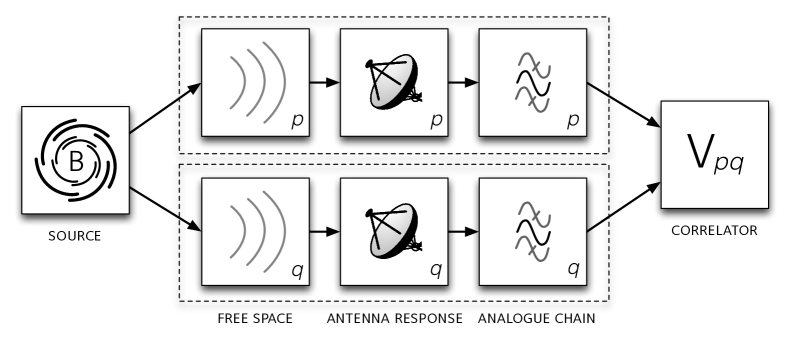
Figure 1: Block diagram showing a simple model of an interferometer that can be modelled with the RIME. Radiation from a source propagates through free space to two telescopes, p and q. After passing through the telescope’s analogue chain, the two signals are interfered in a cross-correlator.

2.1 Hamaker’s RIME derivation

The derivation of the RIME is remarkably simple and elegant. For a single point source of radiation, the voltages induced at the terminals of a pair of antennas, $p$ and $q$ are

$$\mbox{{\emph{v}}}_{p}(t) =\mbox{{\emph{J}}}_{p}\mbox{{\emph{e}}}_{0}(t)$$ (5)

$$\mbox{{\emph{v}}}_{q}(t) =\mbox{{\emph{J}}}_{q}\mbox{{\emph{e}}}_{0}(t)$$ (6)

In its simplest form, the RIME is formed by taking the outer product of these two relationships. Note that in their original paper, the authors use the Kronecker incarnation of the outer product, which we will denote with $\star$. We reserve the symbol $\otimes$ for the matrix outer product of two matrices $\emph{{A}}\otimes\emph{{B}}=\mbox{{\emph{A}}}\emph{{B}}^{H},$ where H denotes the Hermitian conjugate transpose. Using the Kronecker outer product, the RIME is given by

$$\left\langle\mbox{{\emph{v}}}_{p}\star\mbox{{\emph{v}}}_{q}\right\rangle=\left(\mbox{{\emph{J}}}_{p}\star\mbox{{\emph{J}}}_{q}\right)\left\langle\mbox{{\emph{e}}}_{0}\star\mbox{{\emph{e}}}_{0}\right\rangle=\left(\mbox{{\emph{J}}}_{p}\star\mbox{{\emph{J}}}_{q}\right)\mbox{{\emph{e}}}_{00}$$ (7)

where $\mbox{{\emph{J}}}_{p}$ and $\mbox{{\emph{J}}}_{q}$ are the Jones matrices representing all transformations along the two signal paths, and $\left(\mbox{{\emph{J}}}_{p}\star\mbox{{\emph{J}}}_{q}\right)$ is a $\mbox{4}\times\mbox{4}$ matrix. Here, $\mbox{{\emph{e}}}_{00}$ is the sky brightness of a single point source of radiation. For a multi-element interferometer, every antenna has its own unique Jones matrix, and a RIME may be written for every pair of antennas.

Due to their choice of outer product, Hamaker et. al. arrive at a coherency vector

$$\mbox{{\emph{e}}}_{pq}(\mbox{{\emph{r}}}_{p},\mbox{{\emph{r}}}_{q},\tau)=\left\langle\mbox{{\emph{e}}}_{p}(\mbox{{\emph{r}}}_{p},t)\star\mbox{{\emph{e}}}_{q}(\mbox{{\emph{r}}}_{q},t+\tau)\right\rangle=\begin{pmatrix}\left\langle e_{px}e_{qx}^{*}\right\rangle\\ \left\langle e_{px}e_{qy}^{*}\right\rangle\\ \left\langle e_{py}e_{qx}^{*}\right\rangle\\ \left\langle e_{py}e_{qy}^{*}\right\rangle\end{pmatrix},$$ (8)

as opposed to the coherency matrix of Wolf (1954); this is introduced in §3.1 below. The column vector of a point source at $\mbox{{\emph{r}}}_{0}$ is then $\mbox{{\emph{e}}}_{00}$; that is, $p=q$ and $\tau=0$. The vector $\mbox{{\emph{e}}}_{00}$ is related to the Stokes vector by the transform.

$$\begin{pmatrix}I\\ Q\\ U\\ V\end{pmatrix}=\begin{pmatrix}1&0&0&1\\ 1&0&0&-1\\ 0&1&1&0\\ 0&-j&j&0\end{pmatrix}\begin{pmatrix}\left\langle e_{0x}e_{0x}^{*}\right\rangle\\ \left\langle e_{0x}e_{0y}^{*}\right\rangle\\ \left\langle e_{0y}e_{0x}^{*}\right\rangle\\ \left\langle e_{0y}e_{0y}^{*}\right\rangle\end{pmatrix}.$$ (9)

The quantity $\left(\mbox{{\emph{J}}}_{p}\star\mbox{{\emph{J}}}_{q}\right)$ in Eq. 7 can therefore be viewed as a Mueller matrix. That is, Eq. 7 can be considered a Mueller-calculus-based ME for a radio interferometer. To summarize, Hamaker et. al. showed that:

• Jones matrices can be used to model the propagation of a signal from a radiation source through to the voltage at the terminal of an antenna.

• A Mueller matrix can be formed from the Jones terms of a pair of antennas, which then relates the measured voltage coherency of that pair to a source’s brightness.

Showing that these calculuses were applicable and indeed useful for modelling and calibrating radio interferometers was an important step forward in radio polarimetry.

2.2 The 2$\times$2 RIME

In a later paper, Hamaker (2000) presents a modified formulation of the RIME, where instead of forming the coherency vector from the Kronecker outer product ($\star$), the coherency matrix is formed from the matrix outer product ($\otimes$):

$$\mbox{{\emph{E}}}_{pq}=\left\langle\emph{{e}}_{p}\otimes\emph{{e}}_{q}\right\rangle=\begin{pmatrix}\left\langle e_{px}e_{qx}^{*}\right\rangle&\left\langle e_{px}e_{qy}^{*}\right\rangle\\ \left\langle e_{px}e_{qx}^{*}\right\rangle&\left\langle e_{py}e_{qy}^{*}\right\rangle\end{pmatrix}$$ (10)

The resulting coherency matrix is then shown to be related to the Stokes parameters by $\mbox{{\emph{E}}}_{00}=\mbox{ {B} }$, where

$$\mathsf{B} =\begin{pmatrix}I+Q&U+jV\\ U-jV&I-Q\end{pmatrix}.$$ (11)

The equivalent to the RIME of Eq. 7 is

$$\left\langle\mbox{{\emph{v}}}_{p}\otimes\mbox{{\emph{v}}}_{q}\right\rangle=2\left\langle\mbox{($\mbox{{\emph{J}}}_{p}\textbf{\emph{e}}$}_{0})\otimes(\mbox{{\emph{J}}}_{q}\mbox{{\emph{e}}}_{0})\right\rangle=2\mbox{{\emph{J}}}_{p}\left\langle\mbox{{\emph{e}}}_{0}\otimes\mbox{{\emph{e}}}_{0}\right\rangle\mbox{{\emph{J}}}_{q}^{H}$$ (12)

or more simply,

$$\mathsf{V}_{pq}=\mbox{{\emph{J}}}_{p}\mbox{{\emph{B}}}\mbox{{\emph{J}}}_{q}^{H}.$$ (13)

This approach avoids the need to use $\mbox{4}\times\mbox{4}$ Mueller matrices, so is both simpler and computationally advantageous. This form is also cleaner in appearance, as fewer indices are required.

Smirnov (2011a) takes the $\mbox{2}\times\mbox{2}$ version of the RIME as a starting point and extends the RIME to a full sky case. By treating the sky as a brightness distribution $\mathsf{B}$($\sigma$), where $\sigma$ is a direction vector, each antenna has a Jones term $\mbox{{\emph{J}}}_{p}(\sigma)$ describing the signal path for a given direction. The visibility matrix $\mathsf{V}_{pq}$ is then found by integrating over the entire sky:

$$\mathsf{V}_{pq}=\int_{4\pi}\mbox{{\emph{J}}}_{p}(\sigma)\mathsf{B}\mbox{($\sigma$)}\mbox{{\emph{J}}}_{q}^{H}(\sigma)d\Omega.$$ (14)

This is a more general form of Zernicke’s propagation law. Smirnov goes on to derive the Van-Cittert Zernicke theorem from this result; we return to vC-Z later in this article.

2.3 A generalized tensor RIME

In Smirnov (2011b), a generalized tensor formalism of the RIME is presented. The coherency of two voltages is once again defined via the outer product $e^{i}\bar{e}_{j}$, giving a (1,1)-type tensor expression:

$$\mbox{\emph{V}}_{qj}^{pi}=\mbox{\emph{J}}_{\alpha}^{pi}\mbox{\emph{B}}_{\beta}^{\alpha}\bar{\mbox{\emph{J}}}_{qj}^{\beta}.$$ (15)

This formalism is better capable of describing mutual coupling between antennas, beamforming, and wide field polarimetry. In this paper, we focus on a matrix based formalism which considers the propagation of the magnetic field in addition to the electric field. We then show that this formulation is equivalent to the tensor formalism presented in Smirnov (2011b), but is instead in the vector space $\mathbb{C}^{6}$.

2.4 Microwave engineering transmission matrix methods

All formulations of the RIME to date — including the tensor formulation — do not consider the propagation of the magnetic field. In free space, magnetic field coherency can be easily derived from the electric field coherency. However, at the boundary between two media, the magnetic field must be considered. Here, we introduce some results from microwave engineering which contrast with the Jones formalism.

In circuit theory, the well-known impedance relation, $V=ZI$ relates current and voltage over a terminal pair (or ‘port’). However, this relation is specific to a 1-port network; for microwave networks with more than one port, the matrix form $[V]=[Z][I]$ must be used:

$$\begin{pmatrix}v_{1}\\ v_{2}\\ \vdots\\ v_{N}\end{pmatrix}=\begin{pmatrix}Z_{11}&Z_{12}&\cdots&Z_{1N}\\ Z_{21}&\ddots&&\vdots\\ \vdots&&&\vdots\\ Z_{N1}&\cdots&\cdots&Z_{NN}\end{pmatrix}\begin{pmatrix}i_{1}\\ i_{2}\\ \vdots\\ i_{N}\end{pmatrix},$$ (16)

where $Z_{ab}$ is the port-to-port impedance from port a to port b, $v_{n}$ is the voltage on port $n$, and $i_{n}$ is the current. A common example of a 2-port network is a coaxial cable, and a common 3-port network is the Wilkinson power divider.

The analogue components of most radio telescopes can be considered 2-port networks. The 2-port transmission, or $ABCD$ matrix, relates the voltages and currents of a 2-port network:

$$\begin{pmatrix}v_{1}\\ i_{1}\end{pmatrix}=\begin{pmatrix}A&B\\ C&D\end{pmatrix}\begin{pmatrix}v_{2}\\ i_{2}\end{pmatrix},$$ (17)

this is shown in Figure 2. If two 2-port networks are connected in cascade (see Figure 2), then the output is equal to the product of the transmission matrices representing the individual components:

$$\begin{pmatrix}v_{1}\\ i_{1}\end{pmatrix}=\begin{pmatrix}A_{1}&B_{1}\\ C_{1}&D_{1}\end{pmatrix}\begin{pmatrix}A_{2}&B_{2}\\ C_{2}&D_{2}\end{pmatrix}\begin{pmatrix}v_{2}\\ i_{2}\end{pmatrix},$$ (18)

as is shown in texts such as Pozar (2005). The elements in the 2-port transmission matrix are related to port-to-port impedances by

$$A =Z_{11}/Z_{21}$$ (19)

$$B =\frac{Z_{11}Z_{22}-Z_{12}Z_{21}}{Z_{21}}$$ (20)

$$C =1/Z_{21}$$ (21)

$$D =Z_{22}/Z_{21}.$$ (22)

Like the Jones matrix, the $ABCD$ matrix allows a signal’s path to be modelled through multiplication of matrices representing discrete components. While the Jones matrix acts upon a pair of orthogonal electric field components, the $ABCD$ matrix acts upon a voltage-current pair at a single port. As Jones matrices do not consider changes in impedance (free space impedance is implicitly assumed), it is not suitable for describing analogue components. Conversely, the $2\times 2$ $ABCD$ matrix cannot model cross-polarization response of a telescope. In the section that follows, we derive a more general coherency relationship which weds the advantages of both approaches.

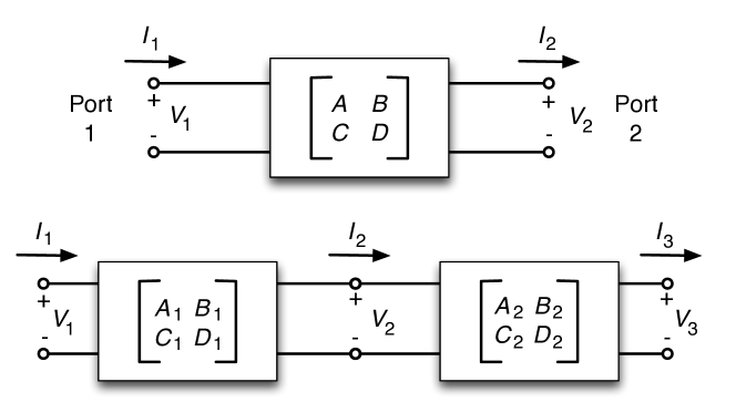
Figure 2: Top: The ABCD matrix for a 2-port network. In this diagram, voltage is denoted with $V$, and current with $I$. Bottom: Connecting two components in cascade. Diagram adapted from Pozar (2005)

3 Coherency in radio astronomy

We now turn our attention to formulating a more general RIME that is valid in a larger range of cases. In this section, we introduce the coherency matrices of Wolf (1954), along with voltage-current coherency matrices. The following section then formulates relationships between source brightness and measured coherency based upon these matrices.

3.1 Electromagnetic coherency

To begin, we introduce the coherency matrices of Wolf (1954), that fully describe the coherency statistics of an electromagnetic field. We may start by introducing $\mbox{{\emph{e}}}(\mbox{{\emph{r}}},t)$ and $\mbox{{\emph{h}}}(\mbox{{\emph{r}}},t)$ as the complex analytic representations of the electric and magnetic field vectors at a spacetime point $(\mbox{{\emph{r}}},t)$:

$$\mbox{{\emph{e}}}(\mbox{{\emph{r}}},t) =\begin{pmatrix}e_{x}(\mbox{{\emph{r}}},t)&e_{y}(\mbox{{\emph{r}}},t)&e_{z}(\mbox{{\emph{r}}},t)\end{pmatrix}^{T}$$ (23)

$$\mbox{{\emph{h}}}(\mbox{{\emph{r}}},t) =\begin{pmatrix}h_{x}(\mbox{{\emph{r}}},t)&h_{y}(\mbox{{\emph{r}}},t)&h_{z}(\mbox{{\emph{r}}},t)\end{pmatrix}^{T}$$ (24)

The coherency matrices are then defined by the formulae

$$\mbox{{\emph{E}}}_{pq}(\mbox{{\emph{r}}}_{p},\mbox{{\emph{r}}}_{q},\tau) =\begin{pmatrix}\left\langle e_{k}(\mbox{{\emph{r}}}_{p},t)e_{l}^{*}(\mbox{{\emph{r}}}_{q},t+\tau)\right\rangle\end{pmatrix}$$ (25)

$$\mbox{{\emph{H}}}_{pq}(\mbox{{\emph{r}}}_{p},\mbox{{\emph{r}}}_{q},\tau) =\begin{pmatrix}\left\langle h_{k}(\mbox{{\emph{r}}}_{p},t)h_{l}^{*}(\mbox{{\emph{r}}}_{q},t+\tau)\right\rangle\end{pmatrix}$$ (26)

$$\mbox{{\emph{M}}}_{pq}(\mbox{{\emph{r}}}_{p},\mbox{{\emph{r}}}_{q},\tau) =\begin{pmatrix}\left\langle e_{k}(\mbox{{\emph{r}}}_{p},t)h_{l}^{*}(\mbox{{\emph{r}}}_{q},t+\tau)\right\rangle\end{pmatrix}$$ (27)

$$\mbox{{\emph{N}}}_{pq}(\mbox{{\emph{r}}}_{p},\mbox{{\emph{r}}}_{q},\tau) =\begin{pmatrix}\left\langle h_{k}(\mbox{{\emph{r}}}_{p},t)e_{l}^{*}(\mbox{{\emph{r}}}_{q},t+\tau)\right\rangle\end{pmatrix}.$$ (28)

Here, $k$ and $l$ are indices representing the $x,y,z$ subscripts from Cartesian coordinates. $\mbox{{\emph{E}}}_{pq}$ and $\mbox{{\emph{H}}}_{pq}$ are called the electric and the magnetic coherency matrices, and $\mbox{{\emph{M}}}_{pq}$ and $\mbox{{\emph{N}}}_{pq}$ are called the mixed coherency matrices. The subscripts $p$ and $q$ correspond to the spacetime points $(\mbox{{\emph{r}}}_{p},t)$ and $(\mbox{{\emph{r}}}_{q},t+\tau)$, respectively. We may arrange these into a single $\mbox{6}\times\mbox{6}$ matrix $\mathbb{B}_{pq}$ that is equivalent to the time averaged outer product of the electromagnetic field column vectors at spacetime points $(\mbox{{\emph{r}}}_{p},t)$ and $(\mbox{{\emph{r}}}_{q},t+\tau)$:

$$\mathbb{B}_{pq}=\left\langle\begin{pmatrix}\mbox{{\emph{e}}}_{p}\\ \mbox{{\emph{h}}}_{p}\end{pmatrix}\otimes\begin{pmatrix}\mbox{{\emph{e}}}_{q}\\ \mbox{{\emph{h}}}_{q}\end{pmatrix}\right\rangle=\begin{pmatrix}\mbox{{\emph{E}}}_{pq}&\mbox{{\emph{M}}}_{pq}\\ \mbox{{\emph{N}}}_{pq}&\mbox{{\emph{H}}}_{pq}\end{pmatrix}$$ (29)

This matrix fully describes the coherency properties of an electromagnetic field at two points in spacetime. We will refer to this matrix as the two point coherency matrix. It is worth noting that:

• When $\mbox{{\emph{r}}}_{p}=\mbox{{\emph{r}}}_{q}$ and $\tau=0$ we retrieve what Bergman & Carozzi (2008) refer to as the ‘EM sixtor matrix’. Bergman & Carozzi (2008) show this sixtor matrix is related to what they refer to as ‘canonical electromagnetic observables’: a unique set of Stokes-like parameters that are irreducible under Lorentz transformations. These are used in the the analysis of electromagnetic field data from spacecraft.

• For monochromatic plane waves, when $\mbox{{\emph{r}}}_{p}=\mbox{{\emph{r}}}_{q}$ and $\tau=0$, and we choose a coordinate system with $z$ in the direction of propagation (i.e. along the Poynting vector), $\textbf{\emph{E}}_{pq}$ becomes what Smirnov (2011a) refers to as the brightness matrix, $\mathsf{B}$.

  From here forward, we drop the subscript $\mathbb{B}=\mathbb{B}_{00}$ and shall refer to this as the brightness coherency to highlight its relationship with $\mathsf{B}$.

3.2 Voltage and current coherency

A radio telescope converts a free space electromagnetic field into a time varying voltage, which we then measure after signal conditioning (e.g. amplification and filtering). As such, radio interferometers measure coherency statistics between time varying voltages.

One may model the analogue components of a telescope as a 6-port network, with three inputs ports and three output ports. We propose this so that there is an input-output pair of ports for each of the orthogonal components of the electromagnetic field. We can then define a set of voltages v(t) and currents $\mbox{{\emph{i}}}(t)$

$$\mbox{{\emph{v}}}(t) =\begin{pmatrix}v_{x}(t)&v_{y}(t)&v_{z}(t)\end{pmatrix}^{T}$$ (30)

$$\mbox{{\emph{i}}}(t) =\begin{pmatrix}i_{x}(t)&i_{y}(t)&i_{z}(t)\end{pmatrix}^{T}.$$ (31)

In practice, most telescopes are single or dual polarization, so only the $x$ and $y$ components are sampled. Nonetheless, it is possible to sample all three components with three orthogonal antenna elements (Bergman et al., 2005). The voltage response of an antenna is linearly related to the electromagnetic field strength (Hamaker et al., 1996), and the current is linearly related to voltage by Ohm’s law, so we may write a general linear relationship

$$\begin{pmatrix}\mbox{{\emph{v}}}(t)\\ \mbox{{\emph{i}}}(t)\end{pmatrix}=\begin{pmatrix}\mbox{{\emph{A}}}&\mbox{{\emph{B}}}\\ \mbox{{\emph{C}}}&\mathbf{\mbox{{\emph{D}}}}\end{pmatrix}\begin{pmatrix}\mbox{{\emph{e}}}(\mbox{{\emph{r}}},t)\\ \mbox{{\emph{h}}}(\mbox{{\emph{r}}},t)\end{pmatrix},$$ (32)

where A, B, C and D are block matrices forming an overall transmission matrix $\mathbb{T}^{\prime}$. We can now define a matrix of voltage-current coherency statistics that consists of the block matrices

$$\mbox{{\emph{V}}}_{pq}(\tau) =\begin{pmatrix}\left\langle v_{k}(t)v_{l}^{*}(t+\tau)\right\rangle\end{pmatrix}$$ (33)

$$\mbox{{\emph{W}}}_{pq}(\tau) =\begin{pmatrix}\left\langle i_{k}(t)i_{l}^{*}(t+\tau)\right\rangle\end{pmatrix}$$ (34)

$$\mbox{{\emph{K}}}_{pq}(\tau) =\begin{pmatrix}\left\langle v_{k}(t)i_{l}^{*}(t+\tau)\right\rangle\end{pmatrix}$$ (35)

$$\mbox{{\emph{L}}}_{pq}(\tau) =\begin{pmatrix}\left\langle i_{k}(t)v_{l}^{*}(t+\tau)\right\rangle\end{pmatrix},$$ (36)

these are analogous to (and related to) the electromagnetic coherency matrices above. In a similar manner to the two-point coherency matrix, we define $\mathbb{V}_{pq}$

$$\mathbb{V}_{pq}=\left\langle\begin{pmatrix}\mbox{{\emph{v}}}_{p}\\ \mbox{{\emph{i}}}_{p}\end{pmatrix}\otimes\begin{pmatrix}\mbox{{\emph{v}}}_{q}\\ \mbox{{\emph{i}}}_{q}\end{pmatrix}\right\rangle=\begin{pmatrix}\mbox{{\emph{V}}}_{pq}&\mathbf{\mbox{{\emph{K}}}}_{pq}\\ \mbox{{\emph{L}}}_{pq}&\mbox{{\emph{W}}}_{pq}\end{pmatrix},$$ (37)

which we will refer to as the voltage-current coherency matrix. This is analogous to the ‘visibility matrix’, $\mathsf{V}_{pq}$, of Smirnov (2011a).

4 Two point coherency relationships

Now we have introduced the two-point coherency matrix $\mathbb{B}_{pq}$ and the voltage-current coherency matrix $\mathbb{V}_{pq}$, we can formulate relationships between the two. In this section, we first formulate a general coherency relationship describing propagation from a source of electromagnetic radiation to two spacetime coordinates. We then show that this relationship underlies both the RIME and the vC-Z relationship.

4.1 A general two point coherency relationship

Suppose we have two sensors, located at points $\mbox{{\emph{r}}}_{p}$ and $\mbox{{\emph{r}}}_{q}$, which fully measure all components of the electromagnetic field. Assuming linearity, the propagation of an electromagnetic field $\mbox{{\emph{f}}}_{0}=\begin{pmatrix}\mbox{{\emph{e}}}(\mbox{{\emph{r}}}_{0},t)&\mbox{{\emph{h}}}(\mbox{{\emph{r}}}_{0},t)\end{pmatrix}^{T}$ from a point $\mbox{{\emph{r}}}_{0}$ to $\mbox{{\emph{r}}}_{p}$ and $\mbox{{\emph{r}}}_{q}$ can be encoded into a 6$\times$6 matrices, $\mathbb{T}_{p}$ and $\mathbb{T}_{q}$:

$$\mbox{{\emph{f}}}_{p} =\mathbb{T}_{p}\mbox{{\emph{f}}}_{0}$$ (38)

$$\mbox{{\emph{f}}}_{q} =\mathbb{T}_{q}\mbox{{\emph{f}}}_{0}$$ (39)

The coherency between the two signals $\mbox{{\emph{f}}}_{p}$ and $\mbox{{\emph{f}}}_{q}$ is then given by the matrix $\mathbb{B}_{pq}$:

$$\mathbb{B}_{pq} =\left\langle\mbox{{\emph{f}}}_{p}\otimes\mbox{{\emph{f}}}_{q}\right\rangle$$ (40)

$$=\left\langle(\mathbb{T}_{p}\mbox{{\emph{f}}}_{0})\otimes(\mathbf{\mathbb{T}}_{q}\mbox{{\emph{f}}}_{0})\right\rangle$$ (41)

$$=\left\langle\mathbf{\mathbb{T}}_{p}(\mbox{{\emph{f}}}_{0}\otimes\mbox{{\emph{f}}}_{0})\mathbb{T}_{q}^{H}\right\rangle$$ (42)

$$=\mathbf{\mathbb{T}}_{p}\mathbb{B}\mathbf{\mathbb{T}}_{q}^{H}$$ (43)

we can write this in terms of block matrices

$$\begin{pmatrix}\mbox{{\emph{E}}}_{pq}&\mbox{{\emph{M}}}_{pq}\\ \mbox{{\emph{N}}}_{pq}&\mbox{{\emph{H}}}_{pq}\end{pmatrix}=\begin{pmatrix}\mbox{{\emph{A}}}_{p}&\mbox{{\emph{B}}}_{p}\\ \mbox{{\emph{C}}}_{p}&\mbox{{\emph{D}}}_{p}\end{pmatrix}\begin{pmatrix}\mbox{{\emph{E}}}_{00}&\mbox{{\emph{M}}}_{00}\\ \mbox{{\emph{N}}}_{00}&\mbox{{\emph{H}}}_{00}\end{pmatrix}\begin{pmatrix}\mbox{{\emph{A}}}_{q}&\mbox{{\emph{B}}}_{q}\\ \mbox{{\emph{C}}}_{q}&\mbox{{\emph{D}}}_{q}\end{pmatrix}^{H}$$ (44)

This is the most general form that relates the coherency at two points $\mbox{{\emph{r}}}_{p}$ and $\mbox{{\emph{r}}}_{q}$, to the electromagnetic energy density at point $\mbox{{\emph{r}}}_{0}$.

In radio astronomy, antennas are used as sensors to measure the electromagnetic field. Following from Eq. 44, we may write an equation relating voltage and current coherency:

$$\mathbb{V}_{pq}=\mathbf{\mathbb{T}}{}_{p}^{{}^{\prime}}(\mathbf{\mathbb{T}}_{p}\mathbb{B}\mathbb{T}_{q}^{H})\mathbf{\mathbb{T}}{}_{q}^{{}^{\prime}H}.$$ (45)

As the $\mathbb{T}^{\prime}$ and $\mathbb{T}$ matrices are both $\mbox{6}\times\mbox{6}$ , we can are both collapse these matrices into one overall matrix. Eq. 45 then becomes

$$\mathbb{V}_{pq}=\mathbf{\mathbb{T}}{}_{p}\mathbb{B}\mathbf{\mathbb{T}}_{q}^{H},$$ (46)

which is the general form that relates the voltage-coherency matrix $\mathbb{V}_{pq}$ to the brightness coherency $\mathbb{B}.$

Equation 46 is a central result of this paper. It is a general case which relates the EM field at a given point in space-time to the voltage and current coherencies in between pairs of telescopes. In the sections that follow, we show that generalized versions of the Van-Cittert-Zernicke theorem and RIME may be formulated based upon this coherency relationship, and that the common formulations can be derived from these general results.

4.2 The Radio Interferometer Measurement Equation

By comparing Eq. 13 with Eq. 44, it is apparent that the Jones formulation of the RIME is retrieved by setting all but the top left block matrices to zero, such that we have

$$\mbox{{\emph{V}}}_{pq}=\mbox{{\emph{A}}}_{p}\mbox{{\emph{E}}}_{00}\mbox{{\emph{A}}}_{q}^{H}.$$ (47)

But under what assumptions may we ignore the other entries of Eq. 44? To answer this, we may note that monochromatic plane waves in free space have E and H are in phase and mutually perpendicular:

$$\mbox{{\emph{e}}}(\mbox{{\emph{r}}},t) =\begin{pmatrix}e_{x}(\mbox{{\emph{r}}},t)&e_{y}(\mbox{{\emph{r}}},t)\end{pmatrix}^{T}$$

$$\mbox{{\emph{h}}}(\mbox{{\emph{r}}},t) =\frac{1}{c_{0}}\begin{pmatrix}-e_{y}(\mbox{{\emph{r}}},t)&e_{x}(\mbox{{\emph{r}}},t)\end{pmatrix}^{T}$$ (48)

Where $c_{0}$ is the magnitude of the speed of light. In such a case, all coherency statistics can be derived from the $\mbox{2}\times\mbox{2}$ brightness matrix $\mathsf{B}$. Carozzi & Woan (2009) show that the field coherencies can be written

$$\mathbb{B} =\begin{pmatrix}\mbox{{\emph{E}}}_{pq}&\mbox{{\emph{M}}}_{pq}\\ \mbox{{\emph{N}}}_{pq}&\mbox{{\emph{H}}}_{pq}\end{pmatrix}=\begin{pmatrix}\mathsf{B}&\mathsf{B}\mbox{{\emph{F}}}^{T}\\ \mbox{{\emph{F}}}\mathsf{B}&\mbox{{\emph{F}}}\mathsf{B}\mbox{{\emph{F}}}^{T}\end{pmatrix}$$ (49)

where $\mathbf{F}$ is the matrix

$$\mbox{{\emph{F}}}=\frac{1}{c_{0}}\begin{pmatrix}0&1\\ -1&0\end{pmatrix}.$$ (50)

Under these conditions, the rank of $\mathbb{B}$ is 2, so the relationship in Eq. 44 is over constrained. It follows that the $\mbox{2}\times\mbox{2}$ RIME is perfectly acceptable — and indeed preferable to Eq. 44 — for describing coherency of plane waves that propagate through free space.

There are numerous situations in which we cannot assume that we have monochromatic plane waves. This includes near field sources where the wavefront is not well approximated by a plane wave; propagation through ionized gas; and situations where we choose not to treat our field as a superposition of quasi-monochromatic components. Most importantly, the assumptions that underlie the $\mbox{2}\times\mbox{2}$ RIME do not hold within the analogue components of a telescope, where the signal does not enjoy free space impedance.

4.3 A 2N-port transmission matrix based RIME

For a dual polarization telescope, a 4-port description (2-in 2-out) of our analogue system is more appropriate than the general 6-port description. Using the result 49 above and Eq. 46, we can write a relationship

$$\mbox{{\emph{V}}}_{pq}=\begin{pmatrix}\mbox{{\emph{A}}}_{p}&\mbox{{\emph{B}}}_{p}\\ \mbox{{\emph{C}}}_{p}&\mbox{{\emph{D}}}_{p}\end{pmatrix}\begin{pmatrix}\mathsf{B}&\mathsf{B}\mbox{{\emph{F}}}^{T}\\ \mbox{{\emph{F}}}\mathsf{B}&\mbox{{\emph{F}}}\mathsf{B}\mbox{{\emph{F}}}^{T}\end{pmatrix}\begin{pmatrix}\mbox{{\emph{A}}}_{q}&\mbox{{\emph{B}}}_{q}\\ \mbox{{\emph{C}}}_{q}&\mbox{{\emph{D}}}_{q}\end{pmatrix}^{H},$$ (51)

Here, all block matrices have been reduced in dimensions from $\mbox{3}\times\mbox{3}$ to $\mbox{2}\times\mbox{2}$. This version of the RIME retains the ability to model analogue components, but uses the approximations of the vC-Z to express $\mathbb{B}$ in terms of the regular $\mbox{2}\times\mbox{2}$ brightness matrix B. The transmission matrices matrices here are similar to the 2N-port transmission matrices as defined by Faria (2002).

The transmission matrices may be broken down into a chain of cascaded components. That is, for a cascade of $n$ components, we may write the overall transmission matrix as a product of matrices representing the individual components:

$$\begin{pmatrix}\mbox{{\emph{A}}}_{p}&\mbox{{\emph{B}}}_{p}\\ \mbox{{\emph{C}}}_{p}&\mbox{{\emph{D}}}_{p}\end{pmatrix}=\begin{pmatrix}\mbox{{\emph{A}}}_{np}&\mbox{{\emph{B}}}_{np}\\ \mbox{{\emph{C}}}_{np}&\mbox{{\emph{D}}}_{np}\end{pmatrix}\cdots\begin{pmatrix}\mbox{{\emph{A}}}_{1p}&\mbox{{\emph{B}}}_{1p}\\ \mbox{{\emph{C}}}_{1p}&\mbox{{\emph{D}}}_{1p}\end{pmatrix}$$ (52)

This is similar to, but more general than, Jones calculus. In the following section we will explore the difference.

4.4 Limitations of Jones calculus

Jones calculus essentially asserts two things. Firstly, it asserts that the voltage 2-vector at the output of a dual-polarization system $\mn@boldsymbol{v}_{p}=(v_{p1},v_{p2})^{T}$ is linear with respect to the EMF 2-vector $\mn@boldsymbol{e}=(e_{x},e_{y})^{T}$ at the input of the system:

$$\mn@boldsymbol{v}_{p}=\mn@boldsymbol{J}_{p}\mn@boldsymbol{e},$$ (53)

where the Jones matrix $\mn@boldsymbol{J}_{p}$ describes the voltage transmission properties of the system. The second assertion is that for a system composed of $n$ components, the effective Jones matrix is a product of the Jones matrices of the components:

$$\mn@boldsymbol{v}_{p}=\mn@boldsymbol{J}_{np}\cdots\mn@boldsymbol{J}_{1p}\mn@boldsymbol{e}.$$ (54)

With 2N-port transmission matrices, we instead describe the input of the system by the 4-vector $[\mn@boldsymbol{e},\mn@boldsymbol{h}]^{T}$, which for a monochromatic plane wave is equal to

$$\begin{pmatrix}\mn@boldsymbol{e}\\ \mn@boldsymbol{h}\end{pmatrix}=(e_{x},e_{y},-e_{y}/c_{0},e_{x}/c_{0})^{T}=\begin{pmatrix}\mn@boldsymbol{e}\\ \mn@boldsymbol{F}\mn@boldsymbol{e}\end{pmatrix},$$ (55)

and the output of the system is a 4-vector of 2 voltages and 2 currents $(\mn@boldsymbol{v}_{p},\mn@boldsymbol{i}_{p})^{T}$, which is linear with respect to the input:

$$\begin{pmatrix}\mn@boldsymbol{v}_{p}\\ \mn@boldsymbol{i}_{p}\end{pmatrix}=\begin{pmatrix}\mn@boldsymbol{A}_{p}&\mn@boldsymbol{B}_{p}\\ \mn@boldsymbol{C}_{p}&\mn@boldsymbol{D}_{p}\end{pmatrix}\begin{pmatrix}\mn@boldsymbol{e}\\ \mn@boldsymbol{F}\mn@boldsymbol{e}\end{pmatrix}.$$ (56)

Note that the output voltage is still linear with respect to the input $\mn@boldsymbol{e}$. Indeed, if one is only interested in the voltage, the above becomes

$$\mn@boldsymbol{v}_{p}=(\mn@boldsymbol{A}_{p}+\mn@boldsymbol{B}_{p}\mn@boldsymbol{F})\mn@boldsymbol{e},$$ (57)

i.e. the system has an effective Jones matrix (i.e. a voltage transmission matrix) of

$$\mn@boldsymbol{J}_{p}=\mn@boldsymbol{A}_{p}+\mn@boldsymbol{B}_{p}\mn@boldsymbol{F}.$$ (58)

However, the Jones formalism breaks down when the system is composed of multiple components. For example, with 2 components, we may naively attempt to apply Jones calculus, and describe the voltage transmission matrix of the system as a product of the components’ voltage transmission matrices:

$$\mn@boldsymbol{J}_{p}=(\mn@boldsymbol{A}_{2p}+\mn@boldsymbol{B}_{2p}\mn@boldsymbol{F})(\mn@boldsymbol{A}_{1p}+\mn@boldsymbol{B}_{1p}\mn@boldsymbol{F}),$$ (59)

i.e.

$$\mn@boldsymbol{v}_{p}=(\mn@boldsymbol{A}_{2p}\mn@boldsymbol{A}_{1p}+\mn@boldsymbol{B}_{2p}\mn@boldsymbol{F}\mn@boldsymbol{A}_{1p}+\mn@boldsymbol{A}_{2p}\mn@boldsymbol{B}_{1p}\mn@boldsymbol{F}+\mn@boldsymbol{B}_{2p}\mn@boldsymbol{F}\mn@boldsymbol{B}_{1p}\mn@boldsymbol{F})\mn@boldsymbol{e}.$$ (60)

This, however, completely neglects the current transmission properties. Applying the 2N-port transmission matrix formalism, we can see the difference:

$$\begin{pmatrix}\mn@boldsymbol{v}_{p}\\ \mn@boldsymbol{i}_{p}\end{pmatrix}=\begin{pmatrix}\mn@boldsymbol{A}_{2p}&\mn@boldsymbol{B}_{2p}\\ \mn@boldsymbol{C}_{2p}&\mn@boldsymbol{D}_{2p}\end{pmatrix}\begin{pmatrix}\mn@boldsymbol{A}_{1p}&\mn@boldsymbol{B}_{1p}\\ \mn@boldsymbol{C}_{1p}&\mn@boldsymbol{D}_{1p}\end{pmatrix}\begin{pmatrix}\mn@boldsymbol{e}\\ \mn@boldsymbol{F}\mn@boldsymbol{e}\end{pmatrix},$$ (61)

from which we can derive an expression for the voltage vector:

$$\mn@boldsymbol{v}_{p}=(\mn@boldsymbol{A}_{2p}\mn@boldsymbol{A}_{1p}+\mn@boldsymbol{B}_{2p}\mn@boldsymbol{C}_{1p}+\mn@boldsymbol{A}_{2p}\mn@boldsymbol{B}_{1p}\mn@boldsymbol{F}+\mn@boldsymbol{B}_{2p}\mn@boldsymbol{D}_{1p}\mn@boldsymbol{F})\mn@boldsymbol{e},$$ (62)

which differs from Eq. 60 in the second and fourth term of the sum, since in general

$$\mn@boldsymbol{F}\mn@boldsymbol{A}_{1p}\neq\mn@boldsymbol{C}_{1p},~{}~{}\mn@boldsymbol{F}\mn@boldsymbol{B}_{1p}\neq\mn@boldsymbol{D}_{1p}.$$ (63)

To summarize, because Jones calculus operates on voltages alone, and ignores impedance matching, we cannot use it to accurately represent the voltage response of an analogue system by a product of the voltage responses of its individual components. The difference is summarized in Eqs. 60–63; a practical example is given in Sect. 6.1. By contrast, the 2N-port transmission matrix formalism does allow us to break down the overall system response into a product of the component responses, by taking both voltages and currents into account.

Since we have now shown the $2\times 2$ form of the RIME to be insufficient, the obvious question arises, why have we been getting away with using it? Historically, practical applications of the RIME have tended to follow the formulation of Noordam (1996), rolling the electronic response of the overall system (as well as tropospheric phase, etc.) into a single ‘$G$-Jones’ term that is solved for during calibration. Under these circumstances, the $2\times 2$ formalism is perfectly adequate – it is only when we attempt to model the individual components of the analogue receiver chain that its limitations are exposed. On the other hand, Carozzi & Woan (2009) have highlighted the limitations of Jones calculus in the wide-field polarization regime.

5 Tensor formalisms of the RIME

Up until now, we have presented our $6\times 6$ RIME using matrix notation. We now briefly discuss how the work presented here is closely related to the tensor formalism presented in Smirnov (2011b).

As is discussed in Smirnov (2011b), the classical Jones formulation of the RIME is in the vector space $\mathbb{C}^{2}$. The formulation proposed by Carozzi & Woan (2009) is instead in $\mathbb{C}^{3}$. In contrast, our Eq. 46 can be considered to work in $\mathbb{C}^{6}$; that is, our EMF vector has 6 components:

$$e^{i} = \sum_{j=1}^{3}e_{j}x^{j}+\sum_{k=1}^{3}h_{j}x^{j}\equiv\sum_{j=1}^{6}e_{j}x^{j}.$$ (64)

The coherency of two voltages is once again defined via the outer product $e^{i}\bar{e}_{j}$, quite remarkably giving a (1,1)-type tensor expression identical Eq. 9 of Smirnov (2011b):

$$\mbox{\emph{V}}_{qj}^{pi}=\mbox{\emph{J}}_{\alpha}^{pi}\mbox{\emph{B}}_{\beta}^{\alpha}\bar{\mbox{\emph{J}}}_{qj}^{\beta}.$$ (65)

In the next section, we show an alternative RIME based upon a (2,0)-type tensor commonly encountered in special relativity.

5.1 A relativistic RIME

Another potential reformulation of the RIME involves the electromagnetic tensor of special relativity. The classical RIME formulation implicitly assumes that both antennas measure the EMF in the same inertial reference frame. If this is not the case (consider, e.g., space VLBI), then we must in principle account for the fact that the observed EMF is altered when moving from one reference frame to another, and in particular, that the $\mn@boldsymbol{e}$ and $\mn@boldsymbol{h}$ components intermix. In special relativity, this can be elegantly formulated in terms of the electromagnetic field tensor, which represents the 6 independent components of the EMF by a (2-0)-type tensor:

$$F^{\alpha\beta}=\left(\begin{array}[]{cccc}0&-e_{x}/c&-e_{y}/c&-e_{z}/c\\ e_{x}/c&0&-h_{z}&h_{y}\\ e_{y}/c&h_{z}&0&-h_{x}\\ e_{z}/c&-h_{y}&h_{x}&0\end{array}\right),$$ (66)

The advantage of this formulation is that the EMF tensor follows standard coordinate transform laws of special relativity. That is, for a different inertial reference frame given by the Lorentz transformation tensor $\Lambda^{\alpha}_{\alpha^{\prime}}$, the EMF tensor transforms as:

$$F^{\prime\alpha\beta}=\Lambda^{\alpha}_{\alpha^{\prime}}\Lambda^{\beta}_{\beta^{\prime}}F^{\alpha^{\prime}\beta^{\prime}}.$$ (67)

The measured 2-point coherency between $[F_{p}]$ and $[F_{q}]$ can be formally defined as the average of the outer product:

$$[V_{pq}]^{\alpha\beta\gamma\delta}=2c^{2}\langle[F_{p}]^{\alpha\beta}[F^{H}_{q}]^{\gamma\delta}\rangle,$$ (68)

where $\cdot^{H}$ represents the conjugate tensor, i.e. $[F^{H}]^{\gamma\delta}=\bar{F}^{\delta\gamma}$. A factor of 2 is introduced for the same reasons as in Smirnov (2011a), and the reason for $c^{2}$ will be apparent below. Note that the indices in the brackets should be treated as labels, while those outside the brackets are proper tensor indices.

Let us now pick a reference frame for the signal (‘frame zero’), and designate the EMF tensor in that frame by $[F_{0}]$, or $[F_{0}(\mn@boldsymbol{\bar{x}})]$ to emphasize that this is a function of the four-position $\mn@boldsymbol{\bar{x}}=(ct,\mn@boldsymbol{x})$. The $[F_{0}(\mn@boldsymbol{\bar{x}})]$ field follows Maxwell’s equations; in the case of a monochromatic plane wave propagating along direction $\mn@boldsymbol{\bar{z}}=(1,\mn@boldsymbol{z})$, this has a particularly simple solution of

$$[F_{0}(\mn@boldsymbol{\bar{x}})]=[F_{0}(\mn@boldsymbol{\bar{x}}_{0})]e^{-2\pi i\lambda^{-1}(\mn@boldsymbol{\bar{x}}-\mn@boldsymbol{\bar{x}}_{0})\cdot\mn@boldsymbol{\bar{z}}}.$$ (69)

Let us now consider two antennas located at $\mn@boldsymbol{p}$ and $\mn@boldsymbol{q}$. The 2-point coherency measured in frame zero becomes

$$[V_{pq}]^{\alpha\beta\gamma\delta} = 2c^{2}\langle[F_{0}(\mn@boldsymbol{\bar{p}})]^{\alpha\beta}[F^{H}(\mn@boldsymbol{\bar{q}})]^{\gamma\delta}\rangle$$ (70)

$$= K_{p}\left[2c^{2}\langle[F_{0}(\mn@boldsymbol{\bar{x}}_{0})]^{\alpha\beta}[F^{H}(\mn@boldsymbol{\bar{x}}_{0})]^{\gamma\delta}\rangle\right]K^{H}_{q},$$

where $K_{p}$ is the complex exponent of Eq. 69, and is the direct equivalent of the $K$-Jones term of the RIME (Smirnov, 2011a). The quantity in the square brackets is the equivalent of the brightness matrix $\mathsf{B}$, which we’ll call the brightness tensor:

$$B^{\alpha\beta\gamma\delta}=[B_{0}]^{\alpha\beta\gamma\delta}=2c^{2}\langle[F_{0}(\mn@boldsymbol{\bar{x}}_{0})]^{\alpha\beta}[F_{0}^{H}(\mn@boldsymbol{\bar{x}}_{0})]^{\gamma\delta}\rangle.$$ (71)

Each element of the brightness tensor gives the coherency between two components of the EMF observed in the chosen reference frame (‘frame zero’). Nominally, the brightness tensor has $4^{4}=256$ components, but only 36 are unique and non-zero (given the 6 components of the EMF). Carozzi & Bergman (2006) show that the brightness tensor may be decomposed into a set of antisymmetric second rank tensors (‘sesquilinear-quadratic tensor concomitants’) that are irreducible under Lorentz transformations. The physical interpretation of the 36 unique quantities within the brightness matrix is discussed in Bergman & Carozzi (2008), with regards to the aforementioned irreducible tensorial set.

While the brightness tensor has redundancy not present in the tensorial set of Carozzi & Bergman (2006), we shall continue to use it as a basis to our relativistic RIME for clarity of analogy to the brightness coherency matrix of Eq. 46, and as it leads to a relativistic RIME for which we can define transformation tensors analogous to Jones matrices. The redundancy can be described by a number of symmetry properties of the brightness tensor: it is (a) Hermitian with respect to swapping the first and second pair of indices:

$$B^{\alpha\beta\gamma\delta}=\bar{B}^{\gamma\delta\alpha\beta},$$ (72)

(b) antisymmetric within each index pair (since the EMF tensor itself is antisymmetric, i.e. $F^{\alpha\beta}=-F^{\beta\alpha}$):

$$B^{\alpha\beta\gamma\delta}=-B^{\beta\alpha\gamma\delta}=-B^{\alpha\beta\delta\gamma}$$ (73)

To see the direct analogy to the brightness matrix, consider again the case of the monochromatic plane wave propagating along $\mn@boldsymbol{z}$ (Eq. 48). The EMF tensor then takes a particularly simple form:

$$F^{\alpha\beta}=\frac{1}{c}\left(\begin{array}[]{cccc}0&-e_{x}&-e_{y}&0\\ e_{x}&0&0&e_{x}\\ e_{y}&0&0&e_{y}\\ 0&-e_{x}&-e_{y}&0\end{array}\right),$$ (74)

and the brightness tensor has only $8^{2}=64$ non-zero components, with the additional ‘0-3’ symmetry property:

$$B^{0\beta\gamma\delta}=B^{3\beta\gamma\delta} B^{\alpha 0\gamma\delta}=B^{\alpha 3\gamma\delta}$$

$$B^{\alpha\beta 0\delta}=B^{\alpha\beta 3\delta} B^{\alpha\beta\gamma 0}=B^{\alpha\beta\gamma 3}$$ (75)

Four unique components can be defined in terms of the Stokes parameters:

$$B^{0110}=I+Q B^{0220}=I-Q$$

$$B^{0120}=U+iV B^{0210}=U-iV$$ (76)

and conversely,

$$I=\frac{B^{0110}+B^{0220}}{2} Q=\frac{B^{0110}-B^{0220}}{2},$$

$$U=\frac{B^{0120}+B^{0210}}{2} V=\frac{B^{0120}-B^{0210}}{2i}.$$ (77)

The other non-zero components of the brightness tensor can be derived using the Hermitian, antisymmetry and 0-3 symmetry properties. Finally, for an unpolarized plane wave, only 32 components of the brightness tensor are non-zero and equal to $\pm I$. As these will be useful in further calculations, they are summarized in Table 1.

	01	02	10	13	20	23	31	32
01	$-I$		$I$	$I$			$-I$
02		$-I$			$I$	$I$		$-I$
10	$I$		$-I$	$-I$			$I$
13	$I$		$-I$	$-I$			$I$
20		$I$			$-I$	$-I$		$I$
23		$I$			$-I$	$-I$		$I$
31	$-I$		$I$	$I$			$-I$
32		$-I$			$I$	$I$		$-I$

Table 1: The non-zero components of the brightness tensor $B^{\alpha\beta\gamma\delta}$ for an unpolarized plane wave. Rows correspond to $\alpha\beta$, columns to $\gamma\delta$.

So far this has been nothing more than a recasting of the RIME using EMF tensors. Consider, however, the case where antennas $p$ and $q$ measure the signal in different inertial reference frames. The EMF tensor observed by antenna $p$ becomes

$$[F_{p}]^{\alpha\beta}=[\Lambda_{p}]^{\alpha}_{\alpha^{\prime}}[\Lambda_{p}]^{\beta}_{\beta^{\prime}}[F_{0}]^{\alpha^{\prime}\beta^{\prime}},$$ (78)

where $[\Lambda_{p}]^{\alpha}_{\mu}$ is the Lorentz tensor corresponding to the transform between the signal frame and the antenna frame. Since the same Lorentz tensor always appears twice in these equations (due to $F$ being a (2,0)-type tensor), let us designate

$$[\Lambda_{p}]^{\alpha\beta}_{\alpha^{\prime}\beta^{\prime}}=[\Lambda_{p}]^{\alpha}_{\alpha^{\prime}}[\Lambda_{p}]^{\beta}_{\beta^{\prime}}$$ (79)

for compactness. The measured coherency now becomes

$$[V_{pq}]^{\alpha\beta\gamma\delta}=K_{p}{[\Lambda_{p}]}^{\alpha\beta}_{\alpha^{\prime}\beta^{\prime}}[B_{0}]^{\alpha^{\prime}\beta^{\prime}\gamma^{\prime}\delta^{\prime}}[\Lambda_{q}]^{\gamma\delta}_{\gamma^{\prime}\delta^{\prime}}K^{H}_{q}.$$ (80)

The equivalent of Jones matrices would be (2,2)-type ‘Jones tensors’ $J^{\alpha\beta}_{\alpha^{\prime}\beta^{\prime}}$, so a more general formulation of the above would be

$$[V_{pq}]^{\alpha\beta\gamma\delta}={[J_{p}]}^{\alpha\beta}_{\alpha^{\prime}\beta^{\prime}}[B_{0}]^{\alpha^{\prime}\beta^{\prime}\gamma^{\prime}\delta^{\prime}}[J^{H}_{q}]^{\gamma\delta}_{\gamma^{\prime}\delta^{\prime}},$$ (81)

where tensor conjugation $\cdot^{H}$ is defined as:

$$[J^{H}]^{\alpha\beta}_{\alpha^{\prime}\beta^{\prime}}=\bar{J}^{\beta\alpha}_{\beta^{\prime}\alpha^{\prime}}.$$ (82)

Note that both the $K$ and $\Lambda$ terms of Eq. 80 can be considered as special examples of Jones tensors. The $K$ term can be explicitly written as a (2,2)-type tensor via two Kronecker deltas:

$$[K_{p}]^{\alpha\beta}_{\alpha^{\prime}\beta^{\prime}}=K_{p}\delta^{\alpha}_{\alpha^{\prime}}\delta^{\beta}_{\beta^{\prime}},$$ (83)

while the $\Lambda$ term is a (2,2)-type tensor by definition (Eq. 79), noting that

$$[\Lambda^{H}_{p}]^{\alpha\beta}_{\alpha^{\prime}\beta^{\prime}}=[\Lambda_{p}]^{\alpha\beta}_{\alpha^{\prime}\beta^{\prime}},$$ (84)

since the components of any Lorentz transformation tensor $\Lambda^{\alpha}_{\alpha^{\prime}}$ are real.

Finally, let us note the equivalent of the ‘chain rule’ for Jones tensors. If the signal chain is represented by a sequence of Jones tensors $[J_{p,n}],...,[J_{p,1}]$ (including $K$ terms, $\Lambda$ terms, and all instrumental and propagation effects), then the overall response is given by

$$[J_{p}]^{\alpha\beta}_{\alpha^{\prime}\beta^{\prime}}=[J_{p,n}]^{\alpha\beta}_{\alpha_{n}\beta_{n}}[J_{p,n-1}]^{\alpha^{n}\beta^{n}}_{\alpha_{n-1}\beta_{n-1}}\cdots[J_{p,1}]^{\alpha^{2}\beta^{2}}_{\alpha^{\prime}\beta^{\prime}}.$$ (85)

Equations 80, 81 and 85 above constitute a relativistic reformulation of the RIME (RRIME). The RRIME allows us to incorporate relativistic effects into our measurement equation. That is, we can treat relativistic motion as an ‘instrumental’ effect. Some interesting observational consequences, and the relation of the RRIME to work from other fields are treated in the discussion below.

6 Discussion

The formulations presented here highlight the relationship between the seemingly disparate fields of microwave networking and special relativity to measurements in radio astronomy. This is a remarkable illustration of how these fields are intrinsically related by underlying fundamental physics.

Indeed, it has long been known that Jones and Mueller transformation matrices are related to Lorentz transformations by the Lorentz group. Wiener was aware as early as 1928 that the the 2$\times$2 coherency matrix could be written in terms of the Pauli spin matrices (Wiener, 1928, 1930). More recently, Baylis et al. (1993) presents a more general geometric algebra formalism that unifies Jones and Mueller matrices with Stokes parameters and the Poincaré sphere. Han et al. (1997b) show that the Jones formalism is a representation of the six-parameter Lorentz group; further to this Han et al. (1997a) show that the Stokes parameters form a Minkowskian four-vector, similar to the energy-momentum four-vector in special relativity.

In contrast, the RRIME presented here is novel as it fully describes interferometric measurement between two points, instead of simply describing polarization states and defining a transformation algebra. Similarly, the 2N-port RIME specifically shows how microwave networking methods can be incorporated into a ME.

What do we gain from using these more general measurement equations in lieu of the simpler 2$\times$2 RIME? For most applications, it will suffice to simply be aware of the standard RIME’s limitations, and to work in a piecemeal fashion. For example, one can quite happily use Jones matrices to describe free space propagation, and microwave network methods to describe discrete analogue components. An overall ‘system Jones’ matrix may be derived to describe instrumental effects, but this matrix should never be decomposed into a Jones chain.

Similarly, special relativity describes relativistic effects through Lorentz transformations acting upon the EMF tensor. We can treat relativistic motion as an instrumental effect by using the RRIME, or we can apply special relativistic corrections separately, as required. The effect of relativistic boosts on the Stokes parameters are considered in Cocke & Holm (1972).

In the subsections that follow, we present some potential use cases that highlight the usefulness of the 2N-port and relativistic RIME formulations.

6.1 Modelling real analogue components

The 2N-port RIME may have practicality in absolute flux calibration of radio telescopes. Generally, interferometer data is calibrated by assuming that the sky brightness is known, or at least approximately known. If we wish to do absolute calibration of a telescope without making assumptions about the sky, we must instead make sure that we accurately model the analogue components of our telescope. A particularly ubiquitous method of device characterization within microwave engineering is the use of scattering parameters; we briefly introduce these below before incorporating them into the 2N-port RIME.

6.1.1 Scattering parameters

Voltage, current and impedance are somewhat abstract concepts at microwave frequencies, so engineers often use scattering parameters to quantify a device’s characteristics. Scattering parameters relate the incident and reflected voltage waves on the ports of a microwave network. The scattering matrix, S, is given by

$$\begin{pmatrix}v_{1}^{-}\\ v_{2}^{-}\\ \vdots\\ v_{n}^{-}\end{pmatrix}=\begin{pmatrix}S_{11}&S_{12}&\cdots&S_{1n}\\ S_{21}&&&\vdots\\ \vdots&&\ddots&\vdots\\ S_{n1}&\cdots&\cdots&S_{nn}\end{pmatrix}\begin{pmatrix}v_{1}^{+}\\ v_{2}^{+}\\ \vdots\\ v_{n}^{+}\end{pmatrix},$$ (86)

where $v_{n}^{+}$ is the amplitude of the voltage wave incident on port $n$, and $v_{n}^{-}$ is the amplitude of the voltage wave reflected from port $n$.

For a dual polarization system (we will label the polarization x and y) with negligible crosstalk, we can model the analogue chain for each polarization as a discrete 2-port network. Assuming that the analogue chains have the same number of components (but not that the components are identical), the transmission matrix for each pair of components is

$$\mbox{{\emph{T}}}=\begin{pmatrix}\tilde{A}_{x}&0&\tilde{B}_{x}&0\\ 0&\tilde{A}_{y}&0&\tilde{B}_{y}\\ \tilde{C}_{x}&0&\tilde{D}_{x}&0\\ 0&\tilde{C}_{y}&0&\tilde{D}_{y}\end{pmatrix},$$ (87)

where the elements are from the ABCD matrices of the x and y polarizations, and are given by the relations

$$\tilde{A} =\frac{1+S_{12}S_{21}+S_{22}-S_{11}(1+S_{22})}{2S_{12}}$$ (88)

$$\tilde{B} =-Z_{0}\frac{1+S_{11}-S_{12}S_{21}+S_{22}+S_{11}S_{22}}{2S_{12}}$$ (89)

$$\tilde{C} =\frac{1}{Z_{0}}\frac{-1+S_{11}+S_{12}S_{21}+S_{22}-S_{11}S_{22}}{2S_{12}}$$ (90)

$$\tilde{D} =\frac{1+S_{11}+S_{12}S_{21}-S_{22}-S_{11}S_{22}}{2S_{12}}$$ (91)

Here, $Z_{0}$ is the characteristic impedance of the analogue chain, which in most telescopes is set to 50 or 75 ohms. We have added tildes to the ABCD parameters, as we are using the inverse definition to that in Pozar (2005).

If the system has significant crosstalk between polarizations, the analogue chain is more accurately modelled as a 4-port network. In this case the relationships are not so simple, and the off-diagonal entries of the block matrices of T will no longer be zero.

6.1.2 Scattering matrix example

We now present a simple illustration of the differences between assigning a component a scalar value (as is done in the Jones formalism), and by modelling it as a 2-port network. Consider a component with a scattering matrix

$$\mbox{{\emph{S}}}=\begin{pmatrix}0.1\angle 0^{\circ}&0.9\angle 0^{\circ}\\ 0.9\angle 0^{\circ}&0.1\angle 0^{\circ}\end{pmatrix}$$ (92)

for a given quasi-monochromatic frequency. Here, values are presented in angle notation to emphasize that they are complex valued. In decibels, the $S_{11}$ and $S_{22}$ parameters have a magnitude of -10 dB, and the $S_{12}$ and $S_{21}$ parameters have a magnitude of about $-0.5$ dB. Now suppose we have three identical copies of this component, and we connect them together in cascade. If one only considered the forward gain ($S_{21}$), one would arrive at an overall $S_{\rm{21tot}}$ of

$$S_{\rm{21tot}}=S_{21}S_{21}S_{21}=0.729$$ (93)

In contrast, using the standard microwave engineering methods, we can form a transmission matrix (using equations 88-91 above), and then convert this back into an overall matrix, $\mbox{{\emph{S}}}_{\rm{tot}}$. By doing this, one finds

$$\mbox{{\emph{S}}}_{\rm{cas}}=\begin{pmatrix}0.25\angle 0^{\circ}&0.75\angle 0^{\circ}\\ 0.75\angle 0^{\circ}&0.25\angle 0^{\circ}\end{pmatrix}.$$ (94)

The difference becomes more marked as $S_{11}$ and $S_{22}$ increase; as $S_{11}$ and $S_{22}$ approach zero, the two methods converge.

When designing a component, $S_{11}$ and $S_{22}$ are generally optimised to be as small as possible over the operational bandwidth. Nevertheless, their affect on the overall system is often non-negligible.

6.1.3 Absolute calibration experiments

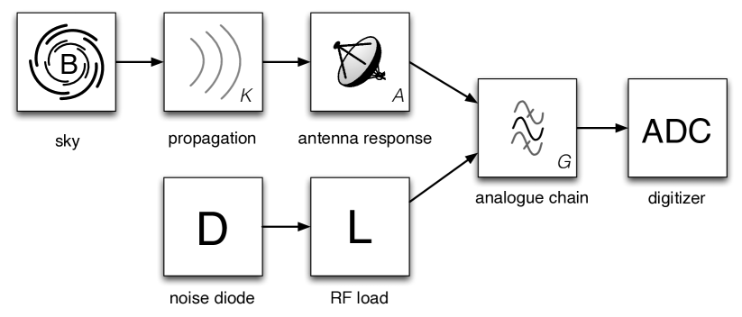
Figure 3: Block diagram of a three-state switching experiment. In addition to the antenna path, an RF load can in series with a noise diode can be selected. The noise diode can be turned on and off, giving three possible states: antenna, load, and diode + load. These three states are used for instrumental calibration.

Now we have shown how scattering parameters can be used within the 2N-port RIME, we turn our attention to the challenges of absolute calibration of radio telescopes. Measurement of the absolute flux of radio sources is fiendishly hard; as such, almost all calibrated flux data presented in radio astronomy literature are pinned to the flux scale presented in Baars et al. (1977), either directly or indirectly (Kellermann, 2009). Recent experiments, such as the Experiment to Detect the Global EoR Step (EDGES, Bowman & Rogers 2010), and the Large-Aperture Experiment to detect the Dark Ages (LEDA, Greenhill & Bernardi 2012), are seeking to make precision measurement of the sky temperature (i.e. total power of the sky brightness) as a function of frequency. The motivation for this is to detect predicted faint (mK) spectral features imprinted on the sky temperature due to coupling between the microwave background and neutral Hydrogen in the early universe. For such instruments — and other instruments with wide field-of-views — this flux ‘bootstrapping’ method is not sufficient.

For experiments such as EDGES a thorough understanding of the analogue systems is vital to control the systematics that confound calibration. The calibration strategy used for EDGES is detailed in Rogers & Bowman (2012), and consists of a novel three-state switching and rigorous scattering parameter measurements with a Vector Network Analyzer (VNA) to remove the bandpass and characterize the antenna.

Our 2N-port RIME allow for scattering parameters to be directly incorporated into a measurement equation that relates sky brightness to measured voltages at the digitizer. This could be used either to (a) infer the scattering parameters of a device given a known sky brightness, or (b) infer the sky brightness from precisely measured scattering parameters. The EDGES approach is the latter, but via an ad-hoc method without formal use of a ME.

6.1.4 A three-state switching measurement equation

The three-state switching as described in Rogers & Bowman (2012) involves switching between the antenna and a reference load and noise diode, and measuring the resultant power spectra ($P_{A}$, $P_{L}$, and $P_{D}$, respectively). This is shown as a block diagram in Figure 3. The power as measured in each state is then given by:

$$P_{A} = Gk_{B}\Delta\nu(T_{A}+T_{\rm{rx}})$$ (95)

$$P_{L} = Gk_{B}\Delta\nu(T_{L}+T_{\rm{rx}})$$ (96)

$$P_{D} = Gk_{B}\Delta\nu(T_{D}+T_{L}+T_{\rm{rx}})$$ (97)

where $k_{B}$ is the Boltzmann constant, $T_{D}$ and $T_{L}$ are the diode and reference load noise temperatures, $T_{\rm{rx}}$ is the receiver’s noise temperature, $G$ is the system gain, and $\Delta\nu$ is bandwidth. One can recover the antenna temperature $T_{A}$ by

$$T_{A}=T_{D}\frac{P_{A}-P_{L}}{P_{D}-P_{L}}+T_{L},$$ (98)

where the diode and load temperatures, $T_{D}$ and $T_{L}$, are known. Antenna temperature is then related to the sky temperature by

$$T_{\rm{sky}}=T_{A}(1-|\Gamma|^{2}),$$ (99)

where the reflection coefficient $\Gamma\equiv S_{11}$. Failure to account for reflections (i.e. impedance mismatch) results in an unsatisfactory calibration, due to standing waves within the coaxial cable that manifest as a sinusoidal ripple on $T_{A}=T_{A}(\nu)$. This effect is a prime example why one must not use Jones matrices to describe analogue components separately; an example showing a standing wave present on three-state switch calibrated spectrum from a prototype LEDA antenna is shown in Figure 4.

We may instead write the equations above in terms of 2N-port transmission matrices, and form MEs for the three states:

$$\mathbf{V}_{A} = \mathbf{G}(\mathbf{T}_{A}\mathbb{B}_{\rm{sky}}\mathbf{T}_{A}^{H}+\mathbb{B}_{\rm{rx}})\mathbf{G}^{H}$$ (100)

$$\mathbf{V}_{L} = \mathbf{G}(\mathbb{B}_{L}+\mathbb{B}_{\rm{rx}})\mathbf{G}^{H}$$ (101)

$$\mathbf{V}_{D} = \mathbf{G}(\mathbf{T}_{L}\mathbb{B}_{D}\mathbf{T}_{L}^{H}+\mathbb{B}_{L}+\mathbb{B}_{\rm{rx}})\mathbf{G}^{H}.$$ (102)

Here, we have replaced the scalar powers $P_{A,L,D}$ with corresponding voltage-coherency matrices $\mathbf{V}_{A,L,D}$, temperatures $T_{A,L,\rm{sky},\rm{rx}}$ are replaced with brightness matrices $\mathbb{B}_{A,L,\rm{sky},\rm{rx}}$, and $Gk_{B}$ is instead represented by a system gain matrix $\mathbf{G}$. We have added a transmission matrix for the antenna $\mathbf{T}_{A}$, and a transmission matrix $\mathbf{T}_{L}$ for the load in series with the noise diode. Note that the relation of Eq. 99 is now encoded into the ME by the matrix $\mathbf{T}_{A}$, and that we have dropped antenna number subscripts as p=q for autocorrelation measurements.

It is immediately apparent that the cancellations that occur in the ratio of Eq. 98 will not in general occur for the equivalent ratio $\mathbf{R}=(\mathbf{V}_{A}-\mathbf{V}_{L})(\mathbf{V}_{D}-\mathbf{V}_{L})^{-1}$. We can however retrieve the result of Eq. 98 by treating the two polarizations separately, setting $\mathbf{G}=G\mathbf{I}$ and $\mathbf{T}_{L}=\mathbf{I}$, with $\mathbf{T}_{A}=T_{A}(1-|\Gamma|^{2})\mathbf{I}$.

Our equations Eq. 100-102 allow for both polarizations to be treated together, which will be important if cross-polarization terms are non-negligible. Also, we may expand Eq. 100 to include ionospheric effects. This ability to combine all effects into a single ME may simplify data analysis and improve calibration accuracy for such experiments.

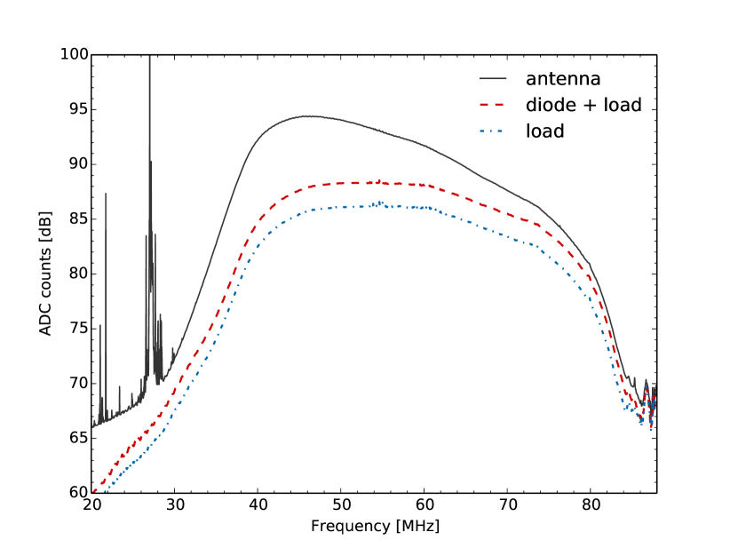
(a) .

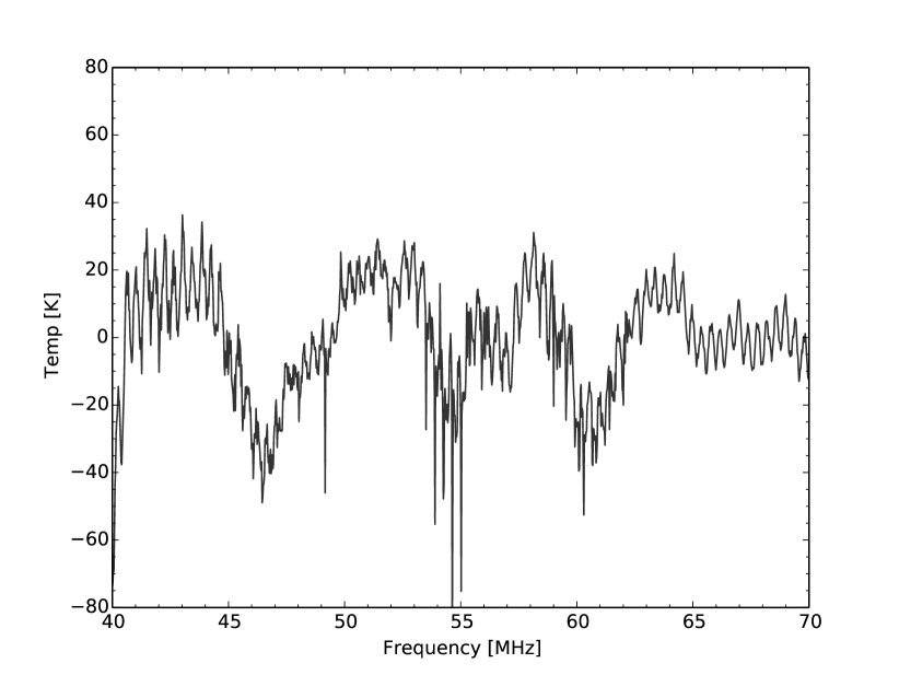
(b)

Figure 4: (a) Data from a LEDA three-state switched antenna during a testing campaign in December, 2013. These correspond to the $P_{A}$, $P_{L}$, and $P_{D}$ of Eqns. 95-97. (b) Residuals after applying Eq. 98, to the data shown in Fig. 4a and removing an antenna model power-law fit. The fast varying sinusoid can be attributed standing waves along the $\sim$300 m of coaxial cable connecting the antenna to the back-end electronics; the sharp negative spikes are due to radio interference.

6.2 RRIME and Lorentz boosts

To illustrate how the RRIME can be used to describe relativistic effects, let us first consider the ‘simple’ case of a relativistically moving source. Suppose we have an unpolarized point source (Table 1), with antennas $p$ and $q$ located in the $xy$ plane perpendicular to the direction of propagation $z$ (so the $K$ component becomes unity), both moving parallel to the $x$ axis with velocity $v$. The Lorentz transformation tensor from the signal frame to the antenna frame is then

$$[\Lambda_{p}]^{\alpha}_{\alpha^{\prime}}=\left(\begin{array}[]{cccc}\gamma&-\beta\gamma&0&0\\ -\beta\gamma&\gamma&0&0\\ 0&0&1&0\\ 0&0&0&1\end{array}\right),$$ (103)

where

$$\beta=\frac{v}{c},~{}~{}\gamma=\frac{1}{\sqrt{1-\beta^{2}}}.$$ (104)

The Lorentz factor $\gamma$ is unity 1 at $v=0$, and goes to infinity with $v\rightarrow c$. This case can be analyzed without invoking coherencies. Consider the EMF, which in the signal frame is a plane wave (Eq. 74). In the antenna frame it becomes

$$[F_{p}]^{\alpha\beta}=\frac{1}{c}\left(\begin{array}[]{cccc}0&-e_{x}&-\gamma e_{y}&-\beta\gamma e_{x}\\ e_{x}&0&\beta\gamma e_{y}&\gamma e_{x}\\ \gamma e_{y}&-\beta\gamma e_{y}&0&e_{y}\\ \beta\gamma e_{x}&-\gamma e_{x}&-e_{y}&0\end{array}\right).$$ (105)

Noting that

$$\left(\begin{array}[]{ccc}\gamma^{-1}&0&\beta\\ 0&1&0\\ -\beta&0&\gamma^{-1}\end{array}\right)\left(\begin{array}[]{c}e_{x}\\ \gamma e_{y}\\ \beta\gamma e_{x}\end{array}\right)=\gamma\left(\begin{array}[]{c}e_{x}\\ e_{y}\\ 0\end{array}\right),$$ (106)

and

$$\left(\begin{array}[]{ccc}\gamma^{-1}&0&\beta\\ 0&1&0\\ -\beta&0&\gamma^{-1}\end{array}\right)\left(\begin{array}[]{c}-e_{y}\\ \gamma e_{x}\\ -\beta\gamma e_{y}\end{array}\right)=\gamma\left(\begin{array}[]{c}-e_{y}\\ e_{x}\\ 0\end{array}\right),$$ (107)

and $\gamma^{-2}+\beta^{2}=1,$ we can see that the EMF in the antenna frame is equivalent to a boost of the original EMF by $\gamma$ (also called Doppler boost), coupled to a rotation through $\phi=-\cos^{-1}\beta$ in the $xz$ plane (i.e. the direction of propagation appears to change, also called relativistic aberration). Both effects are well-understood in the guise of relativistic beaming, and explain why, for example, some AGNs exhibit asymmetric jets (see e.g. Sparks et al., 1992).

From an RRIME point of view, a more interesting case arises when one antenna is moving with respect to the other (as is the case in space VLBI). Let’s consider antenna $p$ to be at rest with respect to the signal frame (so the $[\Lambda_{p}]^{\alpha\beta}_{\alpha^{\prime}\beta^{\prime}}$ component becomes the equivalent of unity – the product of two Kronecker deltas – and thus may be dropped), and antenna to be $q$ moving parallel to the $x$ axis with velocity $v$. The $[J_{q}]^{\gamma\delta}_{\gamma^{\prime}\delta^{\prime}}$ tensor in Eq.  81 is then a product of two Lorentz tensors of the form of Eq. 103. In the absence of other effects, the measured coherency becomes

$$[V_{pq}]^{\alpha\beta\gamma\delta}=B^{\alpha\beta\gamma^{\prime}\delta^{\prime}}[\Lambda_{q}]^{\gamma}_{\gamma^{\prime}}[\Lambda_{q}]^{\delta}_{\delta^{\prime}},$$ (108)

or writing it out as an explicit sum for two particular elements of interest (and dropping the $pq$ indices):

$$V^{0110} = \sum_{\gamma\delta}B^{01\gamma\delta}[\Lambda_{q}]^{0}_{\gamma}[\Lambda_{q}]^{1}_{\delta}$$ (109)

$$V^{0220} = \sum_{\gamma\delta}B^{02\gamma\delta}[\Lambda_{q}]^{0}_{\gamma}[\Lambda_{q}]^{2}_{\delta}.$$ (110)

Each sum above nominally contains 16 terms, but if we assume an unpolarized point source, then from Table 1 (looking up rows ‘01’ and ‘02’) we note that only four components of $B$ in each sum are non-zero. Combining this with Eq. 103, we get:

$$V^{0110}=I(\gamma^{2}-\beta^{2}\gamma^{2})=I,$$ (111)

and

$$V^{0220}=I\gamma.$$ (112)

Doing the same sums for $V^{0120}$ and $V^{0210}$, we arrive at zero. This implies that our instrument will measure the Stokes parameters as

$$I_{\mathrm{meas}} = \frac{V^{0110}+V^{0220}}{2}=I\frac{1+\gamma}{2}$$ (113)

$$Q_{\mathrm{meas}} = \frac{V^{0110}-V^{0220}}{2}=I\frac{1-\gamma}{2}$$ (114)

$$U_{\mathrm{meas}} = 0$$ (115)

$$V_{\mathrm{meas}} = 0.$$ (116)

Since $\gamma>1$, we measure boost in the total power $I$, and negative apparent $Q$ (that is, linear polarization perpendicular to the direction of motion). The physical meaning of this instrumental $Q$ can be understood in terms of the polarization aberration discussed by Carozzi & Woan (2009): because the arriving plane wave is aberrated in the frame of antenna $q$ (i.e. no longer appears to propagate along the $z$ axis, but along a slightly different direction), it is measured as polarized by dipoles that are parallel to $xy$.

Note that this formulation does not incorporate the Doppler shift observed by a moving antenna (we quietly assume that the correlator takes care of correcting for this when channelizing), or the problems of clock distribution to a relativistically moving observing platform. This will have to be addressed in a future work.

In principle, the effects of Doppler boost and relativistic aberration can be described without invoking the full RRIME – traditional Jones calculus still suffices. However the RRIME provides a unifying framework that allows these effects to be incorporated into a single compact interferometric measurement equation. This is similar to how the original RIME formulation of Hamaker et al. (1996) incorporated polarimetric effects that were already described previously (Sault et al., 1991) in a compact closed form.

An even more interesting use case arises when the incident EMF can no longer be described by a plane wave. The EMF tensor of Eq. 66 then no longer reduces to Eq. 74, or in other words, the $\mn@boldsymbol{e}$ and $\mn@boldsymbol{h}$ components of the EM are no longer mutually redundant. Under Lorentz transformations, the $\mn@boldsymbol{e}$ and $\mn@boldsymbol{h}$ components then become intermixed – an antenna measuring $\mn@boldsymbol{e}$ in the rest frame will also measure some contribution from $\mn@boldsymbol{h}$ in a moving frame. It is clear that in this case, Jones calculus (which only operates on $\mn@boldsymbol{e}$) can no longer apply, and a full RRIME must be invoked. Practical applications of this will have to wait for near-field space VLBI.

Conceptually, the latter example is very similar to the transmission matrix formalism. In a system where the voltage and current components intermix, the voltage-only Jones formalism no longer applies, and a formalism incorporating both components must be invoked.

7 Conclusions

The radio interferometer Measurement Equation provides a powerful framework for describing a signal’s journey from an astrophysical source to the receiver of a radio telescope. Nevertheless, the Jones calculus it employs is in general not sufficient to describe the components within the analogue chain of a radio telescope. Within the telescope, methods from microwave network theory, such as transmission matrices and scattering parameters, are more appropriate.

Similarly, the Jones formalism is not able to describe relativistic effects. We have presented two reformulations that account for mixed and magnetic field coherency in a way that is not possible with the Jones formalism. These reformulations extend the applicability of the RIME to allow it to correctly model analogue components, and to describe relativistic effects within the RIME.

References

- Baars et al. (1977) Baars J. W. M., Genzel R., Pauliny-Toth I. I. K., Witzel A., 1977, A&A, 61, 99
- Baylis et al. (1993) Baylis W. E., Bonenfant J., Derbyshire J., 1993, Am. J. Phys., 61, 534
- Bergman et al. (2005) Bergman J. E. S. et al., 2005, in DGLR intl. symp. ”To Moon and Beyond”
- Bergman & Carozzi (2008) Bergman J. E. S., Carozzi T. D., 2008, arXiv, astro-ph/0804.2092
- Bowman & Rogers (2010) Bowman J., Rogers A., 2010, Nature, 468, 796
- Carozzi & Bergman (2006) Carozzi T. D., Bergman J. E. S., 2006, J. Mat. Phys., 47, 2903
- Carozzi & Woan (2009) Carozzi T. D., Woan G., 2009, MNRAS, 395, 1558
- Cocke & Holm (1972) Cocke W. J., Holm D. A., 1972, Nature Physical Science, 240, 161
- Faria (2002) Faria J. A. B., 2002, Microwave and Optical Technology Letters, 33, 151
- Greenhill & Bernardi (2012) Greenhill L. J., Bernardi G., 2012, in NARIT Conf. Ser., Komonjinda S. S., Kovalev Y. Y., Ruffolo D., eds., Vol. 1
- Hamaker (2000) Hamaker J. P., 2000, A&A Supp., 143, 515
- Hamaker (2006) Hamaker J. P., 2006, A&A, 456, 395
- Hamaker & Bregman (1996) Hamaker J. P., Bregman J. D., 1996, A&A Supp., 117, 161
- Hamaker et al. (1996) Hamaker J. P., Bregman J. D., Sault R. J., 1996, A&A Supp., 117, 137
- Han et al. (1997a) Han D., Kim Y., Noz M., 1997a, Phys. Rev. E, 56, 6065
- Han et al. (1997b) Han D., Kim Y. S., Noz M. E., 1997b, J. Opt. Soc. Am., 14, 2290
- Jones (1941) Jones R. C., 1941, J. Opt. Soc. Am., 31, 1
- Kellermann (2009) Kellermann K. I., 2009, A&A, 500, 143
- Mandel & Wolf (1995) Mandel L., Wolf E., 1995, Optical Coherence and Quantum Optics, 1st edn. Cambridge University Press
- Mueller (1948) Mueller H., 1948, J. Opt. Soc. Am., 38, 661
- Noordam (1996) Noordam J. E., 1996, AIPS++ Note 185. Tech. rep., AIPS++
- Pozar (2005) Pozar D. M., 2005, Microwave Engineering, 3rd edn. John Wiley and Sons Inc.
- Rogers & Bowman (2012) Rogers A. E. E., Bowman J. D., 2012, Radio Science, 47, RS0K06
- Sault et al. (1991) Sault R., Killeen N., Kesteven M., 1991, AT polarisation calibration. Tech. Rep. 39.3/015, ATNF
- Sault et al. (1996) Sault R. J., Hamaker J. P., Bregman J. D., 1996, A&A Supp., 117, 149
- Smirnov (2011a) Smirnov O. M., 2011a, A&A, 527, A106
- Smirnov (2011b) Smirnov O. M., 2011b, A&A, 531, A159
- Sparks et al. (1992) Sparks W. B., Fraix-Burnet D., Macchetto F., Owen F. N., 1992, Nature, 355, 804
- Taylor et al. (1999) Taylor G. B., Carilli C. L., Perley R. A., eds., 1999, Synthesis Imaging in Radio Astronomy II, Vol. 180. ASP
- Thompson et al. (2004) Thompson A. R., Moran J. M., Jr. G. W. S., 2004, Interferometry and Synthesis in Radio Astronomy, 2nd edn. WILEY-VCH Verlag
- Wiener (1928) Wiener N., 1928, J. Mat. Phys., 7, 109
- Wiener (1930) Wiener N., 1930, Acta Mathematica, 55, 117
- Wolf (1954) Wolf E., 1954, Nuovo Cimento, 12
- Zernicke (1938) Zernicke F., 1938, Physica, 5