Replica Symmetric Bound for
Restricted Isometry Constant

Ayaka Sakata The Institute of Statistical Mathematics
Tachikawa, Japan
Theoretical Biology Laboratory
RIKEN, Wako, Japan
Email: ayaka@ism.ac.jp
   Yoshiyuki Kabashima Dep. of Computational Intelligence & Systems Science
Tokyo Institute of Technology
Yokohama, Japan
Email: kaba@dis.titech.ac.jp
Abstract

We develop a method for evaluating restricted isometry constants (RICs). This evaluation is reduced to the identification of the zero-points of entropy density which is defined for submatrices that are composed of columns selected from a given measurement matrix. Using the replica method developed in statistical mechanics, we assess RICs for Gaussian random matrices under the replica symmetric (RS) assumption. In order to numerically validate the adequacy of our analysis, we employ the exchange Monte Carlo (EMC) method, which has been empirically demonstrated to achieve much higher numerical accuracy than naive Monte Carlo methods. The EMC method suggests that our theoretical estimation of an RIC corresponds to an upper bound that is tighter than in preceding studies. Physical consideration indicates that our assessment of the RIC could be improved by taking into account the replica symmetry breaking.

I Introduction

The signal processing paradigm of compressed sensing (CS) enables a substantially more effective sampling than that required by the conventional sampling theorem [1]. CS is applied to problems in various fields, in which the acquisition of data is quite costly, such as astronomical and medical imaging [2, 3]. The CS performance is mathematically analyzed using the problem settings of a randomized linear observation [4, 5]. Here, 𝑨M×N𝑨superscript𝑀𝑁\bm{A}\in\mathbb{R}^{M\times N} is the given observation matrix, and CS endeavors to reconstruct the S𝑆S-sparse signal 𝒙N𝒙superscript𝑁\bm{x}\in\mathbb{R}^{N} that has S(<N)annotated𝑆absent𝑁S(<N) nonzero components from observation 𝒚=𝑨𝒙𝒚𝑨𝒙\bm{y}=\bm{Ax}.

A widely used strategy for the reconstruction of this signal is the 1subscript1\ell_{1} minimization, which corresponds to the relaxed problem of 0subscript0\ell_{0} minimization. A key quantity used to analyze the 0subscript0\ell_{0} and 1subscript1\ell_{1} minimization strategies is the restricted isometry constant (RIC) [6]. Literally evaluating an RIC requires the computation of maximum and minimum eigenvalues of N!/(S!(NS)!)𝑁𝑆𝑁𝑆N!/(S!(N-S)!) submatrices that are generated by extracting S𝑆S-columns from 𝑨𝑨\bm{A}, which is computationally infeasible. In the case of Gaussian random matrices of 𝑨𝑨\bm{A}, the upper bound for the RIC is estimated using the large deviation property without direct computation of the eigenvalues [6, 7, 8].

This paper proposes a theoretical scheme for the direct estimation of the RICs. In order to do this, we evaluate the entropy density of the submatrices that provide a given value of the maximum/minimum eigenvalues. An RIC of matrix 𝑨𝑨\bm{A} is offered by the condition that the corresponding entropy vanishes. Furthermore, in order to demonstrate our method’s utility, we apply our scheme to Gaussian random matrices, using the replica method, and compare the obtained result with that of earlier studies.

Our theoretical evaluation is also numerically assessed using the exchange Monte Carlo (EMC) sampling [9], which is expected to achieve much higher numerical accuracy than those of naive Monte Carlo schemes. The EMC method enables effective sampling, avoiding entrapment at local minima, which limits the effectiveness of naive Monte Carlo sampling to capture the true behavior [10]. Numerical results suggest that our scheme currently provides the tightest RIC upper bound, which could be further tightened by taking into account the replica symmetry breaking (RSB).

II Restricted isometry constant

In the following, we assume that 𝑨M×Nfor-all𝑨superscript𝑀𝑁\forall{\bm{A}}\in\mathbb{R}^{M\times N} is normalized so as to (typically) satisfy (𝑨T𝑨)ii=1subscriptsuperscript𝑨T𝑨𝑖𝑖1(\bm{A}^{\rm T}\bm{A})_{ii}=1 for all i{1,,N}𝑖1𝑁i\in\{1,\cdots,N\}.

Definition 1 (Restricted isometry constants).

A matrix 𝐀M×N𝐀superscript𝑀𝑁\bm{A}\in\mathbb{R}^{M\times N} satisfies the restricted isometry property (RIP) with RIC 0<δSminδSmax0superscriptsubscript𝛿𝑆minsuperscriptsubscript𝛿𝑆max0<\delta_{S}^{\rm min}\leq\delta_{S}^{\rm max} if

(1δSmin)𝒙F2𝑨𝒙F2(1+δSmax)𝒙F21superscriptsubscript𝛿𝑆minsuperscriptsubscriptnorm𝒙𝐹2superscriptsubscriptnorm𝑨𝒙𝐹21superscriptsubscript𝛿𝑆maxsuperscriptsubscriptnorm𝒙𝐹2\displaystyle(1-\delta_{S}^{\rm min})||\bm{x}||_{F}^{2}\leq||\bm{Ax}||_{F}^{2}\leq(1+\delta_{S}^{\rm max})||\bm{x}||_{F}^{2} (1)

holds for any S𝑆S-sparse vector 𝐱N𝐱superscript𝑁\bm{x}\in\mathbb{R}^{N}, in which S𝑆S is the number of non-zero components.

The original work presented by Candès et al. [4] addresses symmetric RIC δS=max[δSmin,δSmax]subscript𝛿𝑆superscriptsubscript𝛿𝑆minsuperscriptsubscript𝛿𝑆max\delta_{S}=\max[\delta_{S}^{\rm min},\delta_{S}^{\rm max}]. An RIC indicates how close the space, which is spanned by the S𝑆S-columns of 𝑨𝑨\bm{A}, is to an orthonormal system. If an RIC is small, the linear transformation performed using 𝑨𝑨\bm{A} is nearly an orthogonal transformation.

The symmetric RIC provides sufficient conditions for the reconstruction of S𝑆S-sparse vector 𝒙𝒙\bm{x} in underdetermined linear system 𝒚=𝑨𝒙𝒚𝑨𝒙\bm{y}=\bm{Ax} using 0subscript0\ell_{0} and 1subscript1\ell_{1} minimization [6].

Theorem 1.

Let 𝐀M×N𝐀superscript𝑀𝑁\bm{A}\in\mathbb{R}^{M\times N} and 𝐱N𝐱superscript𝑁\bm{x}\in\mathbb{R}^{N} with M<N𝑀𝑁M<N, and consider the linear equation 𝐲=𝐀𝐱𝐲𝐀𝐱\bm{y}=\bm{Ax}. If δ2S<1subscript𝛿2𝑆1\delta_{2S}<1, a unique S𝑆S-sparse solution exists and is the sparsest solution to 0subscript0\ell_{0} problem

min𝒙𝒙0, subject to 𝒚=𝑨𝒙.subscript𝒙subscriptnorm𝒙0 subject to 𝒚𝑨𝒙\displaystyle\min_{\bm{x}}||\bm{x}||_{0},\mbox{ subject to }\bm{y}=\bm{Ax}. (2)

Also, if δ2S<21subscript𝛿2𝑆21\delta_{2S}<\sqrt{2}-1, the S𝑆S-sparse solution to 1subscript1\ell_{1} problem

min𝒙𝒙1, subject to 𝒚=𝑨𝒙subscript𝒙subscriptnorm𝒙1 subject to 𝒚𝑨𝒙\displaystyle\min_{\bm{x}}||\bm{x}||_{1},\mbox{ subject to }\bm{y}=\bm{Ax} (3)

is uniquely identified as the sparsest solution and equals the 0subscript0\ell_{0} problem’s solution.

It should be noted that δSminsuperscriptsubscript𝛿𝑆min\delta_{S}^{\rm min} and δSmaxsuperscriptsubscript𝛿𝑆max\delta_{S}^{\rm max} do not increase or decrease at the same rate, and asymmetric RICs improve the condition of 1subscript1\ell_{1} reconstruction [11].

Theorem 2.

Consider the same problem settings as in Theorem 1. If (423)δ2Smin+δ2Smax<4(21)423superscriptsubscript𝛿2𝑆minsuperscriptsubscript𝛿2𝑆max421(4\sqrt{2}-3)\delta_{2S}^{\rm min}+\delta_{2S}^{\rm max}<4(\sqrt{2}-1), then the unique S𝑆S-sparse solution is the sparsest solution to the 1subscript1\ell_{1} problem and equals the solution to the 0subscript0\ell_{0} problem [11].

RIC evaluation is also a fundamental linear algebra problem [7, 8] because RICs clearly relate to the eigenvalues of Gram matrices. Let TV={1,,N},|T|=Sformulae-sequence𝑇𝑉1𝑁𝑇𝑆T\subseteq V=\{1,\cdots,N\},~{}|T|=S be the position of the nonzero elements of S𝑆S-sparse vector 𝒙𝒙\bm{x}. The product 𝑨𝒙𝑨𝒙\bm{Ax} equals 𝑨T𝒙Tsubscript𝑨𝑇subscript𝒙𝑇\bm{A}_{T}\bm{x}_{T}, where 𝑨Tsubscript𝑨𝑇\bm{A}_{T} is the submatrix that consists of iT𝑖𝑇i\in T columns of 𝑨𝑨\bm{A} and where 𝒙T={xi|iT}subscript𝒙𝑇conditional-setsubscript𝑥𝑖𝑖𝑇\bm{x}_{T}=\{x_{i}|i\in T\}. For any realization of T𝑇T, the following holds.

λmin(𝑨TT𝑨T)𝒙TF2𝑨T𝒙TF2λmax(𝑨TT𝑨T)𝒙TF2subscript𝜆minsuperscriptsubscript𝑨𝑇Tsubscript𝑨𝑇superscriptsubscriptnormsubscript𝒙𝑇𝐹2superscriptsubscriptnormsubscript𝑨𝑇subscript𝒙𝑇𝐹2subscript𝜆maxsuperscriptsubscript𝑨𝑇Tsubscript𝑨𝑇superscriptsubscriptnormsubscript𝒙𝑇𝐹2\displaystyle\lambda_{\rm min}(\bm{A}_{T}^{\rm T}\bm{A}_{T})||\bm{x}_{T}||_{F}^{2}\leq||\bm{A}_{T}\bm{x}_{T}||_{F}^{2}\leq\lambda_{\rm max}(\bm{A}_{T}^{\rm T}\bm{A}_{T})||\bm{x}_{T}||_{F}^{2}

Here, λmin(𝑩)subscript𝜆min𝑩\lambda_{\rm min}(\bm{B}) and λmax(𝑩)subscript𝜆max𝑩\lambda_{\rm max}(\bm{B}) denote the minimum and maximum eigenvalues of 𝑩𝑩\bm{B}, respectively, and superscript TT{\rm T} denotes the matrix transpose. Therefore, the following expression of the RIC is equivalent to eq. (1):

δSmin=1λmin(𝑨;S),δSmax=λmax(𝑨;S)1,formulae-sequencesuperscriptsubscript𝛿𝑆min1subscriptsuperscript𝜆min𝑨𝑆superscriptsubscript𝛿𝑆maxsubscriptsuperscript𝜆max𝑨𝑆1\displaystyle\delta_{S}^{\rm min}=1-\lambda^{*}_{\rm min}(\bm{A};S),~{}~{}\delta_{S}^{\rm max}=\lambda^{*}_{\rm max}(\bm{A};S)-1, (4)

in which

λmin(𝑨;S)superscriptsubscript𝜆min𝑨𝑆\displaystyle\lambda_{\rm min}^{*}(\bm{A};S) =minT:TV,|T|=Sλmin(𝑨TT𝑨T),absentsubscript:𝑇formulae-sequence𝑇𝑉𝑇𝑆subscript𝜆minsuperscriptsubscript𝑨𝑇Tsubscript𝑨𝑇\displaystyle=\min_{T:T\subseteq V,|T|=S}\lambda_{\rm min}(\bm{A}_{T}^{\rm T}\bm{A}_{T}), (5)
λmax(𝑨;S)superscriptsubscript𝜆max𝑨𝑆\displaystyle\lambda_{\rm max}^{*}(\bm{A};S) =maxT:TV,|T|=Sλmax(𝑨TT𝑨T).absentsubscript:𝑇formulae-sequence𝑇𝑉𝑇𝑆subscript𝜆maxsuperscriptsubscript𝑨𝑇Tsubscript𝑨𝑇\displaystyle=\max_{T:T\subseteq V,|T|=S}\lambda_{\rm max}(\bm{A}_{T}^{\rm T}\bm{A}_{T}). (6)

Literal evaluation of eq. (4) requires the calculations of the maximum and minimum eigenvalues of the N!/(S!(NS)!)𝑁𝑆𝑁𝑆N!/\left(S!(N-S)!\right) Gram matrices {𝑨TT𝑨T}superscriptsubscript𝑨𝑇Tsubscript𝑨𝑇\{\bm{A}_{T}^{\rm T}\bm{A}_{T}\}, which is computationally difficult when N𝑁N and S𝑆S are large. For typical Gaussian random matrices 𝑨𝑨\bm{A}, the RIC’s upper bound is estimated using large deviation properties of the maximum and minimum eigenvalues of the Wishart matrix [6, 7, 8].

III Problem setup and formalism

We estimate RICs in a different manner, and the following theorem is fundamental to our approach.

Theorem 3.

Let 𝐀M×N𝐀superscript𝑀𝑁\bm{A}\in\mathbb{R}^{M\times N}. Then the minimum and maximum eigenvalues of 𝐀T𝐀superscript𝐀T𝐀\bm{A}^{\rm T}\bm{A} are given by

λmin(𝑨T𝑨)subscript𝜆superscript𝑨T𝑨\displaystyle\lambda_{\min}(\bm{A}^{\rm T}\bm{A}) =limβ+2NβlogZ(𝑨;β),absentsubscript𝛽2𝑁𝛽𝑍𝑨𝛽\displaystyle=-\lim_{\beta\to+\infty}\frac{2}{N\beta}\log Z(\bm{A};\beta), (7)
λmax(𝑨T𝑨)subscript𝜆superscript𝑨T𝑨\displaystyle\lambda_{\max}(\bm{A}^{\rm T}\bm{A}) =limβ2NβlogZ(𝑨;β),absentsubscript𝛽2𝑁𝛽𝑍𝑨𝛽\displaystyle=-\lim_{\beta\to-\infty}\frac{2}{N\beta}\log Z(\bm{A};\beta), (8)

respectively, where Z(𝐀;β)𝑍𝐀𝛽Z(\bm{A};\beta) is defined using 𝐮N𝐮superscript𝑁\bm{u}\in\mathbb{R}^{N}:

Z(𝑨;β)=𝑑𝒖eβ2𝑨𝒖F2δ(𝒖F2N).𝑍𝑨𝛽differential-d𝒖superscript𝑒𝛽2superscriptsubscriptnorm𝑨𝒖𝐹2𝛿superscriptsubscriptnorm𝒖𝐹2𝑁\displaystyle Z(\bm{A};\beta)=\int d\bm{u}e^{\frac{\beta}{2}||\bm{Au}||_{F}^{2}}\delta(||\bm{u}||_{F}^{2}-N). (9)

Proof: Applying identity δ(||𝒖||F2N)=β/(4π)×\delta(||\bm{u}||_{F}^{2}-N)\!=\!\beta/(4\pi)\times 𝑑ηexp(βη/2(𝒖F2N))differential-d𝜂𝛽𝜂2superscriptsubscriptnorm𝒖𝐹2𝑁\int d\eta\exp\left(-\beta\eta/2(||\bm{u}||_{F}^{2}-N)\right) gives us

Z(𝑨;β)=(2π)N212βN21𝑑ηexp[β{Nη212βiln(η+λi)}],𝑍𝑨𝛽superscript2𝜋𝑁212superscript𝛽𝑁21differential-d𝜂𝛽𝑁𝜂212𝛽subscript𝑖𝜂subscript𝜆𝑖\displaystyle Z(\bm{A};\beta)\!=\!\frac{(2\pi)^{\frac{N}{2}\!-\!1}}{2\beta^{\frac{N}{2}\!-\!1}}\!\!\int\!\!d\eta\exp\!\Big{[}\beta\Big{\{}\frac{N\eta}{2}\!-\!\frac{1}{2\beta}\!\sum_{i}\ln(\eta\!+\!\lambda_{i})\Big{\}}\Big{]},

in which {λi}subscript𝜆𝑖\{\lambda_{i}\} is the i𝑖ith eigenvector of 𝑨T𝑨superscript𝑨T𝑨\bm{A}^{\rm T}\bm{A}. As β+𝛽\beta\to+\infty, the integral can be evaluated using the saddle point method, which is dominated by η=λmin(𝑨T𝑨)+(Nβ)1+o(β1)𝜂subscript𝜆minsuperscript𝑨T𝑨superscript𝑁𝛽1𝑜superscript𝛽1\eta=-\lambda_{\rm min}(\bm{A}^{\rm T}\bm{A})+(N\beta)^{-1}+o(\beta^{-1}), where o(β1)𝑜superscript𝛽1o(\beta^{-1}) represents the contribution from negligible terms compared with β1superscript𝛽1\beta^{-1}. This yields eq. (7), and eq. (8) is similarly obtained by applying the saddle point method for β𝛽\beta\to-\infty. \Box

Theorem 3 holds for all submatrices 𝑨Tsubscript𝑨𝑇\bm{A}_{T}. For mathematical convenience, we introduce variables 𝒄{0,1}N𝒄superscript01𝑁\bm{c}\in\{0,1\}^{N} and define

Zc(𝒄,𝑨;β)subscript𝑍𝑐𝒄𝑨𝛽\displaystyle Z_{c}(\bm{c},\bm{A};\beta) =𝑑𝒖P(𝒖|𝒄)exp{β2𝑨(𝒄𝒖)F2}absentdifferential-d𝒖𝑃conditional𝒖𝒄𝛽2superscriptsubscriptnorm𝑨𝒄𝒖𝐹2\displaystyle=\!\!\int\!\!d\bm{u}P(\bm{u}|\bm{c})\exp\Big{\{}\!-\frac{\beta}{2}||\bm{A}(\bm{c}\circ\bm{u})||_{F}^{2}\Big{\}}
×δ(𝒄𝒖F2N),absent𝛿superscriptsubscriptnorm𝒄𝒖𝐹2𝑁\displaystyle\hskip 28.45274pt\times\delta(||\bm{c}\circ\bm{u}||_{F}^{2}-N), (10)

where \circ denotes the component-wise product, and P(𝒖|𝒄)exp(i=1N(1ci)ui2/2)proportional-to𝑃conditional𝒖𝒄superscriptsubscript𝑖1𝑁1subscript𝑐𝑖superscriptsubscript𝑢𝑖22P(\bm{u}|\bm{c})\propto\exp\Big{(}-\sum_{i=1}^{N}(1-c_{i})u_{i}^{2}/2\Big{)} is introduced in order to avoid the divergence caused by integrating uisubscript𝑢𝑖u_{i} when ci=0subscript𝑐𝑖0c_{i}=0. Let us define 𝒄(T){0,1}N𝒄𝑇superscript01𝑁\bm{c}(T)\in\{0,1\}^{N} to be (𝒄(T))i=1subscript𝒄𝑇𝑖1(\bm{c}(T))_{i}=1 for iT𝑖𝑇i\in T and to be (𝒄(T))i=0subscript𝒄𝑇𝑖0(\bm{c}(T))_{i}=0 otherwise. The two functions Z(𝑨T;β)𝑍subscript𝑨𝑇𝛽Z(\bm{A}_{T};\beta) and Zc(𝒄(T),𝑨;β)subscript𝑍𝑐𝒄𝑇𝑨𝛽Z_{c}(\bm{c}(T),\bm{A};\beta) have a one-to-one correspondence: Z(𝑨T;β)=Zc(𝒄(T),𝑨;β)𝑍subscript𝑨𝑇𝛽subscript𝑍𝑐𝒄𝑇𝑨𝛽Z(\bm{A}_{T};\beta)=Z_{c}(\bm{c}(T),\bm{A};\beta). We write λmax(𝒄,𝑨)subscript𝜆max𝒄𝑨\lambda_{\rm max}(\bm{c},\bm{A}) and λmin(𝒄,𝑨)subscript𝜆min𝒄𝑨\lambda_{\rm min}(\bm{c},\bm{A}), which are obtained by substituting Zc(𝒄,𝑨;β)subscript𝑍𝑐𝒄𝑨𝛽Z_{c}(\bm{c},\bm{A};\beta) into eq. (7) and eq. (8), respectively. Because λmax(𝑨TT𝑨T)=λmax(𝒄(T),𝑨)subscript𝜆maxsuperscriptsubscript𝑨𝑇Tsubscript𝑨𝑇subscript𝜆max𝒄𝑇𝑨\lambda_{\rm max}(\bm{A}_{T}^{\rm T}\bm{A}_{T})=\lambda_{\rm max}(\bm{c}(T),\bm{A}) and λmin(𝑨TT𝑨T)=λmin(𝒄(T),𝑨)subscript𝜆minsuperscriptsubscript𝑨𝑇Tsubscript𝑨𝑇subscript𝜆min𝒄𝑇𝑨\lambda_{\rm min}(\bm{A}_{T}^{\rm T}\bm{A}_{T})=\lambda_{\rm min}(\bm{c}(T),\bm{A}) naturally hold, eqs. (5-6) can be respectively rewritten as

λmin(𝑨;S)superscriptsubscript𝜆min𝑨𝑆\displaystyle\lambda_{\rm min}^{*}(\bm{A};S) =min𝒄𝒄Sλmin(𝒄,𝑨),absentsubscript𝒄subscript𝒄𝑆subscript𝜆min𝒄𝑨\displaystyle=\min_{\bm{c}\in\bm{c}_{S}}\lambda_{\rm min}(\bm{c},\bm{A}), (11)
λmax(𝑨;S)superscriptsubscript𝜆max𝑨𝑆\displaystyle\lambda_{\rm max}^{*}(\bm{A};S) =max𝒄𝒄Sλmax(𝒄,𝑨),absentsubscript𝒄subscript𝒄𝑆subscript𝜆max𝒄𝑨\displaystyle=\max_{\bm{c}\in\bm{c}_{S}}\lambda_{\rm max}(\bm{c},\bm{A}), (12)

where 𝒄Ssubscript𝒄𝑆\bm{c}_{S} denotes the set of configurations of 𝒄𝒄\bm{c} that satisfy ici=Ssubscript𝑖subscript𝑐𝑖𝑆\sum_{i}c_{i}=S.

We hereafter focus on the situation in which both M𝑀M and S𝑆S are proportional to N𝑁N as M=Nα𝑀𝑁𝛼M=N\alpha and S=Nρ𝑆𝑁𝜌S=N\rho, respectively, where α,ρO(1)similar-to𝛼𝜌𝑂1\alpha,\rho\sim O(1). Let us define the energy densities of 𝒄𝒄\bm{c} to be Λ+(𝒄|𝑨)=λmin(𝒄,𝑨)/2subscriptΛconditional𝒄𝑨subscript𝜆min𝒄𝑨2\Lambda_{+}(\bm{c}|\bm{A})\!=\!\lambda_{\rm min}(\bm{c},\bm{A})/2 and Λ(𝒄|𝑨)=λmax(𝒄,𝑨)/2subscriptΛconditional𝒄𝑨subscript𝜆max𝒄𝑨2\Lambda_{-}(\bm{c}|\bm{A})\!=\!\lambda_{\rm max}(\bm{c},\bm{A})/2. Based on this, we introduce a free entropy density as ϕ(μ|𝑨;ρ)=N1log[𝒄eNμΛsgn(μ)(𝒄|𝑨)δ(i=1NciNρ)]italic-ϕconditional𝜇𝑨𝜌superscript𝑁1subscript𝒄superscript𝑒𝑁𝜇subscriptΛsgn𝜇conditional𝒄𝑨𝛿superscriptsubscript𝑖1𝑁subscript𝑐𝑖𝑁𝜌\phi(\mu|\bm{A};\rho)=N^{-1}\log\!\left[\!\sum_{\bm{c}}e^{-N\mu\Lambda_{{\rm sgn}(\mu)}(\bm{c}|\bm{A})}\!\delta\!\left(\!\sum_{i=1}^{N}\!c_{i}\!-\!N\rho\!\right)\right], where sgn(μ)sgn𝜇{\rm sgn}(\mu) denotes the sign of μ𝜇\mu. Eqs. (7-8) offer its alternative expression

ϕ(μ|𝑨;ρ)=limβμ+N1log[𝒄Zcμβ(𝒄,𝑨;β)δ(i=1NciNρ)].italic-ϕconditional𝜇𝑨𝜌subscript𝛽𝜇superscript𝑁1subscript𝒄superscriptsubscript𝑍𝑐𝜇𝛽𝒄𝑨𝛽𝛿superscriptsubscript𝑖1𝑁subscript𝑐𝑖𝑁𝜌\displaystyle\phi(\mu|\bm{A};\rho)\!=\!\!\!\lim_{\frac{\beta}{\mu}\to+\infty}\!\!\!\!\!N^{-1}\log\!\Big{[}\!\sum_{\bm{c}}\!Z_{c}^{\frac{\mu}{\beta}}\!(\bm{c},\bm{A};\beta)\delta\!\Big{(}\!\sum_{i=1}^{N}c_{i}\!-\!N\rho\Big{)}\!\Big{]}. (13)

In addition, we represent the number of 𝒄𝒄\bm{c} that correspond to Λ±(𝒄|𝑨)=λ/2subscriptΛplus-or-minusconditional𝒄𝑨𝜆2\Lambda_{\pm}(\bm{c}|\bm{A})=\lambda/2 and satisfy ici=Nρsubscript𝑖subscript𝑐𝑖𝑁𝜌\sum_{i}c_{i}\!=\!N\rho as exp(Nω±(λ|𝑨;ρ))𝑁subscript𝜔plus-or-minusconditional𝜆𝑨𝜌\exp\left(N{\omega}_{\pm}(\lambda|\bm{A};\rho)\right) using entropy densities ω±(λ|𝑨;ρ)subscript𝜔plus-or-minusconditional𝜆𝑨𝜌{\omega}_{\pm}(\lambda|\bm{A};\rho), which are naturally assumed to be convex functions of λ𝜆\lambda. Summation over the microscopic states of 𝒄𝒄\bm{c} is replaced with the integral of λ𝜆\lambda over the possible value of Λ±(𝒄|𝑨)subscriptΛplus-or-minusconditional𝒄𝑨\Lambda_{\pm}(\bm{c}|\bm{A}):

ϕ(μ|𝑨;ρ)italic-ϕconditional𝜇𝑨𝜌\displaystyle\phi(\mu|\bm{A};\rho) =1Nlog[𝑑λexp{Nμλ+Nωsgn(μ)(λ|𝑨;ρ)}]absent1𝑁differential-d𝜆𝑁𝜇𝜆𝑁subscript𝜔sgn𝜇conditional𝜆𝑨𝜌\displaystyle=\frac{1}{N}\log\Big{[}\int\!\!d\lambda\exp\{-N\mu\lambda\!+\!N{\omega}_{{\rm sgn(\mu)}}(\lambda|\bm{A};\rho)\}\Big{]}
maxλ{μλ+ωsgn(μ)(λ|𝑨;ρ)},absentsubscript𝜆𝜇𝜆subscript𝜔sgn𝜇conditional𝜆𝑨𝜌\displaystyle\to\max_{\lambda}\{-\mu\lambda+{\omega}_{{\rm sgn}(\mu)}(\lambda|\bm{A};\rho)\}, (14)

in which the saddle point method is employed. The maximizer of λ𝜆\lambda, which corresponds to the typical energy value of 𝒄𝒄\bm{c} that is sampled following the weight eNμΛsgn(μ)(𝒄|𝑨)δ(i=1NciNρ)superscript𝑒𝑁𝜇subscriptΛsgn𝜇conditional𝒄𝑨𝛿superscriptsubscript𝑖1𝑁subscript𝑐𝑖𝑁𝜌e^{-N\mu\Lambda_{{\rm sgn}(\mu)}(\bm{c}|\bm{A})}\!\delta\!(\sum_{i=1}^{N}c_{i}-N\rho), must satisfy

μ+ωsgn(μ)(λ|𝑨;ρ)λ=0.𝜇subscript𝜔sgn𝜇conditional𝜆𝑨𝜌𝜆0\displaystyle-\mu+\frac{\partial{\omega}_{{\rm sgn}(\mu)}(\lambda|\bm{A};\rho)}{\partial\lambda}=0. (15)

Eq. (14) implies that ϕ(μ|𝑨;ρ)italic-ϕconditional𝜇𝑨𝜌\phi(\mu|\bm{A};\rho) is obtained using the Legendre transformation of ω±(λ|𝑨;ρ)subscript𝜔plus-or-minusconditional𝜆𝑨𝜌{\omega}_{\pm}(\lambda|\bm{A};\rho), and the inverse Legendre transformation converts ϕ(μ|𝑨;S)italic-ϕconditional𝜇𝑨𝑆\phi(\mu|\bm{A};S) to ω±(λ|𝑨;ρ)subscript𝜔plus-or-minusconditional𝜆𝑨𝜌{\omega}_{\pm}(\lambda|\bm{A};\rho) as

ωsgn(μ)(λ|𝑨;ρ)=ϕ(μ|𝑨;ρ)μϕ(μ|𝑨;ρ)μ,subscript𝜔sgn𝜇conditional𝜆𝑨𝜌italic-ϕconditional𝜇𝑨𝜌𝜇italic-ϕconditional𝜇𝑨𝜌𝜇\displaystyle{\omega}_{{\rm sgn}(\mu)}(\lambda|\bm{A};\rho)=\phi(\mu|\bm{A};\rho)-\mu\frac{\partial\phi(\mu|\bm{A};\rho)}{\partial\mu}, (16)

from the convexity assumption of ω±(λ|𝑨;ρ)subscript𝜔plus-or-minusconditional𝜆𝑨𝜌{\omega}_{\pm}(\lambda|\bm{A};\rho). A similar formalism has been introduced for investigating the geometrical structure of weight space in learning of multilayer neural networks [12].
Refer to caption
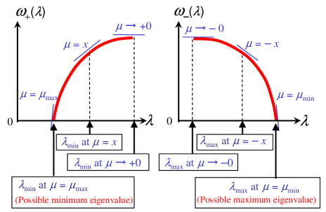
Figure 1: Schematic picture of entropy curve and relationship to parameter μ𝜇\mu.

The relationships among μ𝜇\mu, λ𝜆\lambda, and ω±subscript𝜔plus-or-minus{\omega}_{\pm} are illustrated in Fig. 1. Entropy densities ω+subscript𝜔{\omega}_{+} and ωsubscript𝜔{\omega}_{-} are convex increasing and decreasing functions of λ𝜆\lambda, respectively. According to eq. (15), the value of λ𝜆\lambda at μ𝜇\mu represents the point where the gradient of ω±subscript𝜔plus-or-minus{\omega}_{\pm} equals μ𝜇\mu. By definition, negative entropy values are not allowed, and ω±(λ|𝑨;ρ)<0subscript𝜔plus-or-minusconditional𝜆𝑨𝜌0{\omega}_{\pm}(\lambda|\bm{A};\rho)<0 implies that no 𝒄𝒄\bm{c} simultaneously satisfies both Λ±(𝒄|𝑨)=λ/2subscriptΛplus-or-minusconditional𝒄𝑨𝜆2\Lambda_{\pm}(\bm{c}|\bm{A})=\lambda/2 and ici=Nρsubscript𝑖subscript𝑐𝑖𝑁𝜌\sum_{i}c_{i}=N\rho. Therefore, the λ±superscriptsubscript𝜆plus-or-minus\lambda_{\pm}^{*} that produces ω±(λ±|𝑨;ρ)=0subscript𝜔plus-or-minusconditionalsuperscriptsubscript𝜆plus-or-minus𝑨𝜌0{\omega}_{\pm}(\lambda_{\pm}^{*}|\!\bm{A};\rho)\!\!=\!\!0 is the possible minimum or maximum eigenvalue. Hence, eqs. (11-12) give us

λmin(𝑨;ρ)=λ+,λmax(𝑨;ρ)=λ,formulae-sequencesuperscriptsubscript𝜆min𝑨𝜌superscriptsubscript𝜆superscriptsubscript𝜆𝑨𝜌superscriptsubscript𝜆\displaystyle\lambda_{\rm min}^{*}(\bm{A};\rho)=\lambda_{+}^{*},~{}~{}\lambda_{\max}^{*}(\bm{A};\rho)=\lambda_{-}^{*}, (17)

which are the typical values for μ=μmax𝜇subscript𝜇max\mu=\mu_{\rm max} and μ=μmin𝜇subscript𝜇min\mu=\mu_{\rm min}, respectively (Fig. 1).

IV RS analysis for Gaussian random matrix

This section applies the methodology introduced in the previous section to the case in which components of 𝑨𝑨\bm{A} are independently generated using a Gaussian distribution with mean 0 and variance (Nα)1superscript𝑁𝛼1(N\alpha)^{-1}. In this case, ϕ(μ|𝑨;ρ)italic-ϕconditional𝜇𝑨𝜌\phi(\mu|\bm{A};\rho) and ω±(λ|𝑨;ρ)subscript𝜔plus-or-minusconditional𝜆𝑨𝜌{\omega}_{\pm}(\lambda|\bm{A};\rho) randomly fluctuate depending on 𝑨𝑨\bm{A}. However, for all ϵ>0italic-ϵ0\epsilon>0, the probability that deviation from the typical values, ϕ(μ;ρ)[ϕ(μ|𝑨;ρ)]Aitalic-ϕ𝜇𝜌subscriptdelimited-[]italic-ϕconditional𝜇𝑨𝜌𝐴\phi(\mu;\rho)\equiv[\phi(\mu|\bm{A};\rho)]_{A} and ω±(λ;ρ)[ω±(λ|𝑨;ρ)]Asubscript𝜔plus-or-minus𝜆𝜌subscriptdelimited-[]subscript𝜔plus-or-minusconditional𝜆𝑨𝜌𝐴{\omega}_{\pm}(\lambda;\rho)\equiv[{\omega}_{\pm}(\lambda|\bm{A};\rho)]_{A}, is larger than ϵitalic-ϵ\epsilon tends to vanish as N𝑁N\to\infty. Here, []Asubscriptdelimited-[]𝐴[\cdot]_{A} denotes the average of 𝑨𝑨\bm{A}. Therefore, typical properties can be characterized by evaluating the typical values, ϕ(μ;ρ)italic-ϕ𝜇𝜌\phi(\mu;\rho) and ω±(λ)subscript𝜔plus-or-minus𝜆{\omega}_{\pm}(\lambda), using the replica method with the identity [13, 14]:

[logf(𝑨)]A=limn0nlog[fn(𝑨)]A\displaystyle[\log f(\bm{A})]_{A}=\lim_{n\to 0}\frac{\partial}{\partial n}\log[f^{n}(\bm{A})]_{A} (18)

where f(𝑨)𝑓𝑨f(\bm{A}) is an arbitrary function. When both n𝑛n and m=μ/β𝑚𝜇𝛽m=\mu/\beta are positive integers, regarding 𝒄Zcm(𝒄,𝑨;β)δ(i=1NciNρ)subscript𝒄superscriptsubscript𝑍𝑐𝑚𝒄𝑨𝛽𝛿superscriptsubscript𝑖1𝑁subscript𝑐𝑖𝑁𝜌\sum_{\bm{c}}Z_{c}^{m}(\bm{c},\bm{A};\beta)\delta(\sum_{i=1}^{N}c_{i}-N\rho) in eq. (13) as f(𝑨)𝑓𝑨f(\bm{A}) leads us to express [fn(𝑨)]Asubscriptdelimited-[]superscript𝑓𝑛𝑨𝐴[f^{n}(\bm{A})]_{A} as a summation/integration with respect to n𝑛n and nm𝑛𝑚nm replica variables {𝒄a}superscript𝒄𝑎\{\bm{c}^{a}\} and {𝒄a𝒖aσ}superscript𝒄𝑎superscript𝒖𝑎𝜎\{\bm{c}^{a}\circ\bm{u}^{a\sigma}\} (a{1,2,,n},σ{1,2,,m}formulae-sequence𝑎12𝑛𝜎12𝑚a\in\{1,2,\ldots,n\},\sigma\in\{1,2,\ldots,m\}), which can be evaluated by the saddle point method for N𝑁N\to\infty.

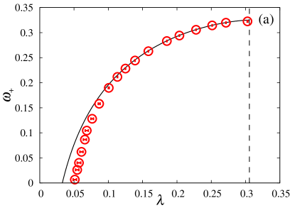
Refer to caption
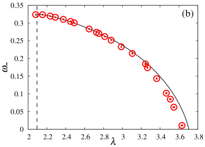
Refer to caption
Figure 2: Entropy curve for α=0.5𝛼0.5\alpha=0.5 and ρ=0.1𝜌0.1\rho=0.1 with (a) μ>0𝜇0\mu>0 and (b) μ<0𝜇0\mu<0. Circles denote EMC method results. Vertical lines represent (a) minimum and (b) maximum eigenvalues of MP distribution.

Under the replica symmetric (RS) assumption, in which the dominant saddle point is assumed to be invariant against any permutation of the replica indices a𝑎a and σ𝜎\sigma within each of their sets {1,2,,n}12𝑛\{1,2,\ldots,n\} and {1,2,,m}12𝑚\{1,2,\ldots,m\}, respectively, the resulting functional form of N1log[fn(𝑨)]AN^{-1}\log[f^{n}(\bm{A})]_{A} becomes extendable for non-integer n𝑛n and m𝑚m. Therefore, we insert the expression into eq. (13) employing the formula of eq. (18), which finally yields

ϕ(μ;ρ)=α2log{α+χ+μ(1q)}+α2log(α+χ)italic-ϕ𝜇𝜌𝛼2𝛼𝜒𝜇1𝑞𝛼2𝛼𝜒\displaystyle\phi(\mu;\rho)=-\frac{\alpha}{2}\log\{\alpha+\chi+\mu(1-q)\}+\frac{\alpha}{2}\log(\alpha+\chi)
αμq2{α+χ+μ(1q)}+Q^2q^12(1+χμ)+q^0q2+Kρ𝛼𝜇𝑞2𝛼𝜒𝜇1𝑞^𝑄2subscript^𝑞121𝜒𝜇subscript^𝑞0𝑞2𝐾𝜌\displaystyle-\frac{\alpha\mu q}{2\{\alpha+\chi+\mu(1-q)\}}+\frac{\hat{Q}}{2}-\frac{\hat{q}_{1}}{2}\Big{(}1+\frac{\chi}{\mu}\Big{)}+\frac{\hat{q}_{0}q}{2}+K\rho
+Dzlog{1+eKDyexp((q^1q^0y+q^0z)22Q^)},𝐷𝑧1superscript𝑒𝐾𝐷𝑦superscriptsubscript^𝑞1subscript^𝑞0𝑦subscript^𝑞0𝑧22^𝑄\displaystyle+\!\int\!\!Dz\log\Big{\{}1+e^{-K}\!\!\int\!\!Dy\exp\!\Big{(}\frac{(\sqrt{\hat{q}_{1}\!-\!\hat{q}_{0}}y\!+\!\sqrt{\hat{q}_{0}}z)^{2}}{2\hat{Q}}\Big{)}\Big{\}}, (19)

where {q,χ,Q^,q^0,q^1,K}𝑞𝜒^𝑄subscript^𝑞0subscript^𝑞1𝐾\{q,\chi,\hat{Q},\hat{q}_{0},\hat{q}_{1},K\} are determined to extremize the right hand side, and Dz=+dz2πexp(z2/2)𝐷𝑧superscriptsubscript𝑑𝑧2𝜋superscript𝑧22\int Dz=\int_{-\infty}^{+\infty}\frac{dz}{\sqrt{2\pi}}\exp(-z^{2}/2). The derivation of eq. (19) is shown in Appendix A. Entropy densities ω±(λ;ρ)subscript𝜔plus-or-minus𝜆𝜌{\omega}_{\pm}(\lambda;\rho) are derived by applying the inverse Legendre transformation to ϕ(μ;ρ)italic-ϕ𝜇𝜌\phi(\mu;\rho).

V Results

In Fig. 2, entropy densities ω±subscript𝜔plus-or-minus{\omega}_{\pm} with α=0.5𝛼0.5\alpha=0.5 and ρ=0.1𝜌0.1\rho=0.1 are shown for (a) μ<0𝜇0\mu<0 and (b) μ>0𝜇0\mu>0. Results of the exchange Monte Carlo (EMC) sampling are represented by circles, and the EMC procedure is summarized in Appendix B.

The values of λ𝜆\lambda when μ+0𝜇0\mu\to+0 and μ0𝜇0\mu\to-0, which are denoted using dashed lines, coincide with the respective minimum and maximum of the Marchenko-Pastur (MP) distribution’s support for the M×S𝑀𝑆M\times S Gaussian random matrix [15]. As the limit of |μ|0𝜇0|\mu|\to 0 corresponds to unbiased generation of M×S𝑀𝑆M\times S Gaussian random matrices, the coincidence theoretically supports the adequacy of our analysis. The slight discrepancy between the theoretical and EMC results in the entropy’s tails could be due to the insufficiency of the RS assumption. The convexity of our entropy suggests that the RS assumption exactly creates the entropy curve or extends it outward [16]. This is consistent with the EMC method’s result, which indicates that the exact entropy curve is inward when compared to that produced by the RS assumption. Therefore, the estimated zero-points, λmaxsuperscriptsubscript𝜆max\lambda_{\rm max}^{*} and λminsuperscriptsubscript𝜆min\lambda_{\rm min}^{*}, that are provided using the RS assumption, are meaningful upper and lower bounds, respectively, of the true values. We call them RS bounds.

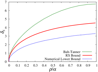
Fig. 3 compares our RS upper bound, Bah and Tanner’s upper bound [6], and the RIC numerically obtained lower bound [17]. In this example, the symmetric RIC is δSmaxsuperscriptsubscript𝛿𝑆max\delta_{S}^{\rm max}. Our analysis lowers the upper bound of the RIC, especially for a large ρ/α𝜌𝛼\rho/\alpha region. Over the entire parameter region, our estimates are consistent with the numerically obtained lower bound.
Refer to caption
Figure 3: Comparison of symmetric RIC for α=0.5𝛼0.5\alpha=0.5. Numerical lower bound is estimated for N=1000𝑁1000N=1000 and M=500𝑀500M=500.
Refer to caption
Figure 4: 0subscript0\ell_{0} and 1subscript1\ell_{1} limits given by RS RIC. Black lines represent Bah and Tanner’s results, denoted by BT.

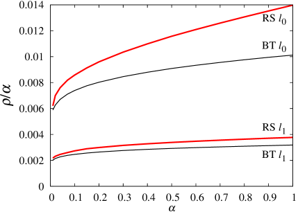
Fig. 4 shows the parameter region that mathematically supports 0subscript0\ell_{0} and 1subscript1\ell_{1} reconstruction according to Theorems 1 and 2. The region determined by the Bah and Tanner RIC is indicated using black lines. The RS bound of the RIC extends the region in which correct reconstruction is guaranteed, and further extension may be provided by taking the RSB into account.

VI Summary and conclusion

We proposed a theoretical scheme for the evaluation of restricted isometry constants. The problem was converted to the assessment of entropy density, and the possible maximum and minimum eigenvalues, which produce the RIC, are the entropy’s zero-points. Given a Gaussian random matrix, we computed the entropy density using the replica method under the replica symmetric ansatz and estimated the value of the RIC. Physically, it has meaning as a bound and is tighter than existing bounds. Numerical experiments using the EMC sampling support our analysis.

A more accurate evaluation of the RIC is possible if the RSB is taken into account. Our scheme is applicable to more general matrices than Gaussian random matrices as well.

Appendix A RS calculation of free entropy density

Identities

11\displaystyle 1 =𝑑q(a,σ)(b,τ)δ(q(a,σ)(b,τ)1Ni=1Nciacibuiaσuibτ),absentdifferential-dsuperscript𝑞𝑎𝜎𝑏𝜏𝛿superscript𝑞𝑎𝜎𝑏𝜏1𝑁superscriptsubscript𝑖1𝑁superscriptsubscript𝑐𝑖𝑎superscriptsubscript𝑐𝑖𝑏superscriptsubscript𝑢𝑖𝑎𝜎superscriptsubscript𝑢𝑖𝑏𝜏\displaystyle=\int dq^{(a,\sigma)(b,\tau)}\delta\Big{(}q^{(a,\sigma)(b,\tau)}-\frac{1}{N}\sum_{i=1}^{N}c_{i}^{a}c_{i}^{b}u_{i}^{a\sigma}u_{i}^{b\tau}\Big{)}, (20)

for all combinations of replica indices (a,σ)𝑎𝜎(a,\sigma) and (b,τ)𝑏𝜏(b,\tau) (a,b=1,2,,n;σ,τ=1,2,,m)formulae-sequence𝑎𝑏12𝑛𝜎𝜏12𝑚(a,b\!=\!1,2,\ldots,n;\sigma,\tau\!=\!1,2,\ldots,m), are employed in the saddle point assessment of ϕβ(n,m;ρ)N1log[(𝒄Zm(𝒄,𝑨;β)δ(i=1NciNρ))n]A\phi_{\beta}(n,m;\rho)\equiv N^{-1}\log[(\sum_{\bm{c}}Z^{m}(\bm{c},\bm{A};\beta)\delta(\sum_{i=1}^{N}c_{i}-N\rho))^{n}]_{A}. We assume that the dominant saddle point is of the replica symmetric form as

q(a,σ)(b,τ)={1fora=b,σ=τq1fora=b,στq0forab.superscript𝑞𝑎𝜎𝑏𝜏cases1formulae-sequencefor𝑎𝑏𝜎𝜏subscript𝑞1formulae-sequencefor𝑎𝑏𝜎𝜏subscript𝑞0for𝑎𝑏\displaystyle q^{(a,\sigma)(b,\tau)}=\begin{cases}1&\mbox{for}~{}a=b,~{}\sigma=\tau\\ q_{1}&\mbox{for}~{}a=b,~{}\sigma\neq\tau\\ q_{0}&\mbox{for}~{}a\neq b.\\ \end{cases} (21)

This means that when 𝑨𝑨\bm{A} is a Gaussian random matrix of mean 0 and variance (Nα)1superscript𝑁𝛼1(N\alpha)^{-1},

[sμaσsνbτ]A=α1δμν(δabδστ+q1δab(1δστ)+q0(1δab))subscriptdelimited-[]superscriptsubscript𝑠𝜇𝑎𝜎superscriptsubscript𝑠𝜈𝑏𝜏𝐴superscript𝛼1subscript𝛿𝜇𝜈subscript𝛿𝑎𝑏subscript𝛿𝜎𝜏subscript𝑞1subscript𝛿𝑎𝑏1subscript𝛿𝜎𝜏subscript𝑞01subscript𝛿𝑎𝑏\displaystyle[s_{\mu}^{a\sigma}s_{\nu}^{b\tau}]_{A}=\alpha^{-1}\delta_{\mu\nu}(\delta_{ab}\delta_{\sigma\tau}+q_{1}\delta_{ab}(1-\delta_{\sigma\tau})+q_{0}(1-\delta_{ab}))

holds, where sμaσiAμiciauiaσsuperscriptsubscript𝑠𝜇𝑎𝜎subscript𝑖subscript𝐴𝜇𝑖superscriptsubscript𝑐𝑖𝑎superscriptsubscript𝑢𝑖𝑎𝜎s_{\mu}^{a\sigma}\equiv\sum_{i}A_{\mu i}c_{i}^{a}u_{i}^{a\sigma}. Higher order correlations are negligible due to the central limit theorem, which indicates that sμaσsuperscriptsubscript𝑠𝜇𝑎𝜎s_{\mu}^{a\sigma} can be expressed as sμaσ=α1/2(1q1wμaσ+q1q0vμa+q0zμ)superscriptsubscript𝑠𝜇𝑎𝜎superscript𝛼121subscript𝑞1superscriptsubscript𝑤𝜇𝑎𝜎subscript𝑞1subscript𝑞0superscriptsubscript𝑣𝜇𝑎subscript𝑞0subscript𝑧𝜇s_{\mu}^{a\sigma}=\alpha^{-1/2}(\sqrt{1-q_{1}}w_{\mu}^{a\sigma}+\sqrt{q_{1}-q_{0}}v_{\mu}^{a}+\sqrt{q_{0}}z_{\mu}), where wμaσsuperscriptsubscript𝑤𝜇𝑎𝜎w_{\mu}^{a\sigma}, vμasuperscriptsubscript𝑣𝜇𝑎v_{\mu}^{a}, and zμsubscript𝑧𝜇z_{\mu} are i.i.d. Gaussian random variables of zero mean and unit variance. Replacing []Asubscriptdelimited-[]𝐴[\cdot]_{A} with average with respect to these Gaussain variables, the saddle point evaluation offers an expression of ϕβ(m,ρ)limn0nϕβ(n,m;ρ)subscriptitalic-ϕ𝛽𝑚𝜌subscript𝑛0𝑛subscriptitalic-ϕ𝛽𝑛𝑚𝜌\phi_{\beta}(m,\rho)\equiv\lim_{n\to 0}\frac{\partial}{\partial n}\phi_{\beta}(n,m;\rho), as

ϕβ(m;ρ)=m(Q~+q~1q1)m2(q~1q1q~0q0)2+DzlogΞβ(z)subscriptitalic-ϕ𝛽𝑚𝜌𝑚~𝑄subscript~𝑞1subscript𝑞1superscript𝑚2subscript~𝑞1subscript𝑞1subscript~𝑞0subscript𝑞02𝐷𝑧subscriptΞ𝛽𝑧\displaystyle\phi_{\beta}(m;\!\rho)\!=\!\frac{m(\tilde{Q}\!+\!\tilde{q}_{1}q_{1})\!-\!m^{2}(\tilde{q}_{1}q_{1}\!-\!\tilde{q}_{0}q_{0})}{2}\!+\!\!\int\!\!Dz\log\!\Xi_{\beta}(z)
+α[m2log(1+β(1q1)α)12log(1+μ(q1q0)α+β(1q1))\displaystyle+\alpha\Big{[}-\frac{m}{2}\log\!\Big{(}1\!+\!\frac{\beta(1-q_{1})}{\alpha}\Big{)}\!-\!\frac{1}{2}\log\Big{(}1\!+\!\frac{\mu(q_{1}-q_{0})}{\alpha\!+\!\beta(1-q_{1})}\Big{)}
μq02{α+β(1q1)+μ(q1q0)}]+Kρ,\displaystyle\hskip 28.45274pt-\frac{\mu q_{0}}{2\{\alpha+\beta(1-q_{1})+\mu(q_{1}-q_{0})\}}\Big{]}+K\rho, (22)

where

Ξβ(z)=1+subscriptΞ𝛽𝑧limit-from1\displaystyle\Xi_{\beta}(z)\!=\!1+ eK(Q~+q~1)m/2Dyexp(m(q~1q~0y+q~0z)22(Q~+q~1))superscript𝑒𝐾superscript~𝑄subscript~𝑞1𝑚2𝐷𝑦𝑚superscriptsubscript~𝑞1subscript~𝑞0𝑦subscript~𝑞0𝑧22~𝑄subscript~𝑞1\displaystyle\frac{e^{-K}}{(\tilde{Q}+\tilde{q}_{1})^{m/2}}\!\int\!\!Dy\exp\!\Big{(}\frac{m(\sqrt{\tilde{q}_{1}\!-\!\tilde{q}_{0}}y\!+\!\sqrt{\tilde{q}_{0}}z)^{2}}{2(\tilde{Q}+\tilde{q}_{1})}\Big{)}

and Q~~𝑄\tilde{Q}, K𝐾K, q~1subscript~𝑞1\tilde{q}_{1} and q~0subscript~𝑞0\tilde{q}_{0} are conjugate variables for the integral representations of delta functions in eq. (10), eq. (13) and eq. (20), respectively. Eq. (22) yields the free entropy density as ϕ(μ;ρ)=limβϕβ(μ/β,ρ)italic-ϕ𝜇𝜌subscript𝛽subscriptitalic-ϕ𝛽𝜇𝛽𝜌\phi(\mu;\rho)=\lim_{\beta\to\infty}\phi_{\beta}(\mu/\beta,\rho), in which the variables scale so that Q^m(Q~+q~1)^𝑄𝑚~𝑄subscript~𝑞1\hat{Q}\equiv m(\tilde{Q}+\tilde{q}_{1}), q^1m2q~1subscript^𝑞1superscript𝑚2subscript~𝑞1\hat{q}_{1}\equiv m^{2}\tilde{q}_{1}, q^0m2q~0subscript^𝑞0superscript𝑚2subscript~𝑞0\hat{q}_{0}\equiv m^{2}\tilde{q}_{0}, and χβ(1q1)𝜒𝛽1subscript𝑞1\chi\equiv\beta(1-q_{1}) become O(1)𝑂1O(1). This gives the expression of eq. (19).

The variables {χ,q0,Q^,q^1,q^0,K}𝜒subscript𝑞0^𝑄subscript^𝑞1subscript^𝑞0𝐾\{\chi,q_{0},\hat{Q},\hat{q}_{1},\hat{q}_{0},K\} are determined by extremization conditions of the free entropy density eq. (19),

χ𝜒\displaystyle\chi =μρQ^absent𝜇𝜌^𝑄\displaystyle=\frac{\mu\rho}{\hat{Q}} (23)
q𝑞\displaystyle q =Dz{Ξ(z)1Ξ(z)q^0zQ^Δ^}2absent𝐷𝑧superscriptΞ𝑧1Ξ𝑧subscript^𝑞0𝑧^𝑄^Δ2\displaystyle=\int Dz\Big{\{}\frac{\Xi(z)-1}{\Xi(z)}\frac{\sqrt{\hat{q}_{0}}z}{\hat{Q}-\hat{\Delta}}\Big{\}}^{2} (24)
11\displaystyle 1 =DzΞ(z)1Ξ(z)(Δ^Q^(Q^Δ^)+q^0z2(Q^Δ^)2)absent𝐷𝑧Ξ𝑧1Ξ𝑧^Δ^𝑄^𝑄^Δsubscript^𝑞0superscript𝑧2superscript^𝑄^Δ2\displaystyle=\int Dz\frac{\Xi(z)-1}{\Xi(z)}\Big{(}\frac{\hat{\Delta}}{\hat{Q}(\hat{Q}-\hat{\Delta})}+\frac{\hat{q}_{0}z^{2}}{(\hat{Q}-\hat{\Delta})^{2}}\Big{)} (25)
ρ𝜌\displaystyle\rho =DzΞ(z)1Ξ(z)absent𝐷𝑧Ξ𝑧1Ξ𝑧\displaystyle=\int Dz\frac{\Xi(z)-1}{\Xi(z)} (26)
Δ^^Δ\displaystyle\hat{\Delta} =αμ2(1q)(α+χ){α+χ+μ(1q)}absent𝛼superscript𝜇21𝑞𝛼𝜒𝛼𝜒𝜇1𝑞\displaystyle=\frac{\alpha\mu^{2}(1-q)}{(\alpha+\chi)\{\alpha+\chi+\mu(1-q)\}} (27)
q^0subscript^𝑞0\displaystyle\hat{q}_{0} =αμ2q{α+χ+μ(1q)}2absent𝛼superscript𝜇2𝑞superscript𝛼𝜒𝜇1𝑞2\displaystyle=\frac{\alpha\mu^{2}q}{\{\alpha+\chi+\mu(1-q)\}^{2}} (28)

where q=q0𝑞subscript𝑞0q=q_{0}, Δ^=q^1q^0^Δsubscript^𝑞1subscript^𝑞0\hat{\Delta}=\hat{q}_{1}-\hat{q}_{0}, and Ξ(z)=limβΞβ(z)Ξ𝑧subscript𝛽subscriptΞ𝛽𝑧\Xi(z)=\lim_{\beta\to\infty}\Xi_{\beta}(z).

Appendix B Monte Carlo sampling for RIC estimation

We employ the exchange Monte Carlo (EMC) sampling [9] in order to numerically compute the free entropy density ϕ(μ|𝑨;ρ)italic-ϕconditional𝜇𝑨𝜌\phi(\mu|\bm{A};\rho) and obtain the entropy density avoiding the trap of metastable states. In the EMC approach, we prepare k𝑘k systems, which have the same configuration of 𝑨𝑨\bm{A}, and assign configuration 𝒄i𝒄Ssubscript𝒄𝑖subscript𝒄𝑆\bm{c}_{i}\in\bm{c}_{S} and parameter μisubscript𝜇𝑖\mu_{i} to each system i=1,,k𝑖1𝑘i=1,\cdots,k. The signs of {μi}subscript𝜇𝑖\{\mu_{i}\} are set to be the same. Each step of the EMC process updates 𝒄isubscript𝒄𝑖\bm{c}_{i} within each system, and attempts exchanges between configurations 𝒄isubscript𝒄𝑖\bm{c}_{i} and 𝒄i+1subscript𝒄𝑖1\bm{c}_{i+1}. The probability of transition from 𝒄isubscript𝒄𝑖\bm{c}_{i} to 𝒄isuperscriptsubscript𝒄𝑖\bm{c}_{i}^{\prime} is given by w(𝒄i,𝒄i)=min{exp(μiNΔi),1},𝑤subscript𝒄𝑖superscriptsubscript𝒄𝑖subscript𝜇𝑖𝑁subscriptΔ𝑖1w(\bm{c}_{i},\bm{c}_{i}^{\prime})=\min\{\exp(\mu_{i}N\Delta_{i}),1\}, where Δi=Λsgn(μi)(𝒄i|𝑨)Λsgn(μi)(𝒄i|𝑨)subscriptΔ𝑖subscriptΛsgnsubscript𝜇𝑖conditionalsubscript𝒄𝑖𝑨subscriptΛsgnsubscript𝜇𝑖conditionalsuperscriptsubscript𝒄𝑖𝑨\Delta_{i}=\Lambda_{{\rm sgn}(\mu_{i})}(\bm{c}_{i}|\bm{A})-\Lambda_{{\rm sgn}(\mu_{i})}(\bm{c}_{i}^{\prime}|\bm{A}). The probability of an exchange between systems 𝒄isubscript𝒄𝑖\bm{c}_{i} and 𝒄i+1subscript𝒄𝑖1\bm{c}_{i+1} is given by wexc(𝒄i,𝒄i+1)=min{exp(N(μiμi+1)Δi,i+1),1},subscript𝑤excsubscript𝒄𝑖subscript𝒄𝑖1𝑁subscript𝜇𝑖subscript𝜇𝑖1subscriptΔ𝑖𝑖11w_{\rm exc}(\bm{c}_{i},\bm{c}_{i+1})=\min\!\{\exp(N(\mu_{i}\!-\!\mu_{i+1})\Delta_{i,i+1}),1\}, in which Δi,i+1=Λsgn(μi)(𝒄i|𝑨)Λsgn(μi+1)(𝒄i+1|𝑨)subscriptΔ𝑖𝑖1subscriptΛsgnsubscript𝜇𝑖conditionalsubscript𝒄𝑖𝑨subscriptΛsgnsubscript𝜇𝑖1conditionalsubscript𝒄𝑖1𝑨\Delta_{i,i+1}\!=\!\Lambda_{{\rm sgn}(\mu_{i})}(\bm{c}_{i}|\bm{A})\!-\!\Lambda_{{\rm sgn}(\mu_{i+1})}(\bm{c}_{i+1}|\bm{A}). After sufficient updates, the entire k𝑘k-system is expected to converge to equilibrium distribution Ptot({𝒄i}|𝑨)i=1kexp{NμiΛsgn(μi)(𝒄i|𝑨)}proportional-tosubscript𝑃totconditionalsubscript𝒄𝑖𝑨superscriptsubscriptproduct𝑖1𝑘𝑁subscript𝜇𝑖subscriptΛsgnsubscript𝜇𝑖conditionalsubscript𝒄𝑖𝑨P_{\rm tot}(\{\bm{c}_{i}\}|\bm{A})\propto\prod_{i=1}^{k}\exp\{-N\mu_{i}\Lambda_{{\rm sgn}(\mu_{i})}(\bm{c}_{i}|\bm{A})\}.

The density of states W±(λ|𝑨;ρ)=𝒄𝒄Sδ(λ/2Λ±(𝒄|𝑨))subscript𝑊plus-or-minusconditional𝜆𝑨𝜌subscript𝒄subscript𝒄𝑆𝛿𝜆2subscriptΛplus-or-minusconditional𝒄𝑨W_{\pm}(\lambda|\bm{A};\rho)\!=\!\sum_{\bm{c}\in\bm{c}_{S}}\delta(\lambda/2-\Lambda_{\pm}(\bm{c}|\bm{A})) is obtained by applying the multihistogram method [18] using histgrams of Λ±subscriptΛplus-or-minus\Lambda_{\pm} obtained by EMC sampling. Finally, the free entropy density is calculated:

ϕ(μ|𝑨;ρ)=𝑑λWsgn(μ)(λ|𝑨;ρ)exp(Nμλ/2),italic-ϕconditional𝜇𝑨𝜌differential-d𝜆subscript𝑊sgn𝜇conditional𝜆𝑨𝜌𝑁𝜇𝜆2\displaystyle\phi(\mu|\bm{A};\rho)=\int d\lambda W_{{\rm sgn}(\mu)}(\lambda|\bm{A};\rho)\exp(-N\mu\lambda/2), (29)

and the entropy density is derived by applying the inverse Legendre transformation to eq. (29).

Acknowledgment

The authors would like to thank Tomoyuki Obuchi for his helpful comments and discussions. This work was partially supported by the RIKEN SPDR fellowship and by KAKENHI No. 26880028 (AS), and KAKENHI No. 25120013 (YK).

References

  • [1] H. Nyquist, Trans. AIEE 47, 617 (1928).
  • [2] D. D. Lustig and J. Pauly, Magnet. Reson. Med. 58 (6), 1182–1195 (2007).
  • [3] J. Bobin et al., IEEE J. Sel. Top. Signal Process. 2 (5), 718–726 (2008).
  • [4] E. Candès et al., IEEE Trans. Inform. Theory 52 (2), 489–509 (2006).
  • [5] D. Donoho, IEEE Trans. Inform. Theory 52 (4), 1289–1306 (2006).
  • [6] E. Candès and T. Tao, IEEE Trans. Inform. Theory 51 (12), 4203–4215 (2005).
  • [7] J. D. Blanchard et al., SIAM Rev. 53 (1), 105–125 (2011).
  • [8] B. Bah, and J. Tanner, SIAM J. Matrix Anal. & Appl. 31 (5), 2882–2898 (2010).
  • [9] K. Hukushima, and K. Nemoto, J. Phys. Soc. Jpn, 65, 1604–1608 (1996).
  • [10] D. Donoho and Y. Tsaig, Signal Process. 86 (3), 549–581 (2006).
  • [11] S. Foucart and M.-J. Lai, Appl. Comput. Harmon. Anal. 26 (3), 395–407 (2009).
  • [12] R. Monasson and D. O’Kane, Europhys. Lett. 27 (2), 85–90 (1994).
  • [13] M. Me´´e\acute{\mbox{e}}zard et al., Spin Glass Theory and Beyond, (World Sci. Pub., 1987).
  • [14] H. Nishimori, Statistical Physics of Spin Glasses and Information Processing: An Introduction, (Oxford Univ. Pr., 2001).
  • [15] V. A. Marchenko and L. A. Pastur, Mat. Sb. (N. S.) 72 (114), 507–536 (1967).
  • [16] T. Obuchi et al., J. Phys. A: Math. Theor. 43, 485004 (28pp) (2010).
  • [17] C. Dossal et al., Linear Algebra Appl. 432, 1663–1679 (2010).
  • [18] A. M. Ferrenberg and R. H. Swendsen, Phys. Rev. Lett. 64, 1195–1198 (1989).