Fluctuations of ring polymers

Abstract

We present an exact solution for the distribution of sample averaged monomer to monomer distance of ring polymers. For non-interacting and weakly-interacting models these distributions correspond to the distribution of the area under the reflected Bessel bridge and the Bessel excursion respectively, and are shown to be identical in dimension $d\geq 2$. A symmetry of the problem reveals that dimension $d$ and $4-d$ are equivalent, thus the celebrated Airy distribution describing the areal distribution of the $d=1$ Brownian excursion describes also a polymer in three dimensions. For a self-avoiding polymer in dimension $d$ we find numerically that the fluctuations of the scaled averaged distance are nearly identical in dimension $d=2,3$ and are well described to a first approximation by the non-interacting excursion model in dimension $5$.

The statistical mechanics of polymers has been well studied for many years due both to the numerous practical applications of polymers as well as their many interesting properties. One signal finding is that the overall size of a polymer of length $N$ scales as $N^{\nu_{p}}$, where $\nu_{p}$ is a dimension dependent critical exponent. This is reflected in the behavior of various observables, such as the average end-to-end distance, and the radius of gyration ($R_{g}$) flory1969statistical ; de1979scaling . The scaling exponent is known to be sensitive to the excluded volume interaction applied to part or all of the monomers. Other geometrical constraints applied to the chain, such as cyclization (where the first monomer is connected to the last one), leading to a “ring” polymer, affect only the prefactor for these quantities. Ring polymers are commonly found in many biological systems e.g., bacterial and mitochondrial genomes, as well as DNA plasmids used in many molecular biology experiments alberts2002molecular . Recently, ring polymers were also studied in the context of a model for chromosome territories in the nucleus of eukaryotic cells halverson2012rheology .

The conformational fluctuations of some polymer models can be analyzed using the theory of random walks (RW) flory1969statistical ; de1979scaling . In particular, the fluctuations of the polymer size are of physical and biological importance. In the current paper we study the distribution of sample-averaged monomer-to-monomer distance of ring polymers, both for ideal, noninteracting polymers as well as for polymers with excluded volume. In particular, we exploit recent mathematical development on $d$ dimensional constrained Brownian motion (defined below) kessler2014distribution to find an exact expression for the distribution of sample averaged monomer to monomer distance for both ideal ring polymers and those with an additional excluded volume interaction applied at a single point. This observable yields insight on the sample averaged fluctuations of polymer sizes. An important ingredient of this calculation is the identification of the appropriate boundary conditions for the underlying equation, a variant of the Feynman-Kac equation, which depends on both the dimensionality and the interaction, and in turn yields a selection rule for the solution. The resulting distributions are then compared numerically to those measured in simulations for a ring polymer with full excluded volume constraints.

As we have noted, constrained random walks lie at the heart of our analysis. For rings, the primary constraint is that the path returns to the origin after $N$ steps. Statistics of such constrained one dimensional Brownian paths have been the subject of much mathematical research pitman1999brownian ; janson2007brownian ; perman1996distribution ; pitman2001distribution . These constrained paths have been given various names, depending on the additional constraints imposed. The basic case is that of a Brownian bridge where the return to the origin is the sole constraint. For a Brownian excursion, the path is also forbidden from reaching the origin in between. Majumdar and Comtet used Brownian excursions to determine statistical properties of the fluctuating Edwards Wilkinson interface in an interval majumdar2004exact ; majumdar2005airy . The focus of most previous work has been on the constrained one dimensional Brownian paths which describes inherently non-interacting systems (note that the problems of non-intersecting Brownian excursions tracy2007nonintersecting or vicious random walkers schehr2008exact in higher dimensions are exceptions). For the case of the fluctuations of ring polymers, we need to extend the theory of Brownian excursions and bridges to other dimensions. We address the influence of different kinds of interactions on the polymer structure, both analytically (for a single point interaction) and numerically (for a polymer with excluded volume interactions). These models yield rich physical behaviors and open new questions.

Polymer Models. We consider three lattice models of ring polymers with $N$ bonds, each of length $b$, in $d$ dimensions. The simplest polymer model is an “ideal ring” - a closed chain without excluded volume, where different monomers can occupy the same lattice site. While such a polymer does not exist in nature, its global behavior is the same as that of a polymer at the Flory $\theta$-temperature flory1969statistical . An ideal ring chain corresponds exactly to an unbiased RW in $d$ dimensions which starts and ends at the origin, i.e. a $d$-dimensional bridge. In the second model, the “weakly interacting ring polymer”, the first and last monomers are tied to the origin and no other monomer is allowed to occupy this lattice site. This case is equivalent to that of $d$-dimensional excursions. The third model is a ring polymer with excluded volume interactions, also called a self-avoiding walk (SAW). Further details on the polymer models and simulation methods are provided in the supplementary material (SM). We first consider the ideal and weakly interacting ring models, for which we can provide an analytic solution.

Bessel process. In the analogy between statistics of an ideal polymer and a RW, the position of the $i$th monomer, ${\bf r}_{i}$, corresponds to the position ${\bf r}_{i}$ of the random walker after $i$ time steps and $N$ is proportional to the total observation time. The Bessel process schehr2010extreme ; martin2011first describes the dynamics of the distance $r=|{\bf r}|$ from the origin of a Brownian particle in $d$ dimensions. This process is described by the following Langevin equation:

$$\dot{r}={(d-1)\over 2r}+\eta(t),$$ (1)

where $\eta(t)$ is Gaussian white noise satisfying $\langle\eta\rangle=0$ and $\langle\eta(t)\eta(t^{\prime})\rangle=\delta(t-t^{\prime})$. One may map the polymer models to the Bessel process using $\langle{\bf r}(t)^{2}\rangle=d\,t=Nb^{2}=\langle{\bf R}^{2}\rangle$, where ${\bf R}^{2}$ is the mean square end-to-end distance of an ideal linear polymer chain without constraints. In what follows we choose $b^{2}=d$ and $t=N$.

Bessel Excursions and Reflected Bridges. The process $r(t)$ with the additional constraint of starting and ending at the origin, is called a reflected (since $r\geq 0$) Bessel bridge. This process corresponds to an ideal (non-interacting) ring chain. Bessel excursions are paths still described by Eq. (1) however with the additional constraint that any path that reaches the origin (besides $t=0$ and $t=N$) is excluded. The Bessel excursion corresponds to what we have called the “weakly interacting” ring chain, where a multiple occupation of the origin is not allowed. The mapping of the polymer models to the Bessel process, allows us to extract statistical properties of the former with new tools developed in the stochastic community kessler2014distribution ; majumdar2005airy ; Barkai et al. [2014].

The Observable $A$. For a ring polymer, let ${\bf r}_{i}$ be the position of the $i$th monomer in space where $i=0..N$, and we place the origin at the position of the zeroth monomer, $r_{0}$. For the weakly interacting chain this monomer is also the excluding one. We study a new measure, $A$, for the size of a ring polymer, defined by

$$A=\sum_{i=0}^{N}|{\bf r}_{i}-{\bf r}_{0}|.$$ (2)

In the RW language, $A$ is the area under a random process, and hence is a random variable itself. Clearly $\bar{l}=A/N$ is the sample averaged distance of the monomers from the origin. Specifically, let the area under the random Bessel curve $r(t)$ be denoted by $A_{B}=\int_{0}^{t}r(t){\rm d}t$ (the subscript $B$ is for Bessel). More generally the mapping of the processes implies that in the limit of large $N$ the distribution of $A_{B}/\langle A_{B}\rangle$ is identical to the distribution of $A/\langle A\rangle$ (or $\bar{l}/\langle\bar{l}\rangle$), with the corresponding constraints.

Figure 1: (color online) Theoretical $P^{+}(A/\langle A\rangle)$ Eq. (10) in dimension $d=2,3,5$ nicely matches simulations of the ideal ring (IR) and the weakly interacting (WI) models, the exception being the weakly interacting model in $d=2$ due to critical slowing down (the simulations did not converge for $N=10^{6}$, see text). The theoretical curves (solid lines) for the two models are identical for $d\geq 2$. The $d=1$ WI theory is identical to the $d=3$ theory, which the simulation confirms. The SAW simulations in $d=2,3$ are practically indistinguishable from each other and from the theoretical curve corresponding to a noninteracting ring in dimension $d=5$.

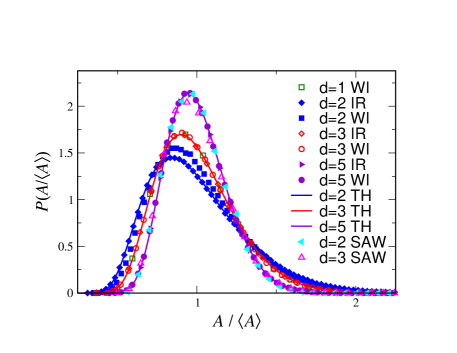
Numerical results. In Fig. 1 we plot the probability density function (PDF) of the scaled random variable $A/\langle A\rangle$. Both results of simulations and theory are presented, however at this stage let us focus on the main features as revealed in the simulations. For dimensions $d=2,\ldots,5$, there is a clear trend of narrowing of the PDF for increasing $d$. This trend is explained by examining Eq. (1): As $d$ increases, the noise term becomes negligible compared with the force term, resulting in smaller fluctuations and narrower tails. Against this expected trend are the results in $d=1$ for the weakly interacting model. As we will show analytically, the weakly interacting model in dimensions one and three surprisingly have the same distribution even though $d=1$ has a vanishing deterministic force term in Eq. (1) while for d = 3 the force is clearly not zero. In addition, we observe that for $d\geq 3$ the shape of the distribution of weakly interacting and ideal ring chains coincide, indicating that weak interactions are negligible (when $N\to\infty$). As we shall see, this is also observed in the theory. Indeed the theory discussed below suggests that these two distributions are already identical for $d=2$. However, since this is a critical dimension, due to extremely slow convergence, we don’t see this behavior in the simulations. This asymptotic convergence is logarithmic (see SM) and an $\varepsilon$ expansion shows that it is reminiscent of critical slowing down. As for the SAW polymer, we see that the fluctuations are considerably reduced compared to the other models. This is due to the fact that the number of configurations of a SAW polymer is smaller than for the other models, hence fluctuations are smaller. A striking observation is that the two and three dimensional SAW results are identical, both being equal to the simulations of the $d=5$ models. We now address these observations with theory.

Functionals of Constrained Bessel Processes. Our goal is to find the PDF $P(A_{B},t)$ of the functional $A_{B}=\int_{0}^{t}r(t){\rm d}t$ of the Bessel process, constrained to start and end at the origin. We show that the difference between the weakly interacting model (the Bessel excursion) and the ideal polymer (the reflected Bessel bridge) enters through the boundary condition in the Feynman-Kac type of equations describing these functionals. The choice of boundary condition turns out to be non-trivial and controls the solution. Other aspects of the solution follow the steps in kessler2014distribution .

It is useful to find first the Laplace transform of $P(A_{B},t)$, i.e., $\tilde{P}(s,t)=\int_{0}^{\infty}P(A_{B},t)\exp(-A_{B}s){\rm d}A_{B}$ to solve the equations, and invert $\tilde{P}(s,t)$ back to $P(A_{B},t)$. Let $G_{t}(r,A_{B}|r_{0})$ be the joint PDF of the random pair $(r,A_{B})$ with initial condition $G_{0}(r,A_{B}|r_{0})=\delta(A_{B})\delta(r-r_{0})$ and $\tilde{G}=\tilde{G}_{t}(r,s|r_{0})$ its Laplace pair. The modified Feynman-Kac equation reads carmi2011fractional :

$${1\over 2}\left[{\partial^{2}\over\partial r^{2}}+{\partial\over\partial r}{1-d\over r}\right]\tilde{G}-sr\tilde{G}={\partial\over\partial t}\tilde{G}.$$ (3)

with $\tilde{G}|_{t=0}=\delta(r-r_{0})$ and $r_{0}$ a cutoff which is eventually taken to zero. For $d=1$, the second term on the right hand side vanishes, and we get the celebrated Feynman-Kac equation corresponding to Brownian functionals brownianfuncMaj . The third linear term $-sr\tilde{G}$ stems from the choice of our observable, namely our functional $A_{B}$ is linear in $r$ carmi2011fractional . Since we are describing a ring polymer, the Bessel process must start and end on the origin, and so, following majumdar2004exact , we need to calculate

$$\tilde{P}(s,t)=\lim_{r=r_{0}\rightarrow 0}{\tilde{G}_{t}(r,s|r_{0})\over\tilde{G}_{t}(r,0|r_{0})}.$$ (4)

The denominator gives the proper normalization condition.

The first step in the calculation is to perform a similarity transformation:

$$\tilde{G}_{t}(r,s|r_{0})=\left({r\over r_{0}}\right)^{{d-1\over 2}}\widetilde{K}_{t}(r,s|r_{0}).$$ (5)

Using Eq. (3), $\tilde{K}_{t}(r,s|r_{0})$ is the imaginary time propagator of a Schrödingier operator:

$$\hat{H}\widetilde{K}_{t}(r,s|r_{0})+{\partial\over\partial t}\tilde{K}_{t}(r,s|r_{0})=\delta(r-r_{0})\delta(t)$$ (6)

with the effective Hamiltonian:

$$\hat{H}=-{1\over 2}{\partial^{2}\over\partial r^{2}}+{(d-2)^{2}-1\over 8r^{2}}+sr.$$ (7)

The effective Hamiltonian reveals a subtle symmetry, namely two systems in dimensions $d_{1}$ and $d_{2}$ satisfying $d_{1}+d_{2}=4$ behave identically. Note that this symmetry is not affected by the choice of functional (or observable) since the latter only modifies the last term in $\hat{H}$. This explains the identity of the $d=1$ and $d=3$ PDFs noted earlier.

Boundary Conditions for Ideal and Weakly Interacting Models. The solution of Eq. (6)

$$\widetilde{K}_{t}(r,s|r_{0})=\sum_{k}\phi_{k}(r)\phi_{k}(r_{0})e^{-\lambda_{k}t}$$ (8)

is constructed kessler2014distribution from the eigenfunctions $\phi_{k}$ of $\hat{H}$ where $\lambda_{k}$ is the $k$th eigenvalue and the normalization condition is $\int_{0}^{\infty}\phi_{k}^{2}(r){\rm d}r=1$. The subtle point in the analysis is the assignment of the appropriate boundary condition corresponding to the underlying polymer models we consider. The eigenfunctions at small $r$ exhibit one of two behaviors:

$$\phi^{+}_{k}\sim d^{+}_{k}r^{{1+|2-d|\over 2}}\ \ \mbox{or}\ \ \ \phi^{-}_{k}\sim d^{-}_{k}r^{{1-|2-d|\over 2}}.$$ (9)

From the normalization condition, the $\phi^{-}$ solution cannot be valid for $d\geq 4$ and $d\leq 0$. For the critical dimension $d=2$ the two solutions are: $\phi^{+}_{k}\sim d^{+}_{k}r^{{1\over 2}}\ \ \mbox{or}\ \ \ \phi^{-}_{k}\sim d^{-}_{k}r^{{1\over 2}}\ln r$. We now solve the problem for the two boundary conditions and then show how to choose the relevant one for the physical models under investigation.

The distribution of $A/\langle A\rangle$. Following the Feynman-Kac formalism described above and performing the inverse Laplace transform  kessler2014distribution , we find two solutions for the PDF of the scaled variable $\chi\equiv A/\langle A\rangle$

$$p^{\pm}(\chi) =-\frac{\Gamma(1\pm|\alpha|)}{2\pi\chi}\left(\frac{4}{(\sqrt{2}c_{\pm}\chi)^{2/3}}\right)^{\pm|\alpha|+1}$$

$$\times\sum_{k=0}^{\infty}[\tilde{d}^{\pm}_{k}]^{2}\bigg{[}\Gamma\left(\frac{5}{3}\pm|\nu|\right)\sin\left(\pi\frac{2\pm 3|\nu|}{3}\right){}_{2}F_{2}\left(\frac{8}{6}\pm\frac{|\nu|}{2},\frac{5}{6}\pm\frac{|\nu|}{2};\frac{1}{3},\frac{2}{3};-\frac{2\lambda_{k}^{3}}{27(c_{\pm}\chi)^{2}}\right)$$

$$-\frac{\lambda_{k}}{(\sqrt{2}c_{\pm}\chi)^{2/3}}\Gamma\left(\frac{7}{3}\pm|\nu|\right)\sin\left(\pi\frac{4\pm 3|\nu|}{3}\right){}_{2}F_{2}\left(\frac{7}{6}\pm\frac{|\nu|}{2},\frac{5}{3}\pm\frac{|\nu|}{2};\frac{2}{3},\frac{4}{3};-\frac{2\lambda_{k}^{3}}{27(c_{\pm}\chi)^{2}}\right)$$

$$+\frac{1}{2}\left(\frac{\lambda_{k}}{(\sqrt{2}c_{\pm}\chi)^{2/3}}\right)^{2}\Gamma\left(3\pm|\nu|\right)\sin\left(\pm\pi|\nu|\right){}_{2}F_{2}\left(2\pm\frac{|\nu|}{2},\frac{3}{2}\pm\frac{|\nu|}{2};\frac{4}{3},\frac{5}{3};-\frac{2\lambda_{k}^{3}}{27(c_{\pm}\chi)^{2}}\right)\bigg{]}.$$ (10)

The solution is independent of $N$ and valid in the limit of $N\to\infty$. Here, $|\alpha|=|d-2|/2$, $|\nu|=2|\alpha|/3$, and ${}_{2}F_{2}(\cdot)$ refers to the generalized hypergeometric functions. The supplementary material provides a list of $\lambda_{k}$ and $d_{k}$ values for $d=1,\ldots 4$. For $d=1$ the solution agrees with the known resultsmajumdar2004exact ; majumdar2005airy ; shepp1982integral ; knight2000moments , where the $+$ solution is the celebrated Airy distribution majumdar2004exact ; majumdar2005airy . The average of $A$ is

$$\langle A\rangle^{\pm}=c_{\pm}N^{3/2},\ \ c_{\pm}={\pi\Gamma\left(\pm{\left|2-d\right|\over 2}+{3\over 2}\right)\over 4\sqrt{2}\Gamma\left(\pm{|2-d|\over 2}+1\right)}.$$ (11)

The $+$ solution was previously presented in a slightly different form in kessler2014distribution and here the question is how to choose the solution for the corresponding polymer models. Clearly, for $d=2$, $\langle A\rangle^{+}=\langle A\rangle^{-}$, indicating that this is a critical dimension. Further $\langle A\rangle^{+}$ in $1$ and $3$ dimensions are identical and so is $\langle A\rangle^{-}$ as the result of the symmetry around $d=2$ in Eq. (7). The scaling $\langle A\rangle\propto N^{3/2}$ is expected since $r$ scales with the square root of $N$ as for Brownian motion, so the integral over the random processes $r$ scales like $N^{3/2}$.

We investigate the physical interpretation of the two possible boundary conditions. A mathematical classification of boundary conditions was provided in pitman1982decomposition ; martin2011first and here we find the physical situations where these conditions apply. We examine the behavior of the probability current associated with the $k^{\mathit{th}}$ mode: $J^{\pm}_{k}=-\frac{1}{2}\phi_{k}^{\pm}(r_{0})\left((r^{(d-1)/2}\phi_{k}^{\pm}(r))^{\prime}+(1-d)r^{(d-1)/2}\phi_{k}^{\pm}(r)/r\right)$ for $r$ near the boundary $r_{0}\to 0$ in dimension $d$. The analysis is summarized in Table 1. We see that in dimension two and higher, the current on the origin is either zero or positive. A positive current at the boundary means that probability is flowing into the system, which is an unphysical situation in our system. Hence we conclude that in dimension two and higher, the $-$ solution is not relevant. This implies that statistics of excursion and reflected bridges (and equivalently, ideal and weakly interacting ring polymers) are identical for $d\geq 2$ and correspond to the $+$ solution.

$d$	$\phi_{k}^{+}$	$J_{k}^{+}$	$\phi_{k}^{-}$	$J_{k}^{-}$
$d=1$	$\phi_{k}^{+}\sim r$	$J_{k}^{+}<0$	$\phi_{k}^{-}\sim\textit{Const}$	$J_{k}^{-}=0$
$d=2$	$\phi_{k}^{+}\sim\sqrt{r}$	$J_{k}^{+}=0$	$\phi_{k}^{-}\sim\sqrt{r}\log r$	$J_{k}^{-}>0$
$d=3$	$\phi_{k}^{+}\sim r$	$J_{k}^{+}=0$	$\phi_{k}^{-}\sim\textit{Const}$	$J_{k}^{-}>0$

Table 1: Behavior of the probability eigenfunctions and probability currents in the proximity of the origin ($r=0^{+}$) for the $+/-$ solutions in different dimensions. A current $J^{-}>0$ on the origin is unphysical hence the critical dimension where local interactions are uniportant is $2$.

In Fig. 1 we compare the results of the simulations of the ideal and weakly interacting polymer models with our theoretical results for $P^{+}(A/\langle A\rangle)$, as given in Eq. (10). As noted above, for $d\geq 3$, we see that even for finite size chains the local interaction is not important, and that the theory and simulations perfectly match, while for $d=2$ there are strong finite size effects in the weakly interacting case.

Self-avoiding polymers. Extensive simulations of ring SAWs were performed on cubic lattices.   As has already been pointed out, the global expansion of a polymer is characterized by the exponent $\nu_{p}$. Since $A$ constitutes a measure of the overall size of a polymer, its behavior for large $N$ should follow $A\sim N^{\nu_{p}+1}$. For the ideal and weakly-interacting chains $\nu_{p}=1/2$, and $A\sim N^{3/2}$. For SAWs the exact value of the exponent depends on $d$, i.e., $\nu_{p}=\nu_{p}(d)$. $\nu_{p}=1,0.75$, and $0.5$ are known exactly for $d=1,2$, and $4$ nienhuis1982exact , respectively, while for $d=3$, $\nu_{p}$, based on renormalization group considerations and Monte Carlo simulations, is $\nu_{p}\simeq 0.588$. These prediction were extensively tested numerically for the observable of interest $A$ with a critical dimension of $d=4$, characterized by a very slow convergence of the weakly-interacting model (see SM).

While the scaling behavior of the SAW model is different from that of the other two models (as reflected in $\nu_{p}$), as we have noted, the scaled PDFs, $P(A/\langle A\rangle)$ are nevertheless similar. A striking observation is that the SAWs in $d=2$ and $3$ coincide to the precision of our measurements with the comparably narrow PDF of the $d=5$ non-interacting model, (see Fig. 1). That these distribution are narrower than the non-self-avoiding case can be qualitatively explained as follows: Since the interaction forbids many compact conformations, the fluctuations of the area become smaller. This is easily observed in the extreme case of a linear SAW in one dimension where only one conformation is allowed and the scaled PDF assumes the form of a $\delta$-function.

Discussion. The mapping of ring polymer models to the reflected Bessel bridge and excursion is very promising since it implies that not only the observable $A$ can be analytically computed, but also other measures of statistics of ring polymers. An example would be the maximal distance from one of the monomers to any other monomer, since that would relate to extreme value statistics of a correlated process. The famed Airy distribution describes both the one dimensional polymer, as well as the three dimensional one, due to the symmetry we have found in the underlying Hamiltonian. The case of $d=2$ is critical in the sense that interaction on the origin becomes negligible, though for finite size chains it is still important. Boundary conditions of the Feynman-Kac equation were related to physical models, which allowed as to select the solutions relevant for physical models. The SAW polymer exhibits interesting behavior; the distribution of $A/\langle A\rangle$ is identical (up to numerical precision) in dimension $2$ and $3$ and corresponds to the non-interacting models in dimension $5$. Further work on this observation is required.

Acknowledgments: This work is supported by the Israel Science Foundation (ISF).

SUPPLEMENTARY MATERIAL

Appendix A Ring Polymer Simulations in $d$ dimensions

A.1 Ideal and Weakly Interacting Polymers

In our simulations for the ideal and weakly-interacting ring polymers the chain is built of $N$ consecutive bonds on a lattice. In the $i$th step, the bond displacement is $\Delta r_{i,j}=\pm 1$ in each of the $d$ directions, $j=1,\ldots,d$, hence the bond length is $b=\sqrt{\sum_{j=1}^{d}(\Delta{r_{j}})^{2}}=\sqrt{d}$. For example, for $d=3$, starting from the origin ($i=0$) with first step of $\Delta\mathbf{r}=(+1,-1,+1)$ (yielding $b=\sqrt{3}$) we reach the lattice site $\mathbf{r}_{1}=(+1,-1,+1)$. For a second step of $\Delta\mathbf{r}=(-1,-1,-1)$ we end up at lattice site $\mathbf{r}_{2}=(0,-2,0)$ for the $i=2$ monomer.

In order to maintain the closure condition of the chain, we choose an array of length of $N$ with $N/2$ components of $(+1)$ and $N/2$ of $(-1)$ in each of the directions ($d$ such arrays), and then shuffle them for each direction separately. For each $i$, the components of our $d$ dimensional step are the $i$th values of these arrays. The sum of all of the displacements in each direction is then naturally zero so that the last monomer is always positioned at the origin. For the ideal chain model we built $10^{6}$ such conformations while for the weakly interacting we threw away all the conformations that crossed the origin prior to the final monomer. For each of the conformations we calculated $A=\sum_{i=0}^{N}|r_{i}-r_{0}|$, where $r_{0}=0$, and plotted the distribution of this parameter.

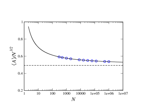
According to Eq. (11) in the paper, for $N\rightarrow\infty$ we have $\langle A\rangle=c_{\pm}N^{3/2}$. By this we can check the convergence of the simulations to the theory as a function of $N$. At the critical dimension, $d=2$ this convergence becomes very slow. In Fig. S1 we plot $\langle A\rangle/N^{3/2}$ for different $N$ values (in a logarithmic scale) in $d=2$, where $\langle A\rangle=c_{+}=0.4922$ is the theoretical value for $N\rightarrow\infty$. One can observe the very slow logarithmic convergence to this value.

Figure S1: (color online) $\langle A\rangle/N^{3/2}$ as a function of $N$ for the critical dimension $d=2$: weakly-interacting polymer simulations (blue circles) and the fitted curve of the function: $\langle A\rangle/N^{3/2}\simeq 0.497+0.544/\log(N)$. The black dashed line is the theoretical value of $c^{+}=0.4922$ for $N\rightarrow\infty$.

A.2 Self-Avoiding Ring Polymers

Monte Carlo (MC) simulations have been applied to self-avoiding ring polymer models Meirovitch [1988] on square, simple cubic, and $d=4$ hyper-cubic lattices. The polymer consists of $N$ monomers (and $N$ bonds), where the first monomer is attached to the origin of the coordinate system on the lattice, and the $N$th monomer is the nearest-neighbor to the origin. At step $j$ of the MC process, monomer $k$ ($1\leq k\leq N-1$) is selected at random (i.e., with probability $1/(N-1)$) and the segment of $m$ monomers following $k$ (i.e., $k+1,k+2,…,k+m$) become subject to change in the MC process; the rest of the chain (i.e., monomers $1$ to $k$ and $k+m+1$ to $N$) is held fixed (notice that if $k$ is at the end of the chain, $N-m+1<k\leq N-1$, $m$ decreases correspondingly from $m-1$ to $1$). Thus, this current segment is temporarily removed and a scanning procedure is used to calculate all the possible segment configurations of $m$ monomers satisfying the excluded volume interaction and the loop closure condition (i.e., the segment of $m$ monomers should start at $k$ and its last monomer, $k+m$ is a nearest neighbor to monomer $k+m+1$; notice that the initial segment configuration is generated as well). The segment configuration for step $j$ is chosen at random out of the set of $\mathcal{L}$ configurations generated by the scanning procedure and the MC process continues.

This process starts from a given ring configuration, whose transient influence is eliminated by a long initial simulation, which leads to typical equilibrium chain configurations. Then, every certain constant amount of MC steps the current ring configuration is stored in a file to create a final sample of $n$ rings from which the averages and fluctuations of the physical properties of interest are calculated. The segment sizes used are $m=10$ for the square lattice, $m=6$ for the simple cubic lattice, and $m=4$ for $d=4$. For each lattice several chain lengths, $N$ are studied.

Figure S2: (color online) Theoretical $P(A/\langle A\rangle)$ for reflected Bessel bridges and Bessel excursions for $d=4$ (black solid line) along with simulations of $d=4$ SAW for $N=200$ (blue diamonds), $N=400$ (green triangles), $N=800$ (blue circles), $N=1600$ (purple squares).

We calculated the averages of $R_{g}^{2}$,

$$R_{g}^{2}=\frac{1}{N}\sum_{i=0}^{N-1}{({\bf{r}}_{i}-{\bf{r}}_{c.m.})^{2}},$$ (S1)

where

$${\bf{r}}_{c.m.}\equiv\frac{1}{N}\sum_{i=0}^{N-1}{\bf{r}}_{i}$$ (S2)

and $A=\sum_{i=0}^{N-1}{|{\bf{r}}_{i}-{\bf{r}}_{0}|}$. For large $N$, $\langle R_{g}\rangle=\sqrt{\left\langle R_{g}^{2}\right\rangle}$ increases as $\sim N^{\nu_{p}}$ where $\nu_{p}$ is a critical exponent and as discussed in the text, ${\nu_{A}}={\nu_{p}+1}$. However, we are mainly interested in the fluctuations of $A$, i.e., in the shape of the scaled distribution of $A/\langle A\rangle$ for different $N$. To check the reliability of the simulations we provide in Table S1 the results obtained for $R_{g}$. The $\nu_{calculated}$ results for $d=2$ and $d=3$ are equal within the error bars to those of $\nu_{predicted}$ while for $d=4$ $\nu_{calculated}$ is too large due to a logarithmic correction to scaling, which would become insignificant only for much larger $N$. In fact, considering this correction in the analysis has led indeed to $\nu_{calculated}\simeq 0.5$. The same quality of results for ${\nu_{A}}$ has been obtained for the observable $A$ (where $\nu_{A}\simeq 1.5$ for $d=4$).

$d$	$N$ range	$\nu_{calculated}$	$\nu_{predicted}$
$2$	$200-1600$	$0.7507\pm 0.002$	$0.75$ (exact)
$3$	$60-1002$	$0.5890\pm 0.002$	$0.588$
$4$	$200-2560$	$0.525\pm 0.015$	$0.5$ (exact)

Table S1:

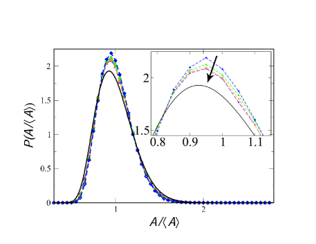
The $d=4$ SAW case is a critical one, since the critical exponent, $\nu_{p}$ for lower dimensions significantly differs from the $\nu_{p}=1/2$ of the non-interacting models, and for $d\geq 4$ the interactions become unimportant for $N\rightarrow\infty$. Hence, we expect $P(A/\langle A\rangle)$ of the $d=4$ SAW to coincide with that of the non-interacting model. However, for finite $N$ the interaction still has an effect on the distribution’s shape, and an even more pronounced one for ring polymers. For the values of $N$ we used in our SAW simulations the curve had not yet converged as can be seen in Fig. (S2). A downward trend of the curves towards that of the non-interacting case (i.e. towards convergence) can nevertheless be seen. A similar problem is not found for SAW in $d=2,3$ which are reported in the main text.

Appendix B Numeric values of $\lambda_{k}$ and $d_{k}$

The theoretical PDFs for different dimensions, presented in Eq. (10) in the paper, may be plotted using MATHEMATICA^®. In order to find the numerical coefficients $\lambda_{k}$ (eigenvalue) and $d_{k}$ (the normalization coefficient of the eigenfunction) values of the $k$th mode, we used the numerical method described in detail in Barkai et al. [2014]. In Table (S2) we present the values of the first few $\lambda_{k}$ and $d_{k}$ for different boundaries in different dimensions. We found that the first $7$ eigenvalues are usually sufficient for the evaluation of $P^{\pm}(A/\langle A\rangle)$.

Dimension	Value	$k=1$	$k=2$	$k=3$	$k=4$	$k=5$	$k=6$	$k=7$
$1,3$	$\lambda_{k}^{+}$	$2.3381$	$4.088$	$5.2056$	$6.7871$	$7.944$	$9.02265$	$10.040$
	$d_{k}^{+}$	$1$	$1$	$1$	$1$	$1$	$1$	$1$
$1$	$\lambda_{k}^{-}$	$1.0188$	$3.2482$	$4.8201$	$6.1633$	$7.3722$	$8.4885$	$9.5345$
	$d_{k}^{-}$	$0.99088$	$0.5550$	$0.4554$	$0.4241$	$0.3837$	$0.3663$	$0.3566$
$2$	$\lambda_{k}^{+}$	$1.738$	$3.671$	$5.170$	$6.475$	$7.658$	$8.755$	$9.787$
	$d_{k}^{+}$	$1.1391$	$0.9195$	$0.8386$	$0.7885$	$0.7597$	$0.7317$	$0.7109$
$4$	$\lambda_{k}^{+}$	$2.873$	$4.494$	$5.868$	$7.098$	$8.231$	$9.291$	$10.294$
	$d_{k}^{+}$	$0.7585$	$0.8807$	$0.9523$	$1.0047$	$1.0482$	$1.0820$	$1.1108$
$5$	$\lambda_{k}^{+}$	$3.362$	$4.885$	$6.208$	$7.406$	$8.516$	$9.558$	$10.547$
	$d_{k}^{+}$	$0.5187$	$0.6762$	$0.7838$	$0.8646$	$0.9405$	$1.0012$	$1.0531$

Table S2: The first $7$ eigenvalues, $\lambda_{k}$ and the corresponding numeric coefficients $d_{k}$ required for plotting the theoretical PDFs. The eigenvalues $\lambda_{k}^{+}$ of the $+$ solutions for $d=1$ and $d=3$ are the negatives of the zeros of the Airy function: $\textrm{Ai}(-\lambda_{k}^{+})=0$. The eigenvalues $\lambda_{k}^{-}$ of the $-$ solution are the negatives of the zeros of its derivative: $\textrm{Ai}^{\prime}(-\lambda_{k}^{-})=0$. The $d_{k}^{-}$ for $d=1$ are tabulated in Ref. Abramowitz and Stegun [1972].

References

- [1] P. J. Flory, Statistical Mechanics of Chain Molecules, Hanser, (Munich, 1989).
- [2] P. G. De Gennes, Scaling Concepts in Polymer Physics, Cornell Univ. Press, (Ithaca, 1979).
- [3] B. Alberts, et al., Molecular Biology of the Cell, 4th ed., Garland Science, (New York, 2002).
- [4] J. D. Halverson, G. S. Grest, A. Y. Grosberg and K. Kremer, Phys. Rev. Lett. 108, 038301 (2012).
- [5] D. A. Kessler, S. Medalion, and E. Barkai, J. Stat. Phys. 156, 686 (2014).
- [6] J. Pitman, Electron. J. Probab 4, 11 (1999). ‘
- [7] S. Janson, Probability Surveys 4, 80 (2007).
- [8] M. Perman and J. A. Wellner, Ann. Appl. Prob. 6, 1091 (1996).
- [9] J. Pitman and M. Yor, Ann. Prob. 29, 361 (2001).
- [10] S. N. Majumdar, and A. Comtet, Phys. Rev. Lett. 92, 225501 (2004)
- [11] S. N. Majumdar, and A. Comtet, J. Stat. Phys. 119, 707 (2005).
- [12] C. A. Tracy, and H. Widom, Ann. Appl. Prob. 17, 953 (2007).
- [13] G. Schehr, S. N. Majumdar, A. Comtet and J. Randon-Furling, Phys. Rev. Lett. 101, 150601 (2008).
- [14] G. Schehr, and P. Le Doussal, J. Stat. Mech: Theory and Expt. 2010(01), P01009 (2010).
- [15] E. Martin, U. Behn, and G. Germano, Phys. Rev. E 83, 051115 (2011).
- [16] E. Barkai, E. Aghion, and D. A. Kessler, Phys. Rev. X 4, 021036 (2014).
- [17] S. N. Majumdar, Current Science 89, 2076 (2005).
- [18] S. Carmi, and E. Barkai, Phys. Rev. E 84, 061104 (2011),
- [19] J. Pitman, and M. Yor Probability Theory and Related Fields 59, 425 (1982).
- [20] L. A. Shepp, Ann. Prob. 10, 234 (1982).
- [21] F. B. Knight, Intl. J. of Stoch. Analysis 13, 99 (2000).
- [22] B. Nienhuis, Phys. Rev. Lett. 49, 1062, (1982).
- Meirovitch [1988] H. Meirovitch, J. Chem. Phys. 89, 2514 (1988).
- Barkai et al. [2014] E. Barkai, E. Aghion, and D. Kessler, Physical Review X 4, 021036 (2014).
- Abramowitz and Stegun [1972] M. Abramowitz and I. A. Stegun, Handbook of mathematical functions: with formulas, graphs, and mathematical tables, 55 (Courier Dover Publications, 1972).