Wavelet estimation for operator fractional Brownian motion

Abstract

Operator fractional Brownian motion (OFBM) is the natural vector-valued extension of the univariate fractional Brownian motion. Instead of a scalar parameter, the law of an OFBM scales according to a Hurst matrix that affects every component of the process. In this paper, we develop the wavelet analysis of OFBM, as well as a new estimator for the Hurst matrix of bivariate OFBM. For OFBM, the univariate-inspired approach of analyzing the entry-wise behavior of the wavelet spectrum as a function of the (wavelet) scales is fraught with difficulties stemming from mixtures of power laws. The proposed approach consists of considering the evolution along scales of the eigenstructure of the wavelet spectrum. This is shown to yield consistent and asymptotically normal estimators of the Hurst eigenvalues, and also of the coordinate system itself under assumptions. A simulation study is included to demonstrate the good performance of the estimators under finite sample sizes.

1 Introduction

An ${\mathbb{R}}^{n}$-valued stochastic process $\{X(t)\}_{t\in{\mathbb{R}}}$ is said to be operator self-similar (o.s.s.) when its law scales according to a matrix (Hurst) exponent $H$, i.e.,

$$\{X(ct)\}_{t\in{\mathbb{R}}}\stackrel{{\scriptstyle\mathcal{L}}}{{=}}\{c^{H}X(t)\}_{t\in{\mathbb{R}}},\quad c>0,$$ (1.1)

where $c^{H}=\sum^{\infty}_{k=0}\log^{k}(c)H^{k}/k!$ and $\stackrel{{\scriptstyle\mathcal{L}}}{{=}}$ denotes the equality of finite-dimensional distributions. No specific assumption on the eigenstructure of $H$ is imposed, e.g., canonical vectors are not necessarily eigenvectors. The notion of operator self-similarity underpins the natural multivariate generalization of the univariate fractional Brownian motion (FBM): an operator fractional Brownian motion (OFBM) $B_{H}=\{B_{H}(t)\}_{t\in{\mathbb{R}}}$ is a proper Gaussian, o.s.s., stationary increment stochastic process. In this paper, we propose using the wavelet eigenstructure of OFBM to estimate $H$. The main motivation behind this methodology is to avoid the difficulties stemming from the extrapolation of univariate techniques to a multivariate context, where operator scaling laws such as (1.1) may arise.

Inferential theory for univariate self-similar processes now comprises a voluminous and well-established literature. A non-exhaustive list includes Fox and Taqqu (?) and Robinson (?, ?) on Fourier domain methods, and Wornell and Oppenheim (?), Flandrin (?), and Veitch and Abry (?) on wavelet domain methods, among many others. The multivariate framework evokes several applications where matrix-based scaling laws are expected to appear, such as in long range dependent time series (Marinucci and Robinson (?), Davidson and de Jong (?), Chung (?), Dolado and Marmol (?), Davidson and Hashimzade (?), Kechagias and Pipiras (?)) and queueing systems (Konstantopoulos and Lin (?), Majewski (?, ?), Delgado (?)). Like FBM in the univariate setting, OFBM is a natural starting point in the construction of estimators for operator self-similar processes due to its tight connection to stationary fractional processes and its being Gaussian (on the general theory of o.s.s. processes, see Laha and Rohatgi (?), Hudson and Mason (?), Maejima and Mason (?), Cohen et al (?)).

A characterization of the covariance structure of OFBM can be derived from stochastic integral representations. Under a mild condition on the eigenvalues of the exponent $H$ (see (2.9)), Didier and Pipiras (?) showed that any OFBM $B_{H}$ admits a harmonizable representation

$$\{B_{H}(t)\}_{t\in{\mathbb{R}}}\stackrel{{\scriptstyle{\mathcal{L}}}}{{=}}\Big{\{}\int_{{\mathbb{R}}}\frac{e^{itx}-1}{ix}(x^{-D}_{+}A+x^{-D}_{-}\overline{A})\widetilde{B}(dx)\Big{\}}_{t\in{\mathbb{R}}}$$ (1.2)

for some complex-valued matrix $A$. In (1.2), $x_{\pm}=\max\{\pm x,0\}$,

$$D=H-\frac{1}{2}\hskip 2.84526ptI,$$ (1.3)

and $\widetilde{B}(dx)$ is a complex-valued random measure such that $\widetilde{B}(-dx)=\overline{\widetilde{B}(dx)}$, $E\widetilde{B}(dx)\widetilde{B}(dx)^{*}=dx$, where $*$ represents Hermitian transposition. Expression (1.2) shows that the law of an OFBM can be fully described based on the scaling matrix $H$ and the spectral parameter $A$ (see Remark 2.1 on the parametrization).

Let $H=PJ_{H}P^{-1}$, $P\in GL(n,{\mathbb{C}})$, be the Jordan form of the Hurst parameter in (1.2) (see Section 2 for matrix notation). If $H$ is diagonal, then we can assume that $P$ takes the form of a scalar matrix $P=pI$, where $p\in{\mathbb{R}}$ and $I$ is the $n\times n$ identity matrix, and that $J_{H}=\textnormal{diag}(h_{1},\ldots,h_{n})$. In this case, (1.1) breaks down into simultaneous entry-wise expressions

$$\{X(ct)\}_{t\in{\mathbb{R}}}\stackrel{{\scriptstyle\mathcal{L}}}{{=}}\{(c^{h_{1}}X_{1}(t),\ldots,c^{h_{n}}X_{n}(t))^{*}\}_{t\in{\mathbb{R}}},\quad c>0.$$ (1.4)

Relation (1.4) is henceforth called entry-wise scaling. In particular, under (1.4) an OFBM is a vector of correlated FBM entries (Amblard et al. (?), Coeurjolly et al. (?)). Several estimators have been developed by building upon the univariate, entry-wise scaling laws, e.g., the Fourier-based multivariate local Whittle (e.g., Shimotsu (?), Nielsen (?)) and the multivariate wavelet regression (Wendt et al. (?), Amblard and Coeurjolly (?), Achard and Gannaz (?)). However, if $H$ is non-diagonal, i.e., if $P$ is not a scalar matrix, then the relation (1.1) mixes together the several entries of $X$. The estimation problem under a non-scalar $P$ turns out to be rather intricate and calls for the construction of methods that are multivariate from their inception.

Although the emergence of o.s.s. processes in applications is rightly expected – e.g., as functional weak limits of multivariate time series –, there is no specific reason to believe a priori that scaling laws occur predominantly entry-wise and exactly along the canonical axes. Indeed, this is palpably not true in several applications such as fractional blind-source separation (see Didier et al. (?)) and fractional cointegration (see Robinson (?) for a bivariate local Whittle estimator). The framework of multivariate mixed fractional time series subsumes both cases. Let $W=\{W_{t}\}_{t\in{\mathbb{Z}}}$ be an unobserved signal. To fix ideas suppose that the signal is an operator fractional Gaussian noise (OFGN), namely, it has the form $W_{t}=B_{H_{W}}(t)-B_{H_{W}}(t-1)$ with spectral parameter $A_{W}$ (see (1.2)). Further assume that $H_{W}=\textnormal{diag}(h_{1},\ldots,h_{n})$. The observed signal has the form $Y=\{Y_{t}\}_{t\in{\mathbb{Z}}}=\{PW_{t}\}_{t\in{\mathbb{Z}}}$, for a non-scalar, mixing matrix $P\in GL(n,{\mathbb{R}})$. Then, the mixed process $Y$ is another OFGN with parameters $H_{Y}=P\textnormal{diag}(h_{1},\ldots,h_{n})P^{-1}$ and $A_{Y}=PA_{W}$. In blind source separation, the entries of $W$ are uncorrelated, whereas in cointegration they are typically correlated.

From a mathematical standpoint, the mixing of scaling laws can be illustrated by means of the expression for the spectral density $f_{X}$ of an OFBM with Hurst parameter $H=P\textnormal{diag}(h_{1},h_{2})P^{-1}$, $0<h_{1}<h_{2}<1$, $P\in GL(2,{\mathbb{R}})$ (see condition (2.12)). For $M:=P^{-1}AA^{*}(P^{*})^{-1}\in M(n)$ (c.f. condition (2.11)) and $x>0$, the spectral density takes the form $\Big{(}f_{X}(x)_{ij}\Big{)}=x^{-D}AA^{*}x^{-D^{*}}$, where

$$f_{X}(x)_{11}=p^{2}_{11}m_{11}x^{-2d_{1}}+2p_{11}p_{12}m_{12}x^{-(d_{1}+d_{2})}+p^{2}_{12}m_{22}x^{-2d_{2}},$$

$$f_{X}(x)_{21}=p_{11}p_{21}m_{11}x^{-2d_{1}}+(p_{11}p_{22}+p_{12}p_{21})m_{12}x^{-(d_{1}+d_{2})}+p_{12}p_{22}m_{22}x^{-2d_{2}},$$

$$f_{X}(x)_{22}=p^{2}_{21}m_{11}x^{-2d_{1}}+2p_{21}p_{22}m_{12}x^{-(d_{1}+d_{2})}+p^{2}_{22}m_{22}x^{-2d_{2}},$$

and $d_{1}=h_{1}-1/2$, $d_{2}=h_{2}-1/2$ (see (LABEL:e:S=a(nu)HEW(j)a(nu)H*=(a_b_b_c)) for the analogous expression in the wavelet domain). The univariate-inspired approach of setting up a Fourier-domain log-regression – e.g., Whittle-type estimators – has to cope with the double-sided challenge of mixed power laws. On one hand, under mild assumptions on the amplitude coefficients, the dominant power law $x^{-2d_{2}}$ always prevails around the origin of the spectrum. On the other hand, and paradoxically, even if the estimation of $d_{2}$ is the target, the magnitude of the amplitude coefficients themselves can arbitrarily bias the estimate over finite samples by masking the dominant power law.

In this work, we build upon the wavelet analysis of ($n$-dimensional) OFBM to propose a novel wavelet-based estimation method for bivariate, and potentially multivariate, OFBM. The method yields the Hurst eigenvalues of $H$ and, under mild assumptions, also its eigenvectors when $P\in O(2)$. Its essential ingredient, and the main theme of this paper, is a change of perspective: instead of considering the entry-wise behavior of the wavelet spectrum as a function of wavelet scales, it draws upon the evolution along scales of the eigenstructure of the wavelet spectrum. This way, it avoids much of the difficulty associated with inference in the presence of mixed power laws, as we now explain.

For a wavelet function $\psi\in L^{2}({\mathbb{R}})$ with a number $N_{\psi}$ of vanishing moments (see (2.6)), the (normalized) vector wavelet transforms of OFBM is naturally defined as

$${\mathbb{R}}^{n}\ni D(2^{j},k)=2^{-j/2}\int_{{\mathbb{R}}}2^{-j/2}\psi(2^{-j}t-k)B_{H}(t)dt,\quad j\in{\mathbb{N}}\cup\{0\},\quad k\in{\mathbb{Z}},$$ (1.5)

provided the integral in (1.5) exists in an appropriate sense. The wavelet-domain process $\{D(2^{j},k)\}_{k\in{\mathbb{Z}}}$ is stationary in $k$ and o.s.s. in $j$ (Proposition 3.1). Moreover, whereas the original stochastic process $B_{H}(t)$ displayed fractional memory, the covariance between (multivariate) wavelet coefficients decays as a function of $|2^{j}k-2^{j^{\prime}}k^{\prime}|$ according to an inverse fractional power controlled by $N_{\psi}$ (Proposition 3.2). The wavelet spectrum (variance) at scale $j$ is the positive definite matrix

$$ED(2^{j},k)D(2^{j},k)^{*}=ED(2^{j},0)D(2^{j},0)^{*}=:EW(2^{j}),$$

and its natural estimator, the sample wavelet variance, is the matrix statistic

$$W(2^{j})=\frac{1}{K_{j}}\sum^{K_{j}}_{k=1}D(2^{j},k)D(2^{j},k)^{*},\quad K_{j}=\frac{\nu}{2^{j}},\quad j=j_{1},\ldots,j_{m},$$ (1.6)

for a dyadic total of $\nu$ (wavelet) data points. Within the bivariate framework, the univariate-like entry-wise scaling approach would consist of exploiting the behavior of each component $W(2^{j})_{i_{1},i_{2}}$, $i_{1},i_{2}=1,2$, of the sample wavelet transform $W(2^{j})$ as a function of the scales $2^{j}$. Apart from an amplitude effect, the entries are then controlled by the dominant Hurst eigenvalue $h_{2}$ (see expression (LABEL:e:Shat=a(nu)H_EW(j)_a(nu)H*=(a_b_b_c))). Figure 1, top panels, illustrates the fact that this precludes the estimation of $h_{1}$.

The proposed estimators of the Hurst eigenvalues $h_{1}$ and $h_{2}$ are

$$\widehat{h}_{1}(2^{j})=\frac{\log\lambda_{1}(2^{j})}{2\log(2^{j})},\quad\widehat{h}_{2}(2^{j})=\frac{\log\lambda_{2}(2^{j})}{2\log(2^{j})},$$ (1.7)

where $\lambda_{1}(2^{j})\leq\lambda_{2}(2^{j})$ are the eigenvalues of the positive definite symmetric matrix $W(2^{j})$ (see Definition 4.1 for the precise assumptions). However, as usual with operator self-similarity, the finite sample expressions for $\lambda_{1}(2^{j})$ and $\lambda_{2}(2^{j})$ themselves involve a mixture of distinct power laws $2^{j2h_{1}}$, $2^{j(h_{1}+h_{2})}$, $2^{j2h_{2}}$ ($h_{1}<h_{2}$). For this reason, one must take the limit at coarse scales, namely, the scale itself must go to infinity. It is a remarkable fact that the power law $2^{j2h_{1}}$ ends up prevailing in the expression for $\lambda_{1}(2^{j})$ (see Figure 1, bottom panels, and the striking contrast with the top panels; see Remark LABEL:r:motivation for a mathematically motivated, intuitive discussion). The convergence of (1.7) in turn allows for the convergence of associated sequences of eigenvectors when $P$ is orthogonal. Moreover, simulation studies show that the estimation procedure is accurate and computationally fast. The asymptotics are mathematically developed in two stages. In the first, the wavelet scales (octaves) are held fixed and the asymptotic distribution of the sample wavelet transform is obtained (Proposition 3.3 and Theorem 3.1). In the second, one takes the limit with respect to the scales themselves. However, the latter must go to infinity slower than the sample size, a feature that our estimators share with Fourier or wavelet-based semiparametric estimators in general (e.g., Robinson (?), Moulines et al. (?, ?, ?)).

Our results are related to the literature on the estimation of operator stable laws via eigenvalues and eigenvectors of sample quadratic forms (see Meerschaert and Scheffler (?, ?)). In this context, one encounters the same problem with the prevalence of some dominant power law (i.e., the tail exponent) in most directions. In Becker-Kern and Pap (?), a similar philosophy is applied in the time domain to produce one of the very few available estimators for authentic, mixed scaling o.s.s. processes of dimension up to 4. However, the asymptotics provided are restricted to consistency. In our work, the wavelet transform is the main tool for ensuring the consistency and asymptotic normality of the proposed estimators.

The paper is organized as follows. Section 2 contains the notation, assumptions and basic concepts. Section 3 is dedicated to the wavelet analysis of $n$-dimensional OFBM, as well as the asymptotics of the wavelet transform for fixed scales (most of the proofs can be found in Section LABEL:s:asympt_normality_fixed_scales). In Section 4, the estimation method for the Hurst exponent of bivariate OFBM is laid out in full detail and its asymptotics are established at coarse scales. Section LABEL:s:simulation_studies displays finite sample computational studies, including one of the performance of the estimators under blind source separation and cointegrated instances, with the purpose of illustrating the robustness of the estimators’ performance with respect to different parametric scenarios. The research contained in this paper leads to a number of interesting open questions, which are mentioned in Section LABEL:s:open. Among these is the extension of the consistency and asymptotic normality to any dimension $n\geq 3$, which will generally require dispensing with explicit formulas for eigenvalues and eigenvectors. The appendix contains several auxiliary mathematical results. In addition, in Section LABEL:s:discretized_wavelet, the performance of the estimators is established under the assumption that only discrete observations are available, instead of a full sample path as in (1.5).

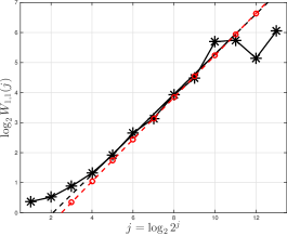
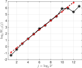
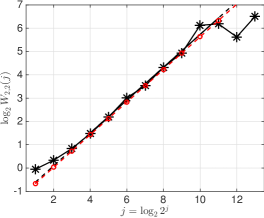
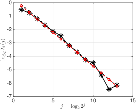
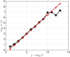
Figure 1: Entry-wise vs eigenvalue-based estimation. From one synthetic realization of OFBM, the top row displays (black solid lines with $\ast$), from left to right, $\log_{2}W(2^{j})_{1,1}$ vs $j$, $\log_{2}W(2^{j})_{1,2}$ vs $j$ and $\log_{2}W(2^{j})_{2,2}$ vs. $j$, on which the asymptotic behavior $j2h_{2}$ is superimposed (red dashed line with ‘o’). All auto- and cross-components are then driven by the dominant Hurst eigenvalue $h_{2}$, which precludes the estimation of the eigenvalue $h_{1}$. The first two bottom row plots display (black solid lines with $\ast$), from left to right, $\log_{2}\lambda_{1}(2^{j})$ vs $j$ and $\log_{2}\lambda_{2}(2^{j})$ vs $j$, with their respective asymptotic trends $j2h_{1}$ and $j2h_{2}$ superimposed (red dashed line with ‘o’). This demonstrates that both Hurst eigenvalues $h_{1}$ and $h_{2}$ can be estimated (see Section LABEL:s:entry-wise_vs_eigenvalue for the simulation details). The bottom right plot displays the increments of the generated OFBM.

2 Notation and assumptions

All through the paper, the dimension of OFBM is denoted by $n\geq 2$.

We shall use throughout the paper the following notation for finite-dimensional operators (matrices). All with respect to the field ${\mathbb{R}}$, $M(n)$ or $M(n,{\mathbb{R}})$ is the vector space of all $n\times n$ matrices (endomorphisms), $GL(n)$ or $GL(n,{\mathbb{R}})$ is the general linear group (invertible matrices, or automorphisms), $O(n)$ is the (orthogonal) group of matrices $O$ such that $OO^{*}=I=O^{*}O$ (i.e., the adjoint operator is the inverse), and ${\mathcal{S}}(n,{\mathbb{R}})$ is the space of symmetric matrices. We also write $I_{n}$ to indicate the dimension of the identity matrix $I$. A block-diagonal matrix with main diagonal blocks ${\mathcal{P}}_{1},\ldots,{\mathcal{P}}_{n}$ or $m$ times repeated diagonal block ${\mathcal{P}}$ is represented by

$$\textnormal{diag}({\mathcal{P}}_{1},\ldots,{\mathcal{P}}_{n}),\quad\textnormal{diag}_{m}({\mathcal{P}}),$$ (2.1)

respectively. The symbol $\|\cdot\|$ represents a generic matrix or vector norm. For $q\in{\mathbb{N}}$, the $l^{q}$ entry-wise norm of an $m\times n$ real-valued matrix $M$ is denoted by

$$\|M\|_{l^{q}}=\Big{(}\sum^{m}_{i_{1}=1}\sum^{n}_{i_{2}=1}|M_{i_{1},i_{2}}|^{q}\Big{)}^{1/q}$$ (2.2)

and $\|M\|_{l^{\infty}}=\sup_{i_{1},i_{2}}|M_{i_{1},i_{2}}|$. A generic matrix $M\in M(n,{\mathbb{C}})$ has real and imaginary parts $\Re(M)$ and $\Im(M)$, respectively. The functions

$$\pi_{i}(v),\pi_{i_{1},i_{2}}(M),\quad{\mathbf{v}}\in{\mathbb{R}}^{n},\quad M\in M(n,{\mathbb{R}}),$$ (2.3)

denote, respectively, the $i$-th projection (entry) of the vector ${\mathbf{v}}$ and the $(i_{1},i_{2})$-th projection (entry) of the matrix $M$, $i_{1},i_{2}=1,\ldots,n$. For $S=(s_{i_{1},i_{2}})_{i_{1},i_{2}=1,\ldots,n}\in{\mathcal{S}}(n,{\mathbb{R}})$, we define the operator

$$\textnormal{vec}_{{\mathcal{S}}}(S)=(s_{11},s_{12},\ldots,s_{1n};s_{22},\ldots,s_{2n};\ldots;s_{n-1,n-1},s_{n-1,n};s_{n,n})^{*}.$$ (2.4)

In other words, $\textnormal{vec}_{{\mathcal{S}}}(\cdot)$ vectorizes the upper triangular entries of the symmetric matrix $S$.

When establishing bounds, $C$ stands for a positive constant whose value can change from one line to the next. For a sequence of random vectors $\{X_{l},Y_{l}\}_{l\in{\mathbb{N}}}$, $P(Y_{l}=0)=0$, we write

$$X_{l}\stackrel{{\scriptstyle P}}{{\sim}}Y_{l}$$ (2.5)

to mean that $X_{l}/Y_{l}\stackrel{{\scriptstyle P}}{{\rightarrow}}1$, $l\rightarrow\infty$. Note that this does not imply that $\{X_{l},Y_{l}\}_{l\in{\mathbb{N}}}$ converges in probability. Relations of the type (2.5) will often appear in the proofs of the results in Section 4. We write ${\mathbf{X}}\stackrel{{\scriptstyle d}}{{=}}{\mathbf{Y}}$ when the random vectors ${\mathbf{X}}$ and ${\mathbf{Y}}$ have the same distribution.

All through the paper, we will make the following assumptions on the underlying wavelet basis. For this reason, such assumptions will be omitted in the statements.

Assumption $(W1)$: $\psi\in L^{1}({\mathbb{R}})$ is a wavelet function, namely,

$$\int_{{\mathbb{R}}}\psi^{2}(t)dt=1,\quad\int_{{\mathbb{R}}}t^{q}\psi(t)dt=0,\quad q=0,1,\ldots,N_{\psi}-1,\quad N_{\psi}\geq 2.$$ (2.6)

Assumption $(W2)$:

$$\textnormal{$\textnormal{supp}(\psi)$ is a compact interval}.$$ (2.7)

Assumption $(W3)$: there is $\alpha>1$ such that

$$\sup_{x\in{\mathbb{R}}}|\widehat{\psi}(x)|(1+|x|)^{\alpha}<\infty.$$ (2.8)

Under (2.6), (2.7) and (2.8), $\psi$ is continuous, $\widehat{\psi}(x)$ is everywhere differentiable and its first $N_{\psi}-1$ derivatives are zero at $x=0$ (see Mallat (?), Theorem 6.1 and the proof of Theorem 7.4).

Example 2.1

If $\psi$ is a Daubechies wavelet with $N_{\psi}$ vanishing moments, $\textnormal{supp}(\psi)=[0,2N_{\psi}-1]$ (see Mallat (?), Proposition 7.4).

Starting from the harmonizable representation (1.2), throughout the paper we will make the following assumptions on the OFBM $B_{H}=\{B_{H}(t)\}_{t\in{\mathbb{R}}}$.

Assumption (OFBM1): the eigenvalues (characteristic roots) $h_{k}$ of the matrix exponent $H$ satisfy

$$0<\Re(h_{k})<1,\quad k=1,\ldots,n.$$ (2.9)

Assumption (OFBM2):

$$\textnormal{$\Re(AA^{*})$ has full rank}.$$ (2.10)

The condition (2.9) generalizes the familiar constraint $0<H<1$ on the Hurst parameter of a FBM. As shown in Didier and Pipiras (?), it ensures the existence of the harmonizable representation (1.2). Also, (2.9) implies that the OFBM under consideration has mean zero, which follows by the same reasoning as in Taqqu (?), p.7, property ($ii$). In turn, recall that a stochastic process is called proper when the distribution of $X(t)$ is full dimensional for $t\neq 0$. The condition (2.10) is sufficient (though not necessary) for the integral on the right-hand side of (1.2) to be a proper stochastic process and hence to define an OFBM.

The next two assumptions will appear in some of the results.

Assumption (OFBM3):

$$\Im(AA^{*})=0.$$ (2.11)

Assumption (OFBM4): $B_{H}=\{B_{H}(t)\}_{t\in{\mathbb{R}}}$ is a bivariate OFBM with scaling matrix

$$H=PJ_{H}P^{-1}=P\textnormal{diag}(h_{1},h_{2})P^{-1},\quad 0<h_{1}<h_{2}<1,\quad P\in GL(2,{\mathbb{R}}),$$ (2.12)

where the columns of $P$ are unit vectors.

The condition (2.11) is equivalent to time reversibility, namely, $\{B_{H}(-t)\}\stackrel{{\scriptstyle{\mathcal{L}}}}{{=}}\{B_{H}(t)\}$. In turn, the latter is equivalent to the existence of a closed form expression for the covariance function, i.e.,

$$EB_{H}(s)B_{H}(t)^{*}=\frac{1}{2}\{|t|^{H}\Sigma|t|^{H^{*}}+|s|^{H}\Sigma|s|^{H^{*}}-|t-s|^{H}\Sigma|t-s|^{H^{*}}\},$$ (2.13)

where $\Sigma:=EB_{H}(1)B_{H}(1)^{*}$ (Didier and Pipiras (?), Proposition 5.2). Time reversibility is used in some of the results in Section 3 and in all Section 4. The bivariate framework (2.12) is only used in limits at coarse scales (Section 4), due to the availability of convenient formulas for eigenvalues and eigenvectors.

Remark 2.1

In regard to the parametrization, the connection between $\Sigma$ and $(H,AA^{*})$ can be obtained implicitly based on the second moment of the harmonizable representation (1.2) at $t=1$, and it can be worked out explicitly under (2.13) and stronger additional conditions, e.g., assuming $H$ is diagonalizable with real eigenvalues and eigenvectors.

The condition (2.12) renders OFBM identifiable, namely, the mapping from the parametrization $H$ into the space of OFBM laws is injective for a fixed spectral parameter $AA^{*}$. This is a consequence of only considering Hurst matrices $H$ with real eigenvalues. For a general discussion of the (non)identifiability of OFBM, see Didier and Pipiras (?).

3 Wavelet analysis

In this section, we carry out the wavelet analysis of $n$-dimensional OFBM. The proof of Proposition 3.1 can be found in Section LABEL:s:additional, whereas Section LABEL:s:discretized_wavelet contains the proofs of Proposition 3.2, Proposition 3.3 and Theorem 3.1.

3.1 Basic properties

The normalized wavelet transform (1.5) is itself a vector-valued random field in the scale and shift parameters $j$ and $k$, respectively. It will be convenient to make the change of variables $z=2^{-j}t-k$, and reexpress

$$D(2^{j},k)=\int_{{\mathbb{R}}}\psi(z)B_{H}(2^{j}z+2^{j}k)dz.$$ (3.1)

As in the univariate case, the wavelet coefficients of OFBM exhibit a number of nice properties. The next proposition describes such properties as well as the general form of the wavelet spectrum (variance).

Proposition 3.1

Under the assumptions (OFBM1)–(2), let $\{D(2^{j},k)\}_{j\in{\mathbb{N}},k\in{\mathbb{Z}}}$ be as in (3.1). Then,

• the wavelet transform (1.5) is well-defined in the mean square sense, and $ED(2^{j},k)=0$;

• (stationarity for a fixed scale) $\{D(2^{j},k+h)\}_{k\in{\mathbb{Z}}}\stackrel{{\scriptstyle{\mathcal{L}}}}{{=}}\{D(2^{j},k)\}_{k\in{\mathbb{Z}}}$, $h\in{\mathbb{Z}}$;

• (operator self-similarity over different scales) $\{D(2^{j},k)\}_{k\in{\mathbb{Z}}}\stackrel{{\scriptstyle{\mathcal{L}}}}{{=}}\{2^{jH}D(1,k)\}_{k\in{\mathbb{Z}}}$;

• for some $C>0$, the wavelet spectrum $EW(2^{j},k)\equiv EW(2^{j})$ is given by

  $$EW(2^{j})=C\int_{{\mathbb{R}}}(x^{-D}_{+}AA^{*}x^{-D^{*}}_{+}+x^{-D}_{-}\overline{AA^{*}}x^{-D^{*}}_{-})\frac{|\widehat{\psi}(2^{j}x)|^{2}}{x^{2}}dx;$$ (3.2)

• the wavelet spectrum satisfies the operator scaling relation

  $$EW(2^{j})=2^{jH}EW(1)2^{jH^{*}}=2^{jH}\Big{\{}\int_{{\mathbb{R}}}\int_{{\mathbb{R}}}\psi(t)\psi(t^{\prime})\hskip 2.84526ptEB_{H}(t)B_{H}(t^{\prime})^{*}dtdt^{\prime}\Big{\}}2^{jH^{*}},$$

  $j\in{\mathbb{N}}$. In particular, under (2.11),

  $$EW(2^{j})=-\frac{1}{2}\hskip 2.84526pt2^{jH}\Big{\{}\int_{{\mathbb{R}}}\int_{{\mathbb{R}}}\psi(t)\psi(t^{\prime})\hskip 2.84526pt|t-t^{\prime}|^{H}\Sigma|t-t^{\prime}|^{H^{*}}dtdt^{\prime}\Big{\}}2^{jH^{*}};$$ (3.3)

• in analogy to ($P5$), $W(2^{j})\stackrel{{\scriptstyle d}}{{=}}2^{jH}(\frac{1}{K_{j}}\sum^{K_{j}}_{k=1}D(1,k)D(1,k)^{*})2^{jH^{*}}$, where $K_{j}$ is given in (1.6);

• the wavelet spectrum has full rank, namely, $\det EW(2^{j})\neq 0$, $j\in{\mathbb{N}}$.

Fix some $0<\delta<1/2$, and consider the range of wavelet parameters $j$, $j^{\prime}$, $k$, $k^{\prime}$ such that

$$\Big{|}\frac{\max\{2^{j},2^{j^{\prime}}\}}{2^{j}k-2^{j^{\prime}}k^{\prime}}\Big{|}\leq\frac{\delta}{\max\{1,\textnormal{length}(\textnormal{supp}(\psi))\}}.$$ (3.4)

If the parameters ($j,k$) and ($j^{\prime},k^{\prime}$) of two wavelet coefficients satisfy (3.4), then we can interpret that the latter are “far apart” in the parameter space. The next result provides a notion of decay of the covariance between wavelet coefficients under (3.4). The proof is similar to that for the univariate case, but we provide it in Section LABEL:s:asympt_normality_fixed_scales for the reader’s convenience.

Proposition 3.2

Under the assumptions (OFBM1)–(3) and (3.4), the covariance between wavelet coefficients (3.1) satisfies the relation

$$ED(2^{j},k)D(2^{j^{\prime}},k^{\prime})^{*}$$

$$=-\frac{1}{2}\frac{2^{(j+j^{\prime})N_{\psi}}}{|2^{j}k-2^{j^{\prime}}k^{\prime}|^{2N_{\psi}}}\hskip 2.84526pt\Big{\{}|2^{j}k-2^{j^{\prime}}k^{\prime}|^{H}\Big{(}O^{N_{\psi}}_{i_{1},i_{2}}(1)\Big{)}_{i_{1},i_{2}=1,\ldots,n}|2^{j}k-2^{j^{\prime}}k^{\prime}|^{H^{*}}\Big{\}},$$ (3.5)

where $\Big{(}O^{N_{\psi}}_{i_{1},i_{2}}(1)\Big{)}_{i_{1},i_{2}=1,\ldots,n}$ is an entry-wise bounded symmetric-matrix-valued function that depends only on $N_{\psi}$. As a consequence,

$$\|ED(2^{j},k)D(2^{j^{\prime}},k^{\prime})^{*}\|\leq C(N_{\psi},j,j^{\prime})\frac{|\log^{\kappa}|2^{j}k-2^{j^{\prime}}k^{\prime}||}{|2^{j}k-2^{j^{\prime}}k^{\prime}|^{2N_{\psi}-2\max_{h\in\textnormal{eig}(H)}\Re(h)}},$$ (3.6)

where $\kappa$ is the dimension of the largest Jordan block in the spectrum of $H$, and $C(N_{\psi},j,j^{\prime})=C(N_{\psi})\hskip 2.84526pt2^{(j+j^{\prime})N_{\psi}}$ for some constant $C(N_{\psi})>0$.

3.2 Asymptotics for sample wavelet transforms: fixed scales

As typical in the asymptotic study of averages, we begin by investigating the asymptotic covariance of the sample wavelet transforms $W(2^{j})$.

For FBM, the asymptotic covariance between wavelet transforms $W(2^{j}),W(2^{j^{\prime}})\in{\mathbb{R}}$ is not available in closed form since it depends on the wavelet function, which is itself not available in closed form (c.f. Bardet (?), Proposition II.3). Operator self-similarity adds a layer of intricacy, since in general exact entry-wise scaling relations are not present.

For notational simplicity, let

$${\mathbf{X}}^{*}=(X_{1},\ldots,X_{n})=(d_{1}(2^{j},k),\ldots,d_{n}(2^{j},k)),\quad{\mathbf{Y}}^{*}=(Y_{1},\ldots,Y_{n})=(d_{1}(2^{j^{\prime}},k^{\prime}),\ldots,d_{n}(2^{j^{\prime}},k^{\prime})),$$ (3.7)

where $d_{i}(2^{j},k)$, $i=1,\ldots,n$, is the $i$-th entry of the wavelet transform vector $D(2^{j},k)$. The bivariate case serves to illustrate the computation of covariances.

Example 3.1

For a zero mean, Gaussian random vector ${\mathbf{Z}}\in{\mathbb{R}}^{m}$, the Isserlis theorem (e.g., Vignat (?)) yields

$$E(Z_{1}\ldots Z_{2k})=\sum\prod E(Z_{i}Z_{j}),\quad E(Z_{1}\ldots Z_{2k+1})=0,\quad k=1,\ldots,\lfloor m/2\rfloor.$$ (3.8)

The notation $\sum\prod$ stands for adding over all possible $k$-fold products of pairs $E(Z_{i}Z_{j})$, where the indices partition the set $1,\ldots,2k$. So, let ${\mathbf{X}}$ and ${\mathbf{Y}}$ be as in (3.7) with $n=2$. Then,

$$\textnormal{Cov}\left(\left(\begin{array}[]{c}X^{2}_{1}\\ X^{2}_{2}\\ X_{1}X_{2}\end{array}\right),\left(\begin{array}[]{c}Y^{2}_{1}\\ Y^{2}_{2}\\ Y_{1}Y_{2}\end{array}\right)\right)$$

$$=\left(\begin{array}[]{ccc}2(E(X_{1}Y_{1}))^{2}&2(E(X_{1}Y_{2}))^{2}&2E(X_{1}Y_{1})E(X_{1}Y_{2})\\ 2(E(X_{2}Y_{1}))^{2}&2(E(X_{2}Y_{2}))^{2}&2E(X_{2}Y_{1})E(X_{2}Y_{2})\\ 2E(X_{1}Y_{1})E(X_{2}Y_{1})&2E(X_{1}Y_{2})E(X_{2}Y_{2})&c_{33}\\ \end{array}\right),$$ (3.9)

where $c_{33}=E(X_{1}Y_{1})E(X_{2}Y_{2})+E(X_{1}Y_{2})E(X_{2}Y_{1})$.

Expression (3.9) shows that the asymptotic behavior of the second moments of $W(2^{j})$ involves several cross products. A notationally economical way of tackling this difficulty is by resorting to Kronecker products. For instance, in the bivariate case,

$$M(4,{\mathbb{R}})\ni EXY^{*}\otimes EXY^{*}=\left(\begin{array}[]{cc}E(X_{1}Y_{1})&E(X_{1}Y_{2})\\ E(X_{2}Y_{1})&E(X_{2}Y_{2})\\ \end{array}\right)\otimes\left(\begin{array}[]{cc}E(X_{1}Y_{1})&E(X_{1}Y_{2})\\ E(X_{2}Y_{1})&E(X_{2}Y_{2})\\ \end{array}\right)$$

contains all the 9 terms (two-fold products of cross moments), as well as a few repeated ones, needed to express (3.9). In view of (3.8), this fact extends to general dimension $n$ by means of the relations

$$\textnormal{Cov}(X_{i_{1}}X_{i_{2}},Y_{j_{1}}Y_{j_{2}})=E(X_{i_{1}}Y_{j_{1}})E(X_{i_{2}}Y_{j_{2}})+E(X_{i_{1}}Y_{j_{2}})E(X_{i_{2}}Y_{j_{1}}),$$ (3.10)

for $i_{1},i_{2},j_{1},j_{2}=1,\ldots,n$. The next proposition provides an expression that encompasses the asymptotic fourth moments of the wavelet coefficients.

Proposition 3.3

Let $B_{H}=\{B_{H}(t)\}_{t\in{\mathbb{R}}}$ be an OFBM under the assumptions (OFBM1) – (3) and let $K_{j}$ be as in (1.6). As $\nu\rightarrow\infty$, for every pair of octaves $j$, $j^{\prime}$,

• $$\sqrt{K_{j}}\sqrt{K_{j^{\prime}}}\frac{1}{K_{j}}\frac{1}{K_{j^{\prime}}}\sum^{K_{j}}_{k=1}\sum^{K_{j^{\prime}}}_{k^{\prime}=1}ED(2^{j},k)D(2^{j^{\prime}},k^{\prime})^{*}\otimes ED(2^{j},k)D(2^{j^{\prime}},k^{\prime})^{*}$$

  $$\rightarrow 2^{-(j+j^{\prime})/2}\gcd(2^{j},2^{j^{\prime}})\sum^{\infty}_{z=-\infty}\Omega_{j,j^{\prime}}(z)\otimes\Omega_{j,j^{\prime}}(z),$$ (3.11)

  where

  $$\Omega_{j,j^{\prime}}(z):=-\frac{1}{2}\int_{{\mathbb{R}}}\int_{{\mathbb{R}}}\psi(t)\psi(t^{\prime})|(2^{j}t-2^{j^{\prime}}t^{\prime})+z\hskip 2.84526pt\textnormal{gcd}(2^{j},2^{j^{\prime}})|^{H}\Sigma|(2^{j}t-2^{j^{\prime}}t^{\prime})+z\hskip 2.84526pt\textnormal{gcd}(2^{j},2^{j^{\prime}})|^{H^{*}}dt^{\prime}dt;$$

• there is a matrix $G_{jj^{\prime}}\in M(n(n+1)/2,{\mathbb{R}})$, not necessarily symmetric, such that

  $$\sqrt{K_{j}}\sqrt{K_{j^{\prime}}}\hskip 2.84526pt\textnormal{Cov}(\textnormal{vec}_{{\mathcal{S}}}W(2^{j}),\textnormal{vec}_{{\mathcal{S}}}W(2^{j^{\prime}}))\rightarrow G_{jj^{\prime}},$$

  where the entries of $G_{jj^{\prime}}$ can be retrieved from (3.11) by means of (3.10) (see (2.4) on the notation $\textnormal{vec}_{{\mathcal{S}}}$).

Remark 3.1

The definition of wavelet only requires $N_{\psi}\geq 1$, but $N_{\psi}\geq 2$ (see (2.6)) is needed for the convergence in Proposition 3.3 (see (LABEL:e:cov_terms_close_together_converge)).

The next theorem establishes the asymptotics for the vectorized sample wavelet transforms $(\textnormal{vec}_{{\mathcal{S}}}W(2^{j}))_{j=j_{1},\ldots,j_{m}}$ at a fixed set of octaves.

Theorem 3.1

Let $B_{H}=\{B_{H}\}_{t\in{\mathbb{R}}}$ be an OFBM under the assumptions (OFBM1)–(3). Let $j_{1}<\ldots<j_{m}$ be a fixed set of octaves. Then,

$$\Big{(}\sqrt{K_{j}}(\textnormal{vec}_{{\mathcal{S}}}W(2^{j})-\textnormal{vec}_{{\mathcal{S}}}EW(2^{j}))\Big{)}_{j=j_{1},\ldots,j_{m}}\stackrel{{\scriptstyle d}}{{\rightarrow}}{\mathcal{N}}_{\frac{n(n+1)}{2}\times m}(0,F),$$ (3.12)

as $\nu\rightarrow\infty$ (see (2.4) on the notation $\textnormal{vec}_{{\mathcal{S}}}$). In (3.12), the matrix $F\in{\mathcal{S}}(\frac{n(n+1)}{2}m,{\mathbb{R}})$ has the form $F=(G_{jj^{\prime}})_{j,j^{\prime}=1,\ldots,m}$, where each block $G_{jj^{\prime}}\in M(n(n+1)/2,{\mathbb{R}})$ is described in Proposition 3.3.

4 A wavelet-based estimator for bivariate OFBM

In this section, we switch to the bivariate framework (2.12), i.e., $n=2$. We draw upon explicit expressions for eigenvalues to establish the consistency and asymptotic normality of the estimators (1.7) as the wavelet scale grows according to a factor $a(\nu)\rightarrow\infty$, as $\nu\rightarrow\infty$. We also show the consistency and asymptotic normality, in a sense to be defined, of a sequence of eigenvectors associated with the smallest eigenvalue of the sample wavelet variance matrix.

The proposed estimators make use of the behavior at coarse scales of the sample wavelet variance

$$W(a(\nu)2^{j})=\frac{1}{K_{a,j}}\sum^{K_{a,j}}_{k=1}D(a(\nu)2^{j},k)D(a(\nu)2^{j},k)^{*},\quad K_{a,j}=\frac{\nu}{a(\nu)2^{j}}.$$ (4.1)

Recall that $h_{1}<h_{2}$ under (2.12). In (4.1), $\{a(\nu)\}_{\nu\in{\mathbb{N}}}$ is assumed to be a dyadic sequence such that

$$a(\nu)\leq\frac{\nu}{2^{j}},\quad\frac{a(\nu)}{\nu}+\frac{\nu}{a(\nu)^{1+2h_{1}}}\rightarrow 0,\quad\nu\rightarrow\infty$$ (4.2)

(see Remark LABEL:r:choice_of_a(nu) on the choice of $a(\nu)$ in practice).

We will make use of some basic relations for bivariate symmetric positive semidefinite matrices. Recall that for a matrix

$$S=\left(\begin{array}[]{cc}a&b\\ b&c\end{array}\right)$$ (4.3)

the eigenvalues can be expressed in closed form as

$$\lambda_{1}=\frac{(a+c)-\sqrt{\Delta}}{2}\leq\lambda_{2}=\frac{(a+c)+\sqrt{\Delta}}{2},\quad\Delta=(a+c)^{2}-4(ac-b^{2}).$$ (4.4)

By Sylvester’s criterion, positive semidefiniteness implies that $a+c\geq 0$. As a consequence, if $\det(S)>0$,

$$\lambda_{1}=\frac{1}{2}(a+c)\Big{(}1-\sqrt{1-\frac{4(ac-b^{2})}{(a+c)^{2}}}\Big{)}=\frac{1}{2}\frac{4(ac-b^{2})}{a+c}\frac{\Big{(}1-\sqrt{1-\frac{4(ac-b^{2})}{(a+c)^{2}}}\Big{)}}{4(ac-b^{2})/(a+c)^{2}},$$ (4.5)

and

$$\lambda_{2}=\frac{1}{2}(a+c)\Big{(}1+\sqrt{1-\frac{4(ac-b^{2})}{(a+c)^{2}}}\Big{)}.$$ (4.6)

Let $\textbf{v}=(v_{1},v_{2})^{*}\in{\mathbb{R}}^{2}$ be an eigenvector associated with an eigenvalue $\lambda$. By further assuming $b\neq 0$, the relation $S\textbf{v}=\lambda\textbf{v}$ yields

$$v_{2}=\frac{\lambda-a}{b}\hskip 2.84526ptv_{1}.$$ (4.7)

4.1 The weak limit of eigenvalues

The next definition describes the proposed estimators for the Hurst eigenvalues $h_{1}<h_{2}$.

Definition 4.1

Let $B_{H}=\{B_{H}(t)\}_{t\in{\mathbb{R}}}$ be an OFBM under the assumptions (OFBM1)–(4). For a dyadic number $a(\nu)$, let $W(a(\nu)2^{j})$ be the associated (symmetric) sample wavelet spectrum at scale $a(\nu)2^{j}$, and let

$$\lambda_{1}(a(\nu)2^{j})\leq\lambda_{2}(a(\nu)2^{j})$$ (4.8)

be its eigenvalues. The wavelet estimators at scale $a(\nu)2^{j}$ of the eigenvalues $h_{1}<h_{2}$ are defined, respectively, as in expression (1.7) with $a(\nu)2^{j}$ in place of $2^{j}$.

By analogy to (4.8) and (1.7), we denote the eigenvalues and normalized log-eigenvalues of $EW(a(\nu)2^{j})$, respectively, by

$$\lambda^{E}_{1}(a(\nu)2^{j})\leq\lambda^{E}_{2}(a(\nu)2^{j}),\quad h^{E}_{1}(a(\nu)2^{j})=\frac{\log\lambda^{E}_{1}(a(\nu)2^{j})}{2\log(a(\nu)2^{j})}\leq h^{E}_{2}(a(\nu)2^{j})=\frac{\log\lambda^{E}_{2}(a(\nu)2^{j})}{2\log(a(\nu)2^{j})}.$$ (4.9)

When developing asymptotics for the estimators (4.8), in view of the operator self-similarity property $(P6)$ we will consider the matrix statistics

$$\widehat{B}_{a}(2^{j}):=P^{-1}W_{a}(2^{j})(P^{*})^{-1},\quad j=j_{1}<\ldots<j_{m},$$ (4.10)

where $W_{a}(2^{j})=\frac{1}{K_{a,j}}\sum^{K_{a,j}}_{k=1}D(2^{j},k)D(2^{j},k)^{*}$ (c.f. (1.6) and (4.1)). Each $\widehat{B}_{a}(2^{j})$ is only a pseudo-estimator of

$$B(2^{j}):=P^{-1}EW(2^{j})(P^{*})^{-1},\quad P\in GL(2,{\mathbb{R}}),$$ (4.11)

because its expression involves the unknown matrix parameter $P$. It will be convenient to describe the matrices (4.10), (4.11) entry-wise as

$$\widehat{B}_{a}(2^{j})=\Big{(}\widehat{b}_{i_{1},i_{2}}(2^{j})\Big{)}_{i_{1},i_{2}=1,2},\quad B(2^{j})=\Big{(}b_{i_{1},i_{2}}(2^{j})\Big{)}_{i_{1},i_{2}=1,2}.$$ (4.12)

The asymptotic distribution of the matrix statistics (4.10) is given in the following lemma.

Lemma 4.1

For $m\in{\mathbb{N}}$, let $j_{1}<\ldots<j_{m}$ be a set of fixed octaves $j$. Let $\Pi=\Big{(}\pi_{i_{1},i_{2}}\Big{)}_{i_{1},i_{2}=1,2}=P^{-1}$, and let $\widehat{B}_{a}(2^{j})$, $B(2^{j})$ be as in (4.10), (4.11), respectively. Under the assumptions (OFBM1) – (4) and (4.2),

$$\left(\begin{array}[]{c}\sqrt{K_{a,j}}(\textnormal{vec}_{{\mathcal{S}}}\widehat{B}_{a}(2^{j})-\textnormal{vec}_{{\mathcal{S}}}B(2^{j}))\end{array}\right)_{j=j_{1},\ldots,j_{m}}\stackrel{{\scriptstyle d}}{{\rightarrow}}N(0,\Sigma_{B}(j_{1},\ldots,j_{m})),\quad\nu\rightarrow\infty.$$ (4.13)

In (4.13),

$$\Sigma_{B}(j_{1},\ldots,j_{m})=\textnormal{diag}_{m}({\mathcal{P}})F\textnormal{diag}_{m}({\mathcal{P}})^{*},$$ (4.14)

where $F$ is the asymptotic covariance matrix in (3.12), $\textnormal{diag}_{m}({\mathcal{P}})$ is as defined in (2.1), and

$${\mathcal{P}}=\left(\begin{array}[]{ccc}\pi^{2}_{11}&2\pi_{11}\pi_{12}&\pi^{2}_{12}\\ \pi_{11}\pi_{21}&\pi_{11}\pi_{22}+\pi_{12}\pi_{21}&\pi_{12}\pi_{22}\\ \pi^{2}_{21}&2\pi_{21}\pi_{22}&\pi^{2}_{22}\\ \end{array}\right).$$