Gravitational lensing of wormholes in noncommutative geometry

Abstract

It has been shown that a noncommutative-geometry background may be able to support traversable wormholes. This paper discusses the possible detection of such wormholes in the outer regions of galactic halos by means of gravitational lensing. The procedure allows a comparison to other models such as the Navarro-Frenk- White model and $f(R)$ modified gravity and is likely to favor a model based on noncommutative geometry.

Keywords: gravitational lensing; noncommutative geometry

1 Introduction

Wormholes are handles or tunnels in spacetime that are able to link widely separated regions of our Universe or different universes in the multiverse model. Such wormholes are described by the line element [1]

$$ds^{2}=-e^{2\Phi(r)}dt^{2}+\frac{dr^{2}}{1-b(r)/r}dr^{2}+r^{2}(d\theta^{2}+\text{sin}^{2}\theta\,d\phi^{2}),$$ (1)

using units in which $c=G=1$. Here $\Phi=\Phi(r)$ is the redshift function, which must be everywhere finite to avoid an event horizon, while $b=b(r)$ is the shape function. For the shape function, the defining property is $b(r_{th})=r_{th}$, where $r=r_{th}$ is the throat of the wormhole. A critical requirement is the flare-out condition [1]: $b^{\prime}(r_{th})<1$, while $b(r)<r$ away from the throat. The flare-out condition can only be satisfied by violating the null energy condition.

Another aspect of this paper is noncommutative geometry: an important outcome of string theory is the realization that coordinates may become noncommutative operators on a $D$-brane [2, 3]. The commutator is $[\textbf{x}^{\mu},\textbf{x}^{\nu}]=i\theta^{\mu\nu}$, where $\theta^{\mu\nu}$ is an antisymmetric matrix. Noncommutativity replaces point-like structures by smeared objects. As discussed in Refs. [4, 5], the smearing effect is accomplished by using a Gaussian distribution of minimal length $\sqrt{\theta}$ instead of the Dirac delta function [6, 7].

In this paper we will assume instead that the energy density of the static and spherically symmetric and particle-like gravitational source has the form

$$\rho(r)=\frac{M\sqrt{\theta}}{\pi^{2}(r^{2}+\theta)^{2}}.$$ (2)

(See Refs. [8, 9, 10].) Here the mass $M$ is diffused throughout the region of linear dimension $\sqrt{\theta}$ due to the uncertainty. The noncommutative geometry is an intrinsic property of spacetime and does not depend on particular features such as curvature.

A final topic in this paper is the possible detection of wormholes in the outer regions of the galactic halo by means of gravitational lensing.

2 Wormhole structure

That traversable wormholes may exist given a noncommutative-geometry background is shown in Ref. [11]. To confirm this result and to allow a discussion of possible detection by means of gravitational lensing, we start with the Einstein field equations:

$$\rho(r)=\frac{b^{\prime}}{8\pi r^{2}},$$ (3)

$$p_{r}(r)=\frac{1}{8\pi}\left[-\frac{b}{r^{3}}+2\left(1-\frac{b}{r}\right)\frac{\Phi^{\prime}}{r}\right],$$ (4)

$$p_{t}(r)=\frac{1}{8\pi}\left(1-\frac{b}{r}\right)\left[\Phi^{\prime\prime}-\frac{b^{\prime}r-b}{2r(r-b)}\Phi^{\prime}+(\Phi^{\prime})^{2}+\frac{\Phi^{\prime}}{r}-\frac{b^{\prime}r-b}{2r^{2}(r-b)}\right].$$ (5)

Next, from Eqs. (2) and (3),

$$b^{\prime}(r)=8\pi r^{2}\frac{M\sqrt{\theta}}{\pi^{2}(r^{2}+\theta)^{2}}.$$ (6)

Since $\theta$ is necessarily small compared to $M$, it follows immediately that

$$0<b^{\prime}(t_{th})<1,$$

so that the flare-out condition is satisfied. Here the small linear dimension $\sqrt{\theta}$ raises a question regarding the scale. From Eq. (6),

$$b(r)=\frac{8M\sqrt{\theta}}{\pi}\int_{r_{th}}^{r}\frac{(r^{\prime})^{2}dr^{\prime}}{[(r^{\prime})^{2}+\theta]^{2}}+r_{th}\\ =\frac{4M\sqrt{\theta}}{\pi}\left(\frac{1}{\sqrt{\theta}}\text{tan}^{-1}\frac{r}{\sqrt{\theta}}-\frac{r}{r^{2}+\theta}-\frac{1}{\sqrt{\theta}}\text{tan}^{-1}\frac{r_{th}}{\sqrt{\theta}}+\frac{r_{th}}{r_{th}^{2}+\theta}\right)+r_{th}.$$ (7)

Observe that $b(r_{th})=r_{th}$ (Fig. 1). Since

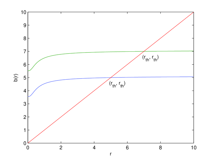
Figure 1: The shape function.

Eq. (7) is valid for any $r_{th}$, the wormhole can be macroscopic. We also observe that $b(r)<r$ for $r>r_{th}$.

Since we are interested in the detection of wormholes in the outer regions of the halo, we need to recall that in this region test particles move in circular orbits. So it is assumed that $e^{2\Phi(r)}$ in line element (1) is given by

$$e^{2\Phi(r)}=\left(\frac{r}{b_{0}}\right)^{l}.$$ (8)

Here $l=2(v^{\phi})^{2}$, where $v^{\phi}$ is the tangential velocity and $b_{0}$ an integration constant [12]. According to Ref. [13], $l=0.000001$. In a wormhole setting, we can assume that the center of the wormhole also serves as the origin of $\rho(r)$. So the line element becomes

$$ds^{2}=-\left(\frac{r}{b_{0}}\right)^{l}dt^{2}+\frac{dr^{2}}{1-b(r)/r}+r^{2}(d\theta^{2}+\text{sin}^{2}\theta\,d\phi^{2}).$$ (9)

3 Gravitational lensing

Interest in strong gravitational lensing has increased over time in large part due to a series of studies by Virbhadra et al. [14, 15, 16, 17]. In particular, gravitational lensing has been studied from the strong-field perspective by means of the analytic method developed by Bozza [18] to calculate the deflection angle. This method was used in Refs. [19, 20] to study two special models by Lemos et al. [21], one of which is the Ellis wormhole.

To apply these methods to the wormholes in this paper, we will follow the procedures in Refs. [19, 20]. To do so, we will take the line element to be

$$ds^{2}=-A(x)dt^{2}+B(x)dx^{2}+C(x)(d\theta^{2}+\sin^{2}\theta\,d\phi^{2}),$$ (10)

where $x$ is the radial distance in Schwarzschild units, i.e., $x=r/2M$. Then

$$x_{0}=\frac{r_{0}}{2M}$$ (11)

denotes the closest approach to the light ray. Thus from Eq. (7),

$$\frac{1}{2M}b(r)=\frac{4M}{\pi(2M)}\left(\text{tan}^{-1}\frac{r/2M}{\sqrt{\theta}/2M}-\frac{(r/2M)(\sqrt{\theta}/2M)}{(r^{2}+\theta)/(2M)^{2}}\right.\\ \left.-\text{tan}^{-1}\frac{r_{th}/2M}{\sqrt{\theta}/2M}+\frac{(r_{th}/2M)(\sqrt{\theta}/2M)}{(r_{th}^{2}+\theta)/(2M)^{2}}\right)+\frac{r_{th}}{2M}.$$ (12)

In the discussion below, we let $\sqrt{\beta}=\sqrt{\theta}/2M$.

Now using the lens equation in Ref. [15], it is shown in Refs. [19, 20] that the deflection angle $\alpha(x_{0})$ consists of the sum of two terms:

$$\alpha(x_{0})=\alpha_{e}+I(x_{0}).$$ (13)

Here

$$\alpha_{e}=-2\,\text{ln}\left(\frac{2a}{3}-1\right)-0.8056$$ (14)

is due to the external Schwarzschild metric outside the wormhole’s mouth $r=a$; $I(x_{0})$ is the contribution from the internal metric, first derived in Ref. [14]:

$$I(x_{0})=2\int^{\infty}_{x_{0}}\frac{\sqrt{B(x)}\,dx}{\sqrt{C(x)}\sqrt{\frac{C(x)A(x_{0})}{C(x_{0})A(x)}-1}}.$$ (15)

From our line element (9) and the shape function (12) [with $\beta=\theta/(2M)^{2}$], we obtain

$$I(x_{0})=\\ \int^{a}_{x_{0}}R(x)\,dx,$$ (16)

where

$$R(x)=\\ \frac{2}{\sqrt{x^{2}\left\{1-\frac{1}{x}\left[\frac{2}{\pi}\left(\text{tan}^{-1}\frac{x}{\sqrt{\beta}}-\frac{x\sqrt{\beta}}{x^{2}+\beta}-\text{tan}^{-1}\frac{x_{th}}{\sqrt{\beta}}+\frac{x_{th}\sqrt{\beta}}{x_{th}^{2}+\beta}\right)+x_{th}\right]\right\}}\sqrt{\frac{x^{2-l}}{x_{0}^{2-l}}-1}}.$$ (17)

To see where this integral diverges, we make the change of variable $y=x/x_{0}$, so that $x=x_{0}y$ and $x_{th}=x_{0}y_{th}$:

$$I(x_{0})=\int_{1}^{a/x_{0}}S(y)\,dy,$$ (18)

where

$$S(y)=\\ \frac{2}{\sqrt{(y^{4-l}-y^{2})\left\{1-\frac{1}{x_{0}y}\left[\frac{2}{\pi}\left(\text{tan}^{-1}\frac{x_{0}y}{\sqrt{\beta}}-\frac{x_{0}y\sqrt{\beta}}{x_{0}^{2}y^{2}+\beta}-\text{tan}^{-1}\frac{x_{0}y_{th}}{\sqrt{\beta}}+\frac{x_{0}y_{th}\sqrt{\beta}}{x_{0}^{2}y_{th}^{2}+\beta}\right)+x_{0}y_{th}\right]\right\}}}.$$ (19)

The radicand $F(y)$ in the denominator can be expanded in a Taylor series around $y=1$. Letting

$$g(y)=1-\frac{1}{x_{0}y}\left[\frac{2}{\pi}\left(\text{tan}^{-1}\frac{x_{0}y}{\sqrt{\beta}}-\frac{x_{0}y\sqrt{\beta}}{x_{0}^{2}y^{2}+\beta}-\text{tan}^{-1}\frac{x_{0}y_{th}}{\sqrt{\beta}}+\frac{x_{0}y_{th}\sqrt{\beta}}{x_{0}^{2}y_{th}^{2}+\beta}\right)+x_{0}y_{th}\right],$$ (20)

we obtain

$$F(y)=(2-l)g(1)(y-1)\\ +\left[\frac{1}{2}(5-l)(2-l)g(1)+(2-l)g^{\prime}(1)\right](y-1)^{2}\\ +\text{higher powers}.$$ (21)

As discussed in Ref. [22], if $g(1)\neq 0$, the integral converges due to the leading term $(y-1)^{1/2}$ resulting from the integration. If $g(1)=0$, then the second term leads to $\text{ln}\,(y-1)$, and the integral diverges.

Next, suppose in Eq. (7), we choose $r_{th}=r_{0}$, the nearest approach, for the radius of the throat. Since $x_{th}=r_{th}/2M$ and $y_{th}=x_{th}/x_{0}$, we now have $y_{th}=1$. Then

$$g(y)=1-\frac{1}{x_{0}y}\left[\frac{2}{\pi}\left(\text{tan}^{-1}\frac{x_{0}y}{\sqrt{\beta}}-\frac{x_{0}y\sqrt{\beta}}{x_{0}^{2}y^{2}+\beta}-\text{tan}^{-1}\frac{x_{0}}{\sqrt{\beta}}+\frac{x_{0}\sqrt{\beta}}{x_{0}^{2}+\beta}\right)+x_{0}\right].$$ (22)

As a result, $g(1)=0$ and the above integral diverges. According to Refs. [19, 20], we have a photon sphere at the throat $r=r_{th}$. Such a photon sphere can, in principle, be detected.

4 Comparison to the NFW model

It is shown in Ref. [22] that the Navarro-Frenk-White (NFW) model predicts a throat size of 0.40 ly. So if a wormhole has a throat size that is significantly different from 0.40 ly, it cannot be due to the dark matter model, but it would be consistent with a noncommutative-geometry background.

An obvious competitor for the dark-matter model is $f(R)$ modified gravity. Let us therefore consider the gravitational field equations (for the special case $\Phi^{\prime}\equiv 0$) proposed by Lobo and Oliveira [23]:

$$\rho(r)=F(r)\frac{b^{\prime}(r)}{r^{2}},$$

$$p_{r}(r)=-F(r)\frac{b(r)}{r^{3}}+F^{\prime}(r)\frac{rb^{\prime}(r)-b(r)}{2r^{2}}-F^{\prime\prime}(r)\left[1-\frac{b(r)}{r}\right],$$

$$p_{t}(r)=-\frac{F^{\prime}(r)}{r}\left[1-\frac{b(r)}{r}\right]+\frac{F(r)}{2r^{3}}[b(r)-rb^{\prime}(r)],$$

where $F=\frac{df}{dR}$. The curvature scalar is given by

$$R(r)=\frac{2b^{\prime}(r)}{r^{2}}.$$

Using these equations, it is shown in Ref. [24] that to account for dark matter, it is sufficient for $F$ to be close to unity and $F^{\prime}$ to be close to zero. So if $\rho(r)$ is taken from the NFW model, the results are likely to be similar. This suggests that a significant departure from a radius of 0.40 ly can be taken as evidence for a noncummutative-geometry background.

5 Summary

The first part of this paper confirms that a noncommutative-geometry background with a static and spherically symmetric gravitational source having the form

$$\rho(r)=\frac{M\sqrt{\theta}}{\pi^{2}(r^{2}+\theta)^{2}}$$

can support traversable wormholes. Such wormholes may be located in the outer regions of the galactic halo. Using a method for calculating the deflection angle proposed by Bozza [18], it is shown that the deflection angle diverges at the throat, thereby producing a detectable photon sphere. By allowing a comparison to other models, such as the NFW model and $f(R)$ modified gravity, the procedure is likely to favor a model based on noncommutative geometry.

References

- [1] M.S. Morris and K.S. Thorne, “Wormholes in spacetime and their use for interstellar travel: A tool for teaching general relativity,” Amer. J. Phys. 56, 395 (1988).
- [2] E. Witten, “Bound states of strings and -branes,” Nucl. Phys. B 460, 335 (1996).
- [3] N. Seiberg and E. Witten, “String theory and noncommutative geometry,” JHEP 9909, 032 (1999).
- [4] A. Smailagic and E. Spalluci, “Feynman path integral on the non-commutative plane,” J. Phys. A 36, L-467 (2003).
- [5] A. Smailagic and E. Spalluci, “UV divergence-free QFT on noncommutative plane,” J. Phys. A 36, L-517 (2003).
- [6] P. Nicollini, A. Smailagic, and E. Spalluci, “Noncommutaative geometry inspired Schwarzschild black hole,” Phys. Lett. B 632, 547 (2006).
- [7] P.K.F. Kuhfittig, “Macroscopic wormholes in noncommutative geometry,” Int. J. Pure Appl. Math. 89, 401 (2013).
- [8] J. Liang and B. Liu, “Thermodynamics of noncommutative geometry inspired BTZ black holes based on Lorentzian smeared mass distribution,” EPL 100, 30001 (2012).
- [9] K. Nozari and S.H. Mehdipour, “Hawking radiation as quantum tunneling for a noncommutative Schwarzschild black hole,” Class. Quant. Grav. 25, 175015 (2008).
- [10] P.K.F. Kuhfittig and V. Gladney, “Revisiting galactic rotation curves given a noncommutative-geometry background,” J. Mod. Phys. 5, 1931 (2014).
- [11] P.K.F. Kuhfittig, “Macroscopic traversable wormholes with zero tidal forces inspired by noncommutative geometry,” Int. J. Mod. Phys. D 24, 1550023 (2015).
- [12] K.K. Nandi, I. Valitov, and N.G. Migranov, “Remarks on a spherical field halo in galaxies,” Phys. Rev. D 80, 047301, (2009).
- [13] K.K. Nandi, A.I. Filippov, F. Rahaman, S. Ray, A.A. Usmani, M. Kalam, and A. DeBenedictis, “Features of galactic halo in a brane world model and observational constraints,” Mon. Not. Roy. Astron. Soc. 399, 2079 (2009).
- [14] K.S. Virbhadra, D. Narasimha, and S.M. Chitre, “Role of the scalar field in gravitational lensing,” Astron. Astrophys. 337, 1 (1998).
- [15] K.S. Virbhadra and G.F.R. Ellis, “Schwarzschild black hole lensing,” Phys. Rev. D 62, 084003 (2000).
- [16] C.-M. Claudel, K.S. Virbhadra, and G.F.R. Ellis, “The geometry of photon surfaces,” J. Math. Phys. 42, 818 (2001).
- [17] K.S. Virbhadra, “Relativistic images of Schwarzschild black hole lensing,” Phys. Rev. D 79, 083004 (2009).
- [18] V. Bozza, “Gravitational lensing in the strong field limit,” Phys. Rev. D 66, 103001 (2002).
- [19] J.M. Tejeiro and E.A. Larranaga, “Gravitational lensing in asymptotically flat wormholes,” arXiv: gr-qc/0505054.
- [20] J.M. Tejeiro and E.A. Larranaga, “Gravitational lensing by wormholes,” Rom. J. Phys. 57, 736 (2012).
- [21] J.P.S. Lemos, F.S.N. Lobo, and S. Quinet de Oliveira, “Morris-Thorne wormholes with a cosmological constant,” Phys. Rev. D 68, 064004 (2003).
- [22] P.K.F. Kuhfittig, “Gravitational lensing of wormholes in the galactic halo region,” Eur. Phys. J. C 74, 2818 (2014).
- [23] F.S.N. Lobo and M.A. Oliveira, “Wormhole geometries in modified theories of gravity,” Phys. Rev. D 80, 104012 (2012).
- [24] P.K.F. Kuhfittig, “A simple argument for dark matter as an effect of slightly modified gravity,” Adv. Studies Theor. Phys. 8, 349 (2014).