Molecular Scale Hydrophobicity in Varying Degree of Planar Hydrophobic Nanoconfinement

Abstract

We have studied the molecular scale hydrophobicity of an apolar solute, argon, confined between hydrophobic planar surfaces with different confinement widths. Specifically, we find that the hydrophobicity exhibits a non-monotonic behavior with confinement width. While hydrophobicity is usually large compared to bulk value, we find a narrow range of confinement width where the hydrophobicity displays similar values as in bulk water. Furthermore, we develop a simple model taking into account the entropic changes in nanoconfined geometry, which enables us to calculate potential of mean force between solutes as the conditions change from bulk to different degrees of planar nanoconfinement. Our results are important in understanding nanoconfinement induced stability of apolar polymers, solubility of gases, and may help design better systems for Enhanced Oil Recovery.

I Introduction

Confined systems are prevalent in nature. Examples of confinements include intracellular water and biomolecules to gases and liquids trapped in porous rock sediments Tang2006 ; Hartls2011 ; Wu2013 . One can expect that when confinement length scales approach the inherent characteristic molecular length scales, such as various correlation lengths, the properties of a system may deviate from bulk Kumar2005 .

It is widely believed that besides the interaction of solvent with solutes, thermodynamic states and dynamics of solvent, water in case of aqueous systems, are important in dictating the behavior of solubility of solutes. Nanoconfinement induced changes in the properties of water is quite extensively studied in recent times Koga2000 ; Koga2001 ; Truskett2001 ; Zangi2003 ; Gallo07 ; Johnston2010 ; Han2010 ; Chen2006 ; Liu04 ; Nicolas2007 ; Nicolas2009 ; Mallamace2011 . It has been shown that when water is confined to length scales of few molecular diameters, water exhibit distinct structural and dynamical changes as compared to bulk water Raviv2001 . Koga et. al. have studied liquid-solid phase transitions in water confined between hydrophobic surfaces and have shown that for appropriate dimensions of the flat hydrophobic confinements, water can undergo a first-order phase transition from a bilayer liquid to a bilayer hexagonal ice Koga2000 ; Koga2001 . Further studies of water in nanoconfinements have suggested a range of exotic structural phases such as n-fold crystal (n=2,4,6, and 12) in bilayer water Johnston2010 . Bai et. al. have found a variety of polymorphic and polyamorphic transitions in bilayer water confined between hydrophobic surfaces Bai2012 . Recently, Han et. al. have studied liquid-solid phase transitions in bilayer water confined between planar hydrophobic surfaces Han2010 . They find that nature of liquid-solid phase transition changes from a first-order transition at low densities to a continuous liquid-solid transition at high densities. Besides the structural changes in nanoconfinement, it has been shown that the physical property such as temperature of maximum density (TMD) of water shifts to lower temperature and lower density in the temperature-density plane as compared to bulk water Kumar2005 . Gallo et. al. have studied the effect of nanoconfinement on the dynamics and thermodynamics of water and found that the water confined in nanopores exhibits different dynamical regimes depending on the distance of water from the surface Gallo07 . The effects of morphology and charges of confining surfaces have been explored in Ref. Varma2010 ; Nicolas2007 .

Aqueous solubility and hydrophobicity of solutes is an active area of research due to its implication in a large variety of physical phenomena including protein stability and folding Wiggins1997 ; Chandler1999 ; Asbaugh2002 ; Dill2005 ; Garde2006 ; Buldyrev07 ; Zhou2002 , hydrate formation Walsh2009 , and enhanced oil recovery Wu2013 . Studies of solubility of hydrocarbon solutes in water suggests that they exhibit anomalous solubility in water Battino1982 ; Battino1986 ; Battino1987 . For example methane solubility in water shows a minimum around $320$ K and increases on both sides of this temperature. Low temperature increase of solubility of apolar solutes is implicated in cold unfolding of proteins and apolar polymers Buldyrev07 . In more recent works, Mallamace et. al. have explored the influence of water on protein properties including protein folding and dynamic transition in proteins at low temperatures Mallamace2011 ; Mallamace2014 . Recent computational studies have investigated the effect of nanoconfinement on the phase behavior of oil-water mixture in an effort to improve the existing enhanced oil recovery technologies Wu2013 . Studies of solubility and ordered phase formation of gases in solid ice phases have attracted wide attention due to its importance in hydrocarbon processing and sustainable energy production Sloan2008 ; Sloan2003 ; Walsh2009 ; Debenedetti2009 .

Although a large body of literature exists on the solubility and hydrophobicity of apolar solutes in bulk water, the effect of nanoconfinement on the solubility and hydrophobicity remains poorly understood. Since both thermodynamic and dynamic properties of water may vary in nanoconfinement, one may expect that the hydrophobicity may also be different from the bulk . Water in biological systems is under the conditions which differ greatly from the bulk hence the bulk behavior of water may not be relevant under those conditions. Therefore, a good understanding of the behavior of hydrophobicity of any molecule would only be possible if a detailed study of the these conditions are explored.

In this article, we study molecular scale hydrophobicity of an apolar solute, argon, in planar hydrophobic nanoconfinement of varying length scales. In Method section, we describe the simulation methods, in Results section, we discuss the results and finally we conclude with Summary and Discussion section.

II System and Method

We performed molecular dynamics simulations to calculate potential of mean force (PMF) McQuarrie between argon atoms dissolved in TIP3P (transferable interaction potential three points) JorgensenXX ; jorgensen2 water-like solvent confined between two structured planar hydrophobic surfaces separated by a distance $L_{\rm z}$. The atoms on the surfaces were arranged in a hexagonal closed packing with a distance $\sigma_{S}=0.339$ nm and they do not interact with each other. The positions of the surface atoms were restrained to their respective mean positions by a harmonic potential with a force constant $10^{4}$ kJ/mol. In order to mimic hydrophobic surfaces, carbon atoms were chosen to be surface atoms. The interaction between the surface atoms and the oxygen of the water molecule is modeled using $6-12$ Lennard-Jones (LJ) potential $U(r)$

$$U(r)=4\epsilon[(\frac{\sigma}{r_{SO}})^{12}-(\frac{\sigma}{r_{SO}})^{6}]$$ (1)

where $r_{SO}$ is the distance between the surface atom and oxygen of water molecule, and $\sigma=(\sigma_{\rm S}+\sigma_{\rm OW})/2$ and $\epsilon=\sqrt{\epsilon_{\rm S}\epsilon_{\rm OW}}$. $\sigma_{\rm OW}$ and $\epsilon_{\rm OW}$ are the parameters of the Lennard-Jones interaction between oxygen atoms of water molecules JorgensenXX ; jorgensen2 .

We performed simulations of confined water and solutes between hydrophobic surfaces in NVT-ensemble with effective density of the system, $\rho=1.00$ g/cm³. The effective density of the system is obtained by calculating the effective confinement width available for water molecules for a given center-to-center distance, $L_{\rm z}$, between the surface atoms. The effective confinement width, $\xi$, available to water molecules is calculated as

$$\xi=Lz-\frac{(\sigma_{\rm OW}+\sigma_{SO})}{2}$$ (2)

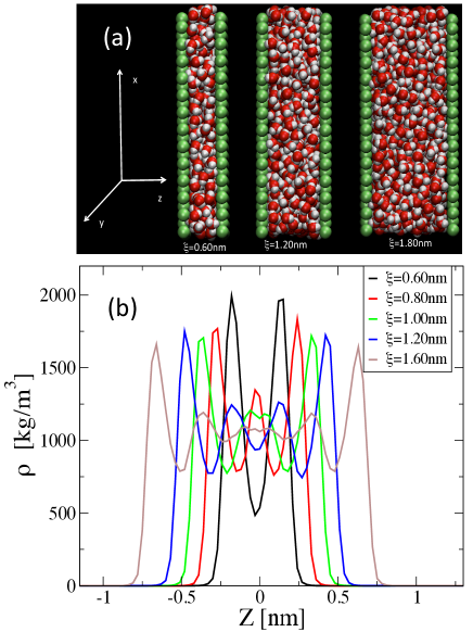
Figure 1: (color online) (a) Schematic of nonoconfined system. (b) Potential of mean force (PMF) between two argon atoms as a function of distance $r$ between argon atoms for different confinement width $\xi$.

The equations of motion were integrated with a time step of $0.001$ ps and velocity rescaling was used to attain constant temperature and Berendsen barostat for constant pressure in Gromacs 4.5 Gromacs . Periodic boundary conditions were applied in XY-directions. We use constrained molecular dynamics method for the calculation of PMF for seven different effective confinement widths $\xi=0.6,0.8,1.0,1.2,1.4,1.6$, and $1.8$ nm. Images of some of the representative configurations studied here are shown in Fig. 1(a).

After the system was equilibrated for $1$ ns at $T=300$ K for respective confinements, we constrain the argon atoms at fixed values of distances with a harmonic potential with a spring constant $k_{c}=1000$ kJ/mol. After the equilibration step, we ran the simulations for additional $1$ ns for each constraining distances $d$ between $0.26$ and $1.0$ nm at an interval of $0.02$ nm. Potential of mean force was corrected for volume entropy at T$=300$ K. For the range of confinement widths studied here, we find strong layering of water near the surfaces as suggested by the transverse density profile of water along the confinement direction $z$ (see Figure 1(b)).

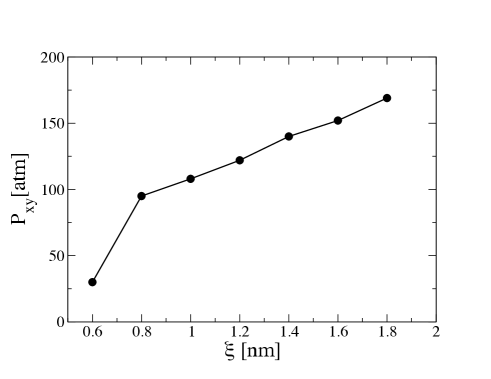
Figure 2: Lateral pressure $P_{\rm xy}$ as a function of effective confinement width $\xi$ for the fixed density $\rho={\rm 1.0g/cm^{3}}$. $P_{\rm xy}$ decreases monotonically with confinement width.

While the effective density of the system remains the same, the lateral pressure along the periodic directions, $P_{\rm xy}$, varies for different confinement widths as shown in Fig. 2. $P_{\rm xy}$ monotonically increases with effective confinement width $\xi$.

III Results

Potential of mean force and second Virial coefficient

To quantify hydrophobicity, we first calculate PMF, $w(r)$, for different confinement widths using umbrella sampling Eerden1989 . To use umbrella sampling, the distance between the argon atoms is chosen as the reaction co-ordinate. Within this scheme, a constraining potential is added to the Hamiltonian. The modified Hamiltonian of the system with the constraining potential with a perturbation parameter $\lambda$ can be written as

$$H(\lambda)=H_{0}+\frac{1}{2}k_{c}(r-r_{0}(\lambda))^{2}$$ (3)

where $k_{c}$ is the spring constant of the constraining potential and $r_{0}$ is the constraining distance. The free energy change $\Delta G$ between two arbitrary points along the reaction coordinate is given by

$$\Delta G=\int{(\frac{\partial G}{\partial\lambda})_{\lambda}d\lambda}=\int{(\frac{\partial H}{\partial\lambda})_{\lambda}d\lambda}=\int{-\left<k_{c}(r-r_{0})\right>_{r_{0}}dr_{0}}$$ (4)

Hence the free energy difference between two states along the reaction coordinate is integral of the mean force between the state points. The PMF, $w(r)$, for a given state point along the reaction coordinate with respect to a reference state is

$$w(r)=-\int_{r_{\rm ref}}^{r}{<F(r_{0}^{\prime})>dr_{0}^{\prime}}+2k_{B}T{\rm ln}(r)+C.$$ (5)

where, $<F(r_{0}^{\prime})>$ is the mean force for a given constraining distance $r_{0}^{\prime}$, $r_{\rm ref}$ is the position along the reaction coordinate for the reference state, and the second term in the above expression is the volume entropy correction. We choose the reference state to be $r_{\rm ref}=1$ nm where $w(r_{\rm ref})=0$.

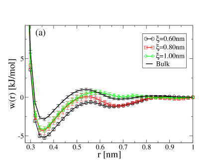
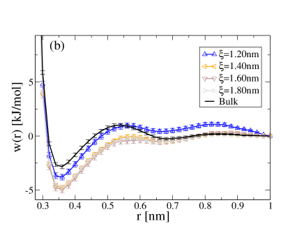
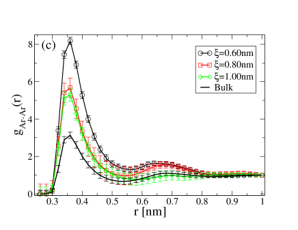
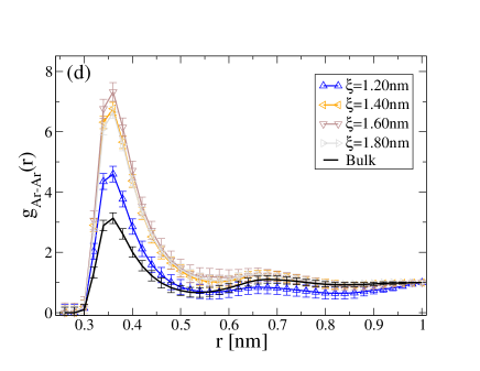
Figure 3: (color online) Potential of mean force between argon in nanoconfiment for different confinement widths (a) $\xi=0.6,0.8,1.0$, and (b) $\xi=1.2,1.4,1.6,1.8$ nm respectively. For a comparision, we also show PMF for argon in bulk water at $T=300$ K and $P=1$ atm. Argon-argon radial distribution function $g_{\rm Ar-Ar}(r)$ calcuated using PMF $w(r)$ for confinement widths (c) $\xi=0.6,0.8,1.0$ nm, and (d) $\xi=1.2,1.4,1.6,1.8$ nm.

In Fig. 3(a) and (b), we show PMF, $w(r)$, as a function of distance $r$ between argon atoms for all the confinement widths. For a comparison, we also show the PMF for argons in bulk water at $P=1$ atm and $T=300$ K. $w(r)$ for bulk system exhibits two prominent minima, one at $r\approx 0.35$ nm and another at $r\approx 0.68$ nm respectively. While the position of the first minimum of $w(r)$ remains unchanged in confinement, the position of the second minimum decreased to $r\approx 0.64$ nm for the smallest $\xi$. Moreover, while the first minimum becomes deeper monotonically with decreasing confinement width, the second minimum shows a non-monotonic behavior with $\xi$ suggesting a non-trivial solvation structure dependence with confinement width $\xi$.

In Fig. 3(c) and (d), we show the radial distribution function between argons as calculated from $g_{\rm Ar-Ar}(r)=e^{-\beta w(r)}$ for all the confinement widths studied here. It is clear that solvation structure of argons in water in nanoconfinement exhibits a non-trivial dependence on the confinement width of confining surfaces. Since, this non-trivial behavior of PMF or $g_{Ar-Ar}(r)$ for the second shell makes it harder to interpret the hydrophobicity directly by looking at them, therefore to quantify hydrophobicity, we next calculate the second Virial coefficient.

The second Virial coefficient $B_{2}$ for a mono-component system is given by

$$B_{2}=-\frac{1}{2}\int_{0}^{\infty}(e^{-\beta w(r)}-1)d\Gamma$$ (6)

where $\beta=\frac{1}{k_{B}T}$, and $d\Gamma$ is the volume element corresponding to the separation $r$. $w(r)$ is related to the solute-solute pair correlation function $h(r)$ as

$$w(r)=-k_{B}T\ln[h(r)+1]$$ (7)

and hence

$$B_{2}=-\frac{1}{2}\int h(r)d\Gamma$$ (8)

A positive value of $B_{2}$ indicates an effective repulsive interaction between the solutes and hence larger solubility and a negative value suggest an effective attractive interaction and hence smaller solubility. The volume element, $d\Gamma=A(r,\xi)dr$, in the planar confinement depends on both $r$ and $\xi$ and can be derived by first deriving the average surface area $A(r,\xi)$ corresponding to solute separation $r$. Let’s assume that the surfaces are represented by two planes; one at $z=0$ and another at $z=\xi$. Assuming that the first particle can assume any value of $z$ between $0$ and $\xi$, we can next write the average area, $A(r;\xi)$, traversed by the radial vector joining two particles as (a detailed derivation of $A(r;\xi)$ is given in the Supplementary Information):

$$A^{*}(r;\xi)=\left\{\begin{array}[]{rl}4\pi r^{2}[1-\frac{r}{2\xi}]&\mbox{ if $r\leq\xi/2$}\\ 2\pi r\xi(1-(\frac{r}{\xi})^{2})+4\pi r^{2}(1-\frac{\xi}{2r})&\mbox{ if $\xi/2\leq r\leq\xi$}\\ 2\pi r\xi&\mbox{ if $r\geq\xi$}\end{array}\right.$$ (9)

The above expression suggests that the accessible area to arrange a pair of particle of fixed separation $r$ decreases with $r$ as compared to bulk.

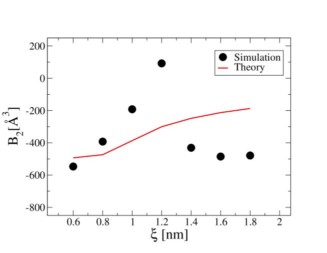
Figure 4: (color online) Second Virial coefficient $B_{2}$ between argons as a function confinement width $\xi$. Also shown is the curve obtained using entropic consideration in confinement (see Section V).

In Fig. 4, we show the second Virial coefficient $B_{2}$ as a function of $\xi$. The values of $B_{2}$ are significantly smaller compared to the bulk value of $B_{2}$ ($-17\AA^{3}$) at $P=1$ atm and $T=300$ K except for $\xi=1.2$ nm, suggesting that the hydrophobicity of argon increases in nanoconfinement. Moreover, $B_{2}$ exhibits a nonmonotonic dependence on $\xi$. $B_{2}$ first increases with increasing $\xi$ for $\xi=0.6-1.2$ nm and then it falls off sharply with a weak dependence on $\xi$ for $\xi=1.4-1.80$ nm.

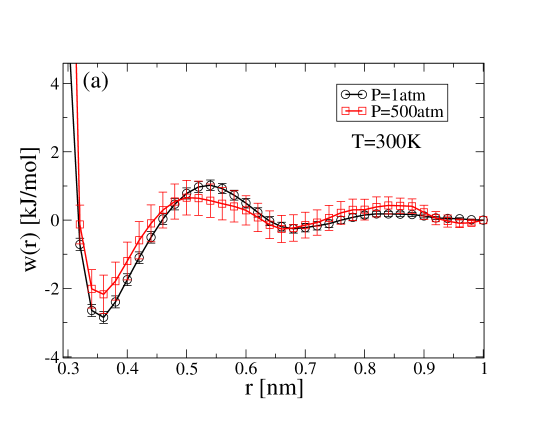
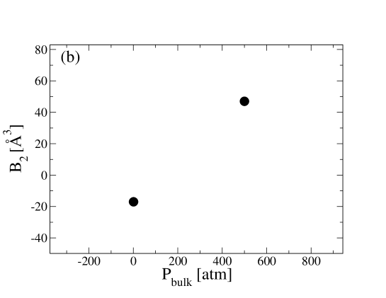
Figure 5: (color online) (a) Potential of mean force between argon, $w(r)$, for bulk system for two different pressures $P=1,$ and $500$ atm and temperature $T=300$ K. (b) Second Virial coefficient $B_{2}$ for two pressures $P=1,$ and $500$ atm and temperature $T=300$ K.

Since the simulations are done in NVT-ensemble, the pressure for different values of $\xi$ are different even when the effective density remains the same. One may argue that the change in hydrophobicity is just due to pressure increase as the confinement width decreases. To test this we next calculated vlaues of $B_{2}$ for argon for two different pressures $P=1$ and $500$ atm in bulk water. The pressures were chosen such that they cover the pressure ranges for the nanoconfined system. In Fig. 5 (a), we show the PMF for P=1 and 500 atm for the bulk system at $T=300$ K. The second Virial coefficient $B_{2}$ for $P=1,500$ atm are $-17$ and $53$ $A^{o^{3}}$ respectively. We find that the bulk values of $B_{2}$ differ greatly from the nanoconfined values except for $\xi=1.2$ nm, for which the system shows a comparable value of $B_{2}$. To this end, it clear that the magnitude of hydrophobicity in nanoconfinement is drastically different from the bulk. Moreover, our results indicate subtle changes in solvation and effective hydrophobicity upon nanoconfinement. Indeed, small changes in the length scale of nanoconfining regions may lead to large changes in hydrophobicity.

From bulk PMF to confined PMF

Nanoconfinement results in changes in arranging a solute particle around a reference particle (see Supplementary Information) –namely a decrease in the volumetric arrangement, we can define the change in entropy $\Delta S_{1}(r;\xi)$ in nanoconfinement over a bulk system as:

$$\Delta S_{1}(r;\xi)=\left\{\begin{array}[]{rl}k_{B}\ln(1-\frac{r}{2\xi})&\mbox{ if $0\leq r\leq\xi/2$}\\ k_{B}\ln[(1-\frac{\xi}{2r})+\frac{\xi}{2r}(1-(\frac{r}{\xi})^{2})]&\mbox{ if $\xi/2\leq r\leq\xi$}\\ k_{B}\ln(\frac{\xi}{2r})&\mbox{ if $\xi\leq r\leq r_{0}$}\end{array}\right.$$ (10)

where $r_{0}$ is the separation between solutes such that ${\rm lim}_{r->r_{0}}w(r)=0$. Note that $r_{0}$ is the distance beyond which the system loses two-point correlations. In our case, we assume $r_{0}=1$ $nm$. The validity of above expression ranges for the values of $r$ over which the solute particles are correlated beyond which the two point entropy would be zero for both bulk and confined system. Since the entropy decreases as $r$ is increased, we argue that the system with solute nanoconfinement will try to increase the configurations pertaining to larger entropy in order to minimize free energy. Hence, we can assume an additional thermodynamic driving potential $-T\Delta S_{1}(r;\xi)$ acting on a pair of particles. This entropic penalty will make small distances between solutes more favorable as they correspond to higher entropy. Taking this into account, we can write the modified PMF in nanoconfinement $w^{*}(r;\xi)$ as

$$w^{*}(r;\xi)=w_{\rm bulk}(r)-T\Delta S_{1}(r)$$ (11)

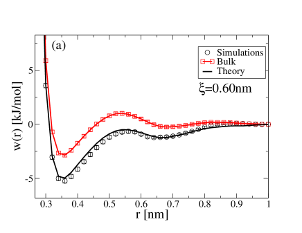
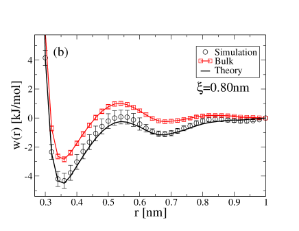
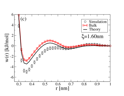
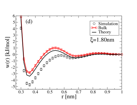
Figure 7: (color online) Comparision of potential of mean force calculated from simulation with theory for confinement widths (a) $\xi=0.60$ nm, (b) $\xi=0.80$ nm, (c) $\xi=1.60$ nm, and (d) $\xi=1.80$ nm. While the PMF predicted from theory does reasonably well for smaller $\xi$, it deviates from the PMF calculated from simulations for larger $\xi$.

The $w^{*}(r;\xi)$ is then normalized such that $w^{*}(r=1nm;\xi)=0$. In Fig. 7, we compare PMF computated from simulations and PMF from Eq. 11 for confinement widths $\xi=0.60$ nm, $\xi=0.80$ nm, $\xi=1.60$ nm, and, $\xi=1.80$ nm. We find that the PMF predicted by theory does reasonably well for smaller $\xi$ but it deviates from the PMF calculated from simulations for larger $\xi$. The deviation of theory could presumably results from absence of enthalpic consideration. We show the values of $B_{2}$ calculated from $w^{*}(r;\xi)$ for different values of confinement widths in Fig. 4 along with the computed values of $B_{2}$ from simulations.

We find that simple argument of entropy decrease of configurations with different separation of a pair of solute atoms in confinement works well with planar geometry studied here. Indeed, a similar argument can be made for different geometries of confinement such as cylindrical nanoconfinement.

Solvation Structure

Next, we investigate the solvation structure in order to find a clue to the anomalous hydrophobicity behavior for $\xi=1.2$ nm by investigating the radial distribution of water and argon. For water, we calcualte the oxygen-oxygen lateral radial distribution function, $g_{\rm oo}(r_{xy})$ as a function their lateral distance $r_{\rm xy}$. In Fig. 8 (a), we show $g_{\rm oo}(r_{\rm xy})$ for all the confinement widths $\xi$. We find that, water tends to order laterally with the decrease of confinement width as suggested by increased first and second peaks in $g_{\rm oo}(r_{\rm xy})$ upon decrease of $\xi$. In Fig. 8(b), we show the radial distribution function between oxygen of water and argon, $g_{O-Ar}(r)$ calculated from long simulations of water-argon system ($4$ ns for each confinement width). While the structure of the first solvation shell ($r\approx 0.36$ nm) does not show any appreciable change with $\xi$ except the decreasing value of the first peak, the second shell becomes much wider and the corresponding peak moves to slightly larger values of $r$. Combining the results on PMF between argon and solvation structure, it seems that non-monotonic dependence of second shell on $\xi$ may explain the increased value of $B_{2}$ for $\xi=1.2$ nm and will require further investigation.

IV Summary and Discussion

We have studied molecular scale hydrophobicity of a small apolar solute in nanoconfinement by calculating the second Virial coefficients from the potential of mean force between apolar solutes in water confined between hydrophobic surfaces with different confinement widths. We find that: (i) hydrophobicity of apolar solutes usually increases as the confinement width decreases at constant transverse pressure, (ii) hydrophobicity exhibits an anomalous region, where the hydrophobicity becomes similar to the values in bulk water. Furthermore, we find that this anomalous region of confinement widths correspond to changes in second and third solvation shell. We develop a simple entropic theory to find effective potential of mean force in nanoconfinement. The predicted PMF from theory works reasonably well for smaller confinement widths and allows to predict the effective hydrophobicity in nanoconfinement when the potential of mean force in bulk is known.

Hydrophobicity plays important roles in many physical systems including the folding of polypeptides. We hypothesize that large changes in hydrophobicity with very small changes in length scale of nanoconfining regions could be very important in maintaining the rate of folding in biological systems such as chaperone proteins in a chemically non-specific way. A very good example of this is GroEL-GroES complex in bacteria, which is induced upon temperature shocks cage . To counteract the increase of temperature and hence unfolding of polypeptides, nature has evolved a complex machinery. An unfolded polypeptide is directed into a chaperon complex such as GroEL-GroES and stays inside the cage formed by the protein complex where it folds much faster than it would in the bulk region cage . We argue based on our results that when and unfolded or partially folded polypeptide enters this complex, a large part of the folding may occur in the neck-region before it reaches the cage. Moreover, we hypothesize that the modulating diameter of this chaperon complex would naturally be helpful in modulating the rate of folding in a chemically non-specific way.

In summary, our results are important in understanding nanoconfinement induced stability of apolar polymers, solubility of gases and may help design better systems for enhanced oil recovery. While our work has explored the planar hydrophobic confinement in details, the geometry and charge distribution of the confining surfaces may affect the hydrophobicity. Furthermore, effect of solute size consideration is also a determining factor for hydrophobicity which we will explore in future work.

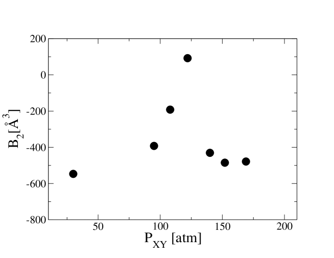
Figure 6: Second Virial coefficient $B_{2}$ as a function of lateral pressure $P_{\rm xy}$.

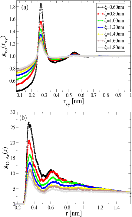
Figure 8: (a) Lateral oxygen-oxygen radial distribution function, $g_{\rm oo}(r_{\rm xy})$ of water for various confinement width. (b) Oxygen-Argon radial distribution function, $g_{\rm O-Ar}(r)$, for all the confinement widths studied here.

Supplementary Information:

Effective surface area traced by a particle at a distance $r$ from another particle

Let’s assume that two infinite planar surfaces are located at $z=0$ and $z=\xi$ respectively. We are interested in the average surface area traced by a particle at a fixed distance $r$ from the reference particle. It is easy to see that the average surface area for a fixed $r$ depends on both $r$ and $\xi$. When the reference particle is closer to the surface the area is smaller compared to when the reference particle is sitting close to the center of the surfaces.

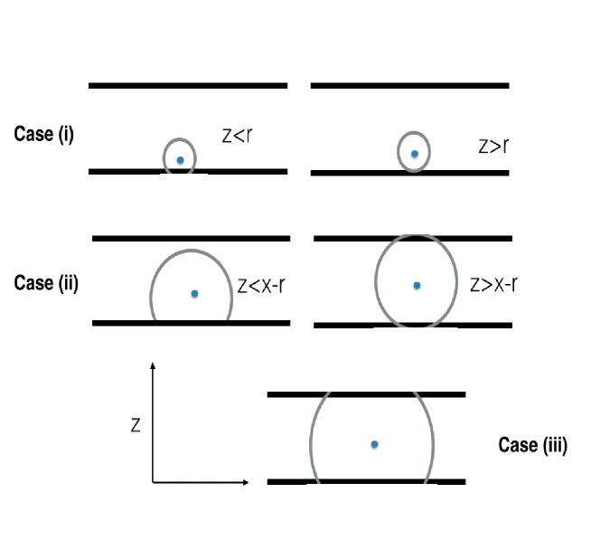
Figure S1: Schematics of the regions of $r$ discussed above for a confinement width $\xi$.

Three different regimes of $r$ – (i) $0\leq r\leq\xi/2$, (ii) $\xi/2\leq r\leq\xi$, and (iii) $r\geq\xi$ can be noted. Furthermore, from the symmetry of the system, it is sufficient to calculate the average area traced by the second particle for different positions of the reference particle only along the $z$ direction. Let’s assume that the reference particle is sitting at a distance $z$ from the surface at $z=0$. In the following, we will derive the expression for the average surface area traced by a second particle placed at a fixed distance $r$ from the reference particle.

Case (i) : $0\leq r\leq\xi/2$

The average area $A(r;\xi)$ is given by

$$A(r;\xi)=\frac{1}{\xi}\int_{0}^{\xi}A(r,z;\xi)dz$$

where $A(r,z;\xi)$ is the surface area traced by the second particle when the reference particle is located at a distance $z$ along the $z$-direction. For this case, we can split $A(r,z;\xi)$ into two terms, (a) when $z\geq r$ or $\xi-z\geq r$ and (b) $z<r$ or $\xi-z<r$ (see Fig. S1). Hence, the total area $A(r,z;\xi)$ can be written as

$$A(r,z;\xi)=4\pi r^{2}(\xi-2r)+2\int_{0}^{r}2\pi(r+z)dz=4\pi r^{2}\xi(1-\frac{r}{2\xi})$$

And hence, the average area $A(r,\xi)$ can be written as

$$A(r;\xi)=4\pi r^{2}(1-\frac{r}{2\xi})$$

Case (ii) : $\xi/2\leq r\leq\xi$

In this case, we can show that the total area $A(r,\xi)$ can be written as a combination of two terms when (a) $z<\xi-r$, and (b) $\xi-r<z\leq\xi/2$ (see Fig. S1), leading to

$$A(r,z,\xi)=2[\int_{0}^{\xi-r}2\pi r(r+z)dz+2\pi r\xi(r-\xi/2)]=2\pi r\xi(r-\frac{\xi}{2})+\pi r\xi^{2}(1-\frac{r^{2}}{\xi^{2}})$$

And hence the average area, $A(r;\xi)$ is given by

$$A(r;\xi)=4\pi r^{2}(1-\frac{\xi}{2r})+2\pi r\xi(1-\frac{r^{2}}{\xi^{2}})$$

Case (iii) : $r\geq\xi$

In this case the total area $A(r,z;\xi)$ is independent of the location $z$ of reference particle and is $2\pi r\xi$ and hence the average area $A(r;\xi)$ is given by (see Fig. S1)

$$A(r;\xi)=2\pi r\xi$$

In Figure S2 (a), we show the effective average area $A(r;\xi)$ as a function of $r$ for all the confinement widths studied here. Also, in Figure S2(b), we show entropy change $\Delta S_{1}(r,\xi)$ as a function of $r$. Entropy change, $\Delta S_{1}(r;\xi)$, over the bulk system is defined as:

$$\Delta S_{1}(r;\xi)=k_{B}{\rm log}(\frac{A(r,\xi)}{4\pi r^{2}})$$ (12)

where $k_{B}$ is the Boltzmann constant. $\Delta S_{1}(r;\xi)$ represents the change in entropy of volumetric arrangement of a two-particle system in confinement over the bulk situation. As expected, the entropy change for small $r$ in confinement is smaller compared to large $r$ which gets increasingly larger as the confinement width is reduced.

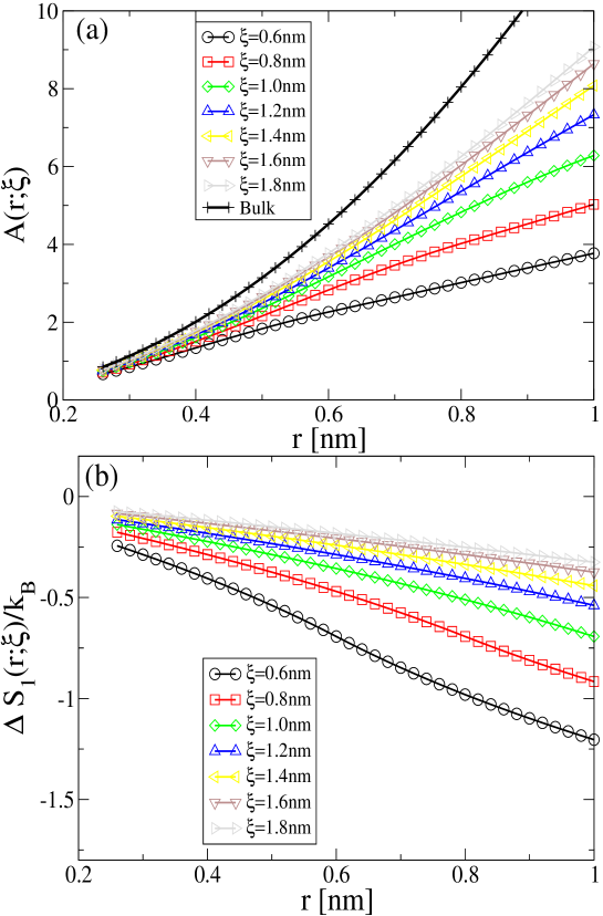
Figure S2: (a) Effective average area traced by a particle for a fixed distance $r$ from a reference particle, and (b) Entropy change $\Delta S_{1}(r;\xi)$ as a function of $r$ for different confinement widths.

References

- (1) Yun-Chi Tang, Hung-Chun Chang, and Annette Roeben et.al.,Cell 125, 903 (2006).
- (2) F. Ulrich Hartl, Andreas Bracher, and Manajit Hayer-Hartl,Nature 475, 324 (2011).
- (3) Jianyang Wu, Jianying He, Ole Torsæter, Zhiliang Zhang, Soc. Petr. Engg. (SPE) 156995 (2013).
- (4) P. Kumar, S. V. Buldyrev, F. W. Starr, H. E. Stanley Phys. Rev. E 72, 051503 (2005).
- (5) K. Koga, H. Tanaka, and X. C. Zeng,Nature 408, 564 (2000).
- (6) K. Koga, G. T. Gao, H. Tanaka, and X. C. Zeng, Nature 412, 802 (2001).
- (7) T. M. Truskett and P. G. Debenedetti, J. Chem. Phys. 114, 2401 (2001).
- (8) R. Zangi and A. E. Mark,Phys. Rev. Lett. 91, 0255502 (2003).
- (9) D Corradini, P Gallo, and M Rovere, J. Chem. Phys. 128, 244508 (2008).
- (10) J. C. Johnson, N. Kastelowitz, and V. Molinero, J. Chem. Phys. 133, 154516 (2010).
- (11) S. Han, M. Y. Choi, P. Kumar, and H. E. Stanley, Nature 6, 685 (2010).
- (12) S.-H. Chen, L. Liu, E. Fratini, P. Baglioni, A. Faraone, and E. Mamontov, Proc. Nat. Acad.Sci. USA 103, 9012 (2006).
- (13) L. Liu et al., Phys. Rev. Lett. 95, 117802 (2005).
- (14) N. Giovambattista, P.G. Debenedetti and P.J. Rossky,J. Phys. Chem. C 111, 1323 (2007).
- (15) N. Giovambattista, P.J. Rossky and P.G. Debenedetti, Phys. Rev. Lett. 102, 050603 (2009).
- (16) F. Mallamace, C. Corsaor, D. Mallamace, P. Baglioni, H. E. Stanley, and S.-H. Chen, J. Phys. Chem. 115 14280 (2011).
- (17) U. Raviv, P. Laurat, and J. Klein,Nature 413, 51 (2001).
- (18) J. Bai and x. C. Zeng, Proc. Natl. Acad. Sci. 109, 210240 (2012).
- (19) P. K. Varma, R. Saha, R. K. Mitra, and S. K. Pal, Soft Matter 6, 5971 (2010).
- (20) P. M. Wiggins, Physica A. Statistical Mechanics and Its Applications 238, 113 (1997).
- (21) K. Lum, D. Chandler, and J. D. Weeks, J. Phys. Chem. B 103, 4590 (1999).
- (22) H. S. Asbaugh, T. M. Truskett, and P. G. Debenedetti, J. Chem. Phys. 116, 2907 (2002).
- (23) K. A. Dill, T. M. Truskett, V. Vlachy, and B. Harbar-Lee, Annu. Rev. Biophys. Biomol. Struct. 34 173 (2005).
- (24) S. Garde, G. Hummer, A. E. Garcia, M. E. Paulaitis, and L. R. Pratt,Phys. Rev. Lett. 77, 4966 (1996).
- (25) S. V. Buldyrev, P. Kumar, P. G. Debenedetti, P. Rossky, and H. E. Stanley, Proc. Nat. Acad. Sci. USA 104, 20177 (2007).
- (26) R. Zhou, B. J. Berne, and R. Germain, Proc. Nat. Acad. Sci. 98, 14931 (2001); M. Tarek and D. J. Tobias, Phys. Rev. Lett. 89, 275501 (2002).
- (27) M. R. Walsh, C. A. Koh, E. D. Sloan, A. K. Sum, D. T. Wu, Science 326, 1095 (2009).
- (28) R. Battino, in IUPAC Solubility Data series, ed. W. Hayduk, Pergamon Press, Oxford 1982, vol. 9 pp. 1-2.
- (29) R. Battino, in IUPAC Solubility Data series, ed. W. Hayduk, Pergamon Press, Oxford 1986, vol. 24, pp. 16-17.
- (30) R. Battino, in IUPAC Solubility Data series, ed. H. L. Clever and C. L. Young, Pergamon Press, Oxford, 1987, vol. 27/28, pp. 16-17.
- (31) P. G. Debenedetti, S. Sarupria, Science 326, 1070 (2009).
- (32) F. Mallamace, P. Baglioni, C. Corsaro, S.-H. Chen, D. Mallamace, C. Vasi, H. E. Stanley, J. Chem. Phys. 141 165104 (2014).
- (33) E. D. Sloan, C. A. Koh, CRC Press, Boca Raton, FL, ed. 3, 2008.
- (34) E. D. Sloan, Nature 426, 353 (2003).
- (35) M. W. Mahoney and W. L. Jorgensen, J. Chem. Phys. 112, 8910 (2000).
- (36) M. W. Mahoney and W. L. Jorgensen, J. Chem. Phys. 114, 363 (2001).
- (37) S. Pronk, S. Páll, Roland Schulz, et. al. Bioinformatics 29 845-854 (2013).
- (38) D.A. McQuarrie, Statistical mechanics, Harper and ROW, New York, 1976.
- (39) J. van Eerden, W. J. Briel, S. Harkema, and D. Feil, Chem. Phys. Lett. 164, 370 (1989).
- (40) A. Baranyai and D. J. Evans, Phys. Rev. A 40, 3817 (1989).
- (41) P. Kumar, Z. Yan, L. Xu, M. G. Mazza, S. V. Buldyrev, S.-H. Chen, S. Sastry, and H. E. Stanley, Phys. Rev. Lett. 97, 177802 (2006).
- (42) A. Michaelides, and Karina Morgenstern, Nature Materials 6, 597 (2007).
- (43) J. Carrasco, A. Michaelides, M. Forster, S. Haq, R. Raval, and A. Hodgson, Nature Materials 8, 427 (2009).
- (44) J. C. Rasaiah, S. Garde, and Gerhard Hummer, Annu. Rev. Phys. Chem. 59, 713 (2008).
- (45) Water: A Comprehensive Treatise, Vol. 1. The Physics and Physical Chemistry of Water, Editor: F. Frank, Plenum Press, New York (1972).
- (46) P. G. Debenedetti and H. E. Stanley, Physics Today 56, 40 (2003).
- (47) R. Zangi, J. Phys.: Condens. Mat. 16, S5371 (2004).
- (48) K. Koga, J. Chem. Phys. 118, 7973 (2003).
- (49) R. Zangi and A. E. Mark, J. Chem. Phys. 120, 7123 (2004).
- (50) P. Scheidler, W. Kob, and K. Binder, Europhys. Lett. 59, 701 (2002).
- (51) S. Han, P. Kumar, and H. E. Stanley, Phys. Rev. E 77, 030201(R) (2008).
- (52) S. Han, P. Kumar, and H. E. Stanley, Phys. Rev. E 79, 041202 (2009).
- (53) G. Hummer, S. Garde, A. E. Garcia, and L. R. Pratt, Chemical Physics 258, 349 (2000).
- (54) A. Kalra, S. Garde, and G. Hummer, Proc. Natl. Acad. Sci. USA. 100, 10175 (2003).
- (55) I. Hanasaki and A. Nakatani, J. Chem. Phys. 124, 174714 (2006).
- (56) P. Liu, E. Harder, and B. J. Berne, J. Phys. Chem. B 108, 6595 (2004).
- (57) J. P. Hansen and I. R. McDonald, Theory of Simple Liquids, Academic Press, London, (1996).
- (58) R. J. Ellis, Nature 442, 360 (2006).