Sparse Distance Weighted Discrimination

Abstract

Distance weighted discrimination (DWD) was originally proposed to handle the data piling issue in the support vector machine. In this paper, we consider the sparse penalized DWD for high-dimensional classification. The state-of-the-art algorithm for solving the standard DWD is based on second-order cone programming, however such an algorithm does not work well for the sparse penalized DWD with high-dimensional data. In order to overcome the challenging computation difficulty, we develop a very efficient algorithm to compute the solution path of the sparse DWD at a given fine grid of regularization parameters. We implement the algorithm in a publicly available R package sdwd. We conduct extensive numerical experiments to demonstrate the computational efficiency and classification performance of our method.
Key words: High-dimensional classification, SVM, DWD.

1 Introduction

The support vector machine (SVM) (Vapnik, 1995) is a widely used modern classification method. In the standard binary classification problem, training dataset consists of $n$ pairs, $\{(\mathbf{x}_{i},y_{i})\}_{i=1}^{n}$, where $\mathbf{x}_{i}\in\mathbb{R}^{p}$ and $y_{i}\in\{-1,1\}$. The linear SVM seeks a hyperplane $\{\mathbf{x}:\beta_{0}+\mathbf{x}^{T}\boldsymbol{\beta}=0\}$ which maximizes the smallest margin of all data points:

$$\operatorname*{arg\ max}_{\beta_{0},\boldsymbol{\beta}}\;\;\;\; \min_{i}d_{i},$$

subject to $$d_{i}=y_{i}(\beta_{0}+\mathbf{x}_{i}^{T}\boldsymbol{\beta})+\eta_{i}\geq 0,\ \forall i,$$

$$\eta_{i}\geq 0,\ \forall i,\ \sum_{i=1}^{n}\eta_{i}\leq c,\ ||\boldsymbol{\beta}||_{2}^{2}=1,$$ (1.1)

where $d_{i}$ is defined as the margin of the $i$th data point, $\eta_{i}$’s are slack variables introduced to ensure all margins non-negative, and $c>0$ is a tuning parameter controlling the overlap. By using a kernel trick, the SVM can also produce nonlinear decision boundaries by fitting an optimal separating hyperplane in the extended kernel feature space. The readers are referred to Hastie et al. (2009) for a more detailed explanation of the SVM.

Marron et al. (2007) noticed that when the SVM is applied on some data with $n<p$, many data points lie on two hyperplanes parallel to the decision boundary. Marron et al. (2007) referred to this phenomenon as data pilling and claimed that the data pilling can “affect the generalization performance of SVM”. To overcome this issue, Marron et al. (2007) proposed a new method called the distance weighted discrimination (DWD), which finds a separating hyperplane minimizing the sum of the inverse margins of all data points:

$$\operatorname*{arg\ min}_{\beta_{0},\boldsymbol{\beta}}\;\;\;\; \sum_{i}{1}/{d_{i}},$$

subject to $$d_{i}=y_{i}(\beta_{0}+\mathbf{x}_{i}^{T}\boldsymbol{\beta})+\eta_{i}\geq 0,\ \forall i,$$

$$\eta_{i}\geq 0,\ \forall i,\ \sum_{i}\eta_{i}\leq c,\ ||\boldsymbol{\beta}||_{2}^{2}=1.$$ (1.2)

The initial version of Marron et al. (2007) also mentioned the sum of the inverse margins $\sum_{i}1/d_{i}$ could be also replaced by $\sum_{i}1/d_{i}^{q}$, the $q$th power of the inverse margins, and this generalized version was used as the definition of the DWD in Hall et al. (2005). Marron et al. (2007) asserted the DWD can avoid the data piling and thereby improve the generalizability. One example [see the group 2 of Figure 3 in Marron et al. (2007)] shows that the DWD has about 5% prediction error whereas the SVM does 15%. Enhancement of the DWD over the SVM can also be exemplified in Hall et al. (2005) through a novel geometric view. As for the computation of the DWD, Marron et al. (2007) observed that the DWD is an application of the second-order cone programming and thus can be solved by the primal-dual interior-point methods. The algorithm has been implemented in both Matlab code http://www.unc.edu/~marron/marron_software.html and an R package DWD (Huang et al., 2012).

In this paper we focus on classification with high-dimensional data where the number of covariates is much larger than the sample size. The standard SVM and DWD are not suitable tools for high-dimensional classification for two reasons. First, based on the scientific hypothesis that only a few important variables affect the outcome, a good classifier for high-dimensional classification should have the ability to select important variables and discard irrelevant ones. However, the standard SVM and DWD use all variables and do not conduct variable selection. Second, because these two classifiers use all variables, they may have very poor classification performance. As explained in Fan and Fan (2008), the bad performance is caused by the error accumulation when estimating too many noise variables in the classifier. Owing to these two considerations, sparse classifiers are generally preferred for high-dimensional classification. In the literature, some penalties have been applied to the SVM to produce sparse SVMs such as the $\ell_{1}$ SVM (Bradley and Mangasarian, 1998; Zhu et al., 2004), the SCAD SVM (Zhang et al., 2006), and the elastic-net penalized SVM (Wang et al., 2006).

In this work we consider sparse penalized DWD for high dimensional classification. The standard DWD uses the $\ell_{2}$ penalty and can be solved by the second-order cone programming. However, the sparse DWD is computationally more challenging and requires a different computing algorithm. To cope with the computational challenges associated with the sparse penalty and high-dimensionality, we derive an efficient algorithm to solve the sparse DWD by combining majorization-minimization principle and coordinate-descent. We have implemented the algorithm in an R package sdwd. To give a quick demonstration here, we use the prostate cancer data [Singh et al. (2002), 102 observations and 6033 genes] as an example. The left panel of Figure 1 depicts the solution paths of the elastic-net penalized DWD, and sdwd only took 0.453 second to compute the whole solution path. As comparison, we also used the code in Wang et al. (2006) to compute the solution path of the elastic-net penalized SVM. We observed that the timing of the sparse SVM was about 290 times larger than that of the sparse DWD.

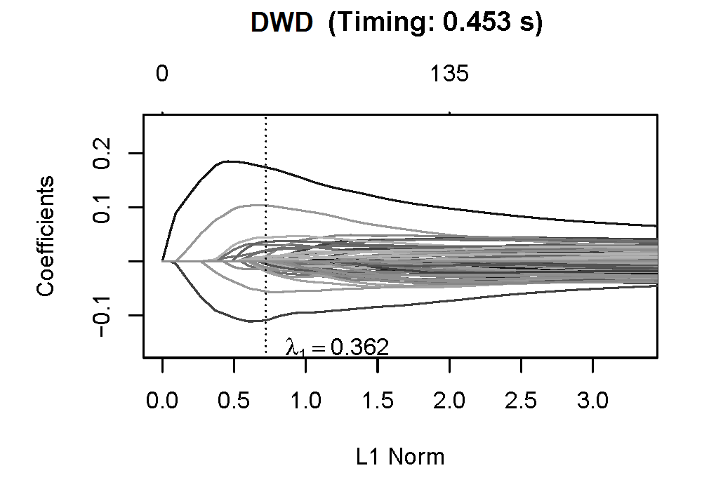
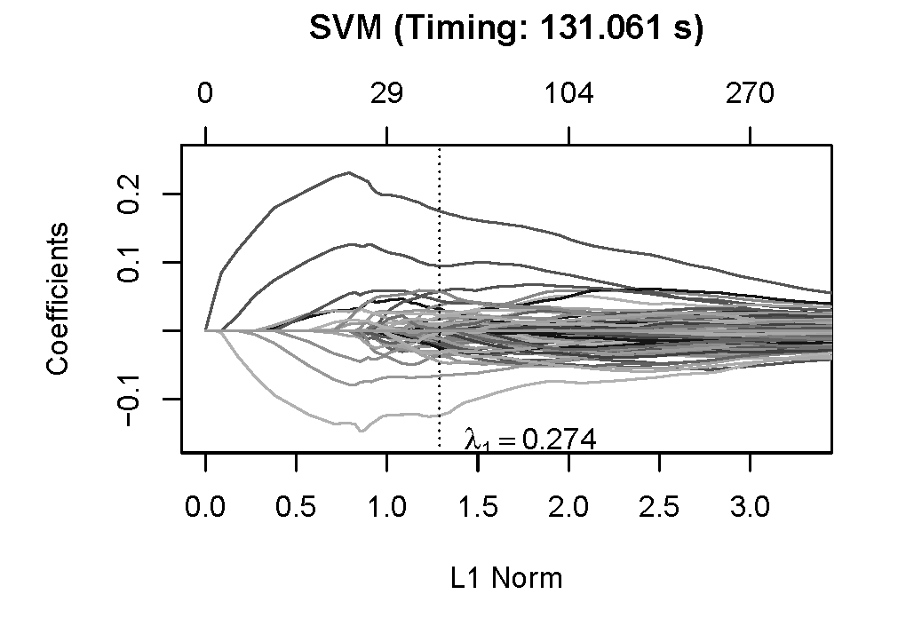
Figure 1: The solution paths for the prostate data ($n=102$, $p=6033$) using the elastic-net DWD and the elastic-net SVM. In every method, $\lambda_{2}$ is fixed to be 1. The dashed vertical lines indicate the $\lambda_{1}$ selected by the five-folder cross validation. Both timings are averaged over 10 runs.

2 Sparse DWD

In this section we present several sparse penalized DWDs. Our formulation follows the $\ell_{1}$ SVM (Zhu et al., 2004). Thus, we first review the derivation process of the $\ell_{1}$ SVM. The standard SVM (1.1) is often rephrased as the following quadratic programming problem (Hastie et al., 2009):

$$\operatorname*{arg\ min}_{\beta_{0},\boldsymbol{\beta}} ||\boldsymbol{\beta}||^{2}_{2}$$

subject to $$y_{i}(\beta_{0}+\mathbf{x}_{i}^{T}\boldsymbol{\beta})+\eta_{i}\geq 1,\ \forall i,$$

$$\eta_{i}\geq 0,\ \forall i,\ \sum_{i=1}^{n}\eta_{i}\leq c.$$

Moreover, the above constrained minimization problem has an equivalent loss+penalty formulation (Hastie et al., 2009):

$$\operatorname*{arg\ min}_{\beta_{0},\boldsymbol{\beta}}\dfrac{1}{n}\sum_{i=1}^{n}\left[1-y_{i}(\beta_{0}+\mathbf{x}_{i}^{T}\boldsymbol{\beta})\right]_{+}+\dfrac{\lambda_{2}}{2}||\boldsymbol{\beta}||^{2}_{2}.$$

The loss function $[1-t]_{+}=\max(1-t,\ 0)$ is the so-called hinge loss in the literature. For the high-dimensional setting, the standard SVM uses all variables because of the $\ell_{2}$ norm penalty used therein. As a result, its performance can be very poor. Zhu et al. (2004) proposed the $\ell_{1}$-norm SVM to fix this issue:

$$\operatorname*{arg\ min}_{\beta_{0},\boldsymbol{\beta}}\dfrac{1}{n}\sum_{i=1}^{n}\left[1-y_{i}(\beta_{0}+\mathbf{x}_{i}^{T}\boldsymbol{\beta})\right]_{+}+\lambda_{1}||\boldsymbol{\beta}||_{1}.$$

Similarly, we can propose the $\ell_{1}$ penalized DWD. It has been shown that the standard DWD also has a loss+penalty formulation (Liu et al., 2011):

$$\operatorname*{arg\ min}_{\beta_{0},\boldsymbol{\beta}}\dfrac{1}{n}\sum_{i=1}^{n}V\left(y_{i}(\beta_{0}+\mathbf{x}_{i}^{T}\boldsymbol{\beta})\right)+\dfrac{\lambda_{2}}{2}||\boldsymbol{\beta}||^{2}_{2},$$

where the loss function is given by

$$V(u)=\begin{cases}1-u,\;&\text{ if }u\leq 1/2,\\ 1/(4u),\;&\text{ if }u>1/2.\end{cases}$$

Similar to the $\ell_{1}$ SVM, we replace the $\ell_{2}$ norm penalty with the $\ell_{1}$ norm penalty in order to achieve sparsity in the DWD classifier. Hence, the $\ell_{1}$ DWD is defined by

$$\left(\hat{\beta}_{0}(\mathrm{lasso}),\hat{\boldsymbol{\beta}}(\mathrm{lasso})\right)=\operatorname*{arg\ min}_{\beta_{0},\boldsymbol{\beta}}\dfrac{1}{n}\sum_{i=1}^{n}V\left(y_{i}(\beta_{0}+\mathbf{x}_{i}^{T}\boldsymbol{\beta})\right)+{\lambda_{1}}||\boldsymbol{\beta}||_{1}.$$ (2.1)

The lasso penalized DWD classification rule is $\textrm{Sign}(\hat{\beta}_{0}(\mathrm{lasso})+\mathbf{x}^{T}\hat{\boldsymbol{\beta}}(\mathrm{lasso}))$.

Besides the $\ell_{1}$ norm penalty, we also consider the elastic-net penalty (Zou and Hastie, 2005). It is now well-known that the elastic-net often outperforms the lasso ($\ell_{1}$ norm penalty) in prediction. Wang et al. (2006) studied the elastic-net penalized SVM (DrSVM) and showed that the DrSVM performs better than the $\ell_{1}$ norm SVM. Similarly, we propose the elastic-net penalized DWD:

$$\left(\hat{\beta}_{0}(\mathrm{enet}),\hat{\boldsymbol{\beta}}(\mathrm{enet})\right)=\operatorname*{arg\ min}_{\beta_{0},\boldsymbol{\beta}}\dfrac{1}{n}\sum_{i=1}^{n}V(y_{i}(\beta_{0}+\mathbf{x}_{i}^{T}\boldsymbol{\beta}))+P_{\lambda_{1},\lambda_{2}}(\boldsymbol{\beta}),$$ (2.2)

where

$$P_{\lambda_{1},\lambda_{2}}(\boldsymbol{\beta})=\sum_{j=1}^{p}\left(\lambda_{1}|\beta_{j}|+\frac{\lambda_{2}}{2}\beta_{j}^{2}\right).$$

The elastic-net penalized DWD classification rule is $\textrm{Sign}(\hat{\beta}_{0}(\mathrm{enet})+\mathbf{x}^{T}\hat{\boldsymbol{\beta}}(\mathrm{enet}))$. Both $\lambda_{1}$ and $\lambda_{2}$ are important tuning parameters for regularization. In practice, $\lambda_{1}$ and $\lambda_{2}$ are chosen from finite grids by validation or cross-validation.

A further refinement of the elastic-net penalty is the adaptive elastic-net penalty (Zou and Zhang, 2009) where we replace the $\ell_{1}$ (lasso) penalty with the adaptive $\ell_{1}$ (lasso) penalty (Zou, 2006). The adaptive lasso penalty produces estimators with the oracle properties. The adaptive elastic-net enjoys the benefits of elastic-net and adaptive lasso. After fitting the elastic-net penalized DWD, we further consider the adaptive elastic-net penalized DWD:

$$\left(\hat{\beta}_{0}(\mathrm{aenet}),\hat{\boldsymbol{\beta}}(\mathrm{aenet})\right)=\operatorname*{arg\ min}_{\beta_{0},\boldsymbol{\beta}}\dfrac{1}{n}\sum_{i=1}^{n}V(y_{i}(\beta_{0}+\mathbf{x}_{i}^{T}\boldsymbol{\beta}))+\sum_{j=1}^{p}\left(\lambda_{1}\hat{\omega}_{j}|\beta_{j}|+\frac{\lambda_{2}}{2}\beta_{j}^{2}\right),$$ (2.3)

and the adaptive weights are computed by

$$\hat{\omega}_{j}=(|\hat{\beta}_{j}(\mathrm{enet})|+1/n)^{-1},$$

where $\hat{\beta}_{j}(\mathrm{enet})$ is the solution of $\beta_{j}$ in (2.2). The adaptive elastic-net penalized DWD classification rule is $\textrm{Sign}(\hat{\beta}_{0}(\mathrm{aenet})+\mathbf{x}^{T}\hat{\boldsymbol{\beta}}(\mathrm{aenet}))$.

3 Computation

The $\ell_{2}$ DWD was solved based on the second-order-cone programming; nevertheless, it is not trivial to generalize the algorithm to the $\ell_{1}$ DWD, and even more difficult to handle the elastic-net and the adaptive elastic-net penalties. In this section, we propose a completely different algorithm. We solve the solution paths of the sparse DWD by using the generalized coordinate descent (GCD) algorithm proposed by Yang and Zou (2013). We introduce the GCD algorithm in section 3.1, the implementation in section 3.2, and the strict descent property in section 3.3. The same algorithm solves all the $\ell_{1}$, the elastic-net, and adaptive elastic-net penalized DWDs, while only the elastic-net is focused in the discussion for the sake of presentation.

3.1 Derivation of the algoithm

Without loss of generality, we assume that the variables $\mathbf{x}_{j}$ are standardized: $\sum_{i=1}^{n}x_{ij}=0,\frac{1}{n}\sum_{i=1}^{n}x_{ij}^{2}=1$, for $j=1,\ldots,p$. We fix $\lambda_{1}$ and $\lambda_{2}$ and let $u_{i}=y_{i}(\tilde{\beta}_{0}+\mathbf{x}_{i}^{T}\tilde{\boldsymbol{\beta}})$. We focus on $\beta_{j}$’s first. For each $\beta_{j}$, we define the coordinate-wise update function:

$$F(\beta_{j}|\boldsymbol{\tilde{\beta}},\tilde{\beta}_{0}) =\frac{1}{n}\sum_{i=1}^{n}V\left(u_{i}+y_{i}x_{ij}(\beta_{j}-\tilde{\beta}_{j})\right)+p_{\lambda_{1},\lambda_{2}}(\beta_{j}).$$ (3.1)

Then the standard coordinate descent algorithm suggests cyclically updating

$$\hat{\beta}_{j}=\operatorname*{arg\ min}_{\beta_{j}}F(\beta_{j}|\tilde{\beta}_{0},\tilde{\boldsymbol{\beta}})$$ (3.2)

for each $j=1,\ldots,p$. However, (3.2) does not have a closed-form solution. The GCD algorithm solves this issue by adopting the MM principle (Hunter and Lange, 2004). We approximate the $F$ function by a quadratic function

$$Q(\beta_{j}|\boldsymbol{\tilde{\beta}},\tilde{\beta}_{0})=\frac{\sum_{i=1}^{n}V(u_{i})}{n}+\frac{\sum_{i=1}^{n}V^{\prime}(u_{i})y_{i}x_{ij}}{n}(\beta_{j}-\tilde{\beta}_{j})+2(\beta_{j}-\tilde{\beta}_{j})^{2}+p_{\lambda_{1},\lambda_{2}}(\beta_{j}).$$ (3.3)

Then we update $\tilde{\beta_{j}}$ by $\tilde{\beta}_{j}^{\mathrm{new}}$, the closed-form minimizer of (3.3):

$$\tilde{\beta}_{j}^{\text{new}}=\dfrac{S\left(M\tilde{\beta}_{j}-\frac{1}{n}\sum_{i=1}^{n}V^{\prime}(u_{i})y_{i}x_{ij},\lambda_{1}\right)}{4+\lambda_{2}},$$ (3.4)

where $S(z,r)=\text{sign}(z)(|z|-r)_{+}$ is the soft-thresholding operator (Donoho and Johnston, 1994) and $\omega_{+}=\max(\omega,0)$ is the positive part of $\omega$.

With the intercept similarly updated, Algorithm 1 summarizes the details of the GCD algorithm.

1. Initialize $(\tilde{\beta}_{0},\tilde{\boldsymbol{\beta}})$.

2. Cyclic coordinate descent, for $j=1,2,\ldots,p$:

   1. Compute $u_{i}=y_{i}(\tilde{\beta}_{0}+\mathbf{x}_{i}^{\intercal}\tilde{\boldsymbol{\beta}})$.

   2. Compute $\tilde{\beta}_{j}^{\text{new}}=\frac{1}{4+\lambda_{2}}\cdot S\left(4\tilde{\beta}_{j}-\frac{1}{n}\sum_{i=1}^{n}V^{\prime}(u_{i})y_{i}x_{ij},\lambda_{1}\right).$

   3. Set $\tilde{\beta}_{j}=\tilde{\beta}_{j}^{\text{new}}$.

3. Update the intercept term:

   1. Compute $u_{i}=y_{i}(\tilde{\beta}_{0}+\mathbf{x}_{i}^{T}\tilde{\boldsymbol{\beta}})$.

   2. Compute $\tilde{\beta}_{0}^{\text{new}}=\tilde{\beta}_{0}-{\sum_{i=1}^{n}V^{\prime}(u_{i})y_{i}}/{(4n)}.$

   3. Set $\tilde{\beta}_{0}=\tilde{\beta}_{0}^{\text{new}}$.

4. Repeat steps 2-3 until convergence of $(\tilde{\beta}_{0},\tilde{\boldsymbol{\beta}})$.

Algorithm 1 The GCD algorithm for the sparse DWD

3.2 Implementation

We have implemented Algorithm 1 in an R package sdwd. We exploit the warm-start, the strong rule, and the active set trick to increase the algorithm speeding. In our implementation, $\lambda_{2}$ is pre-chosen and we compute the solution path as $\lambda_{1}$ varies.

First, we adopt the warm-start to lead to a faster and more stable algorithm (Friedman et al., 2007). We compute the solutions at a grid of $K$ decreasing $\lambda_{1}$ values, starting at the smallest $\lambda_{1}$ value such that $\boldsymbol{\tilde{\beta}}=0$. Denote these grid points by $\lambda_{1}^{[1]},\ldots,\lambda_{1}^{[K]}$. With the warm-start trick, we can use the solution at $\lambda_{1}^{[k]}$ as the initial value (the warm-start) to compute the solution at $\lambda_{1}^{[k+1]}$.

Specifically, to find $\lambda_{1}^{[1]}$, we fit a model with a sufficiently large $\lambda_{1}$ and thus $\boldsymbol{\tilde{\beta}}=0$. Let $\hat{\beta}_{0}$ be the estimate of the intercept. By the KKT conditions, $\frac{1}{n}\max_{j}\left|\sum_{i=1}^{n}V^{\prime}(\hat{\beta}_{0})y_{i}x_{ij})\right|\leq\lambda_{1}$, so we can choose

$$\lambda_{1}^{[1]}=\frac{1}{n}\max_{j}\left|\sum_{i=1}^{n}V^{\prime}(\hat{\beta}_{0})y_{i}x_{ij})\right|.$$

Generally, we use $K=100$, and $\lambda_{1}^{[100]}=\epsilon\lambda_{1}^{[1]}$, where $\epsilon=10^{-4}$ when $n<p$ and $\epsilon=10^{-2}$ otherwise. All the other grid points are placed to uniformly distribute on a log scale.

Second, we follow the strong rule (Tibshirani et al., 2010) to improve the computational speed. Suppose $\boldsymbol{\tilde{\beta}}^{[k]}$ and $\tilde{\beta}_{0}^{[k]}$ are the solutions at $\lambda_{1}^{[k]}$. After we solve $\boldsymbol{\tilde{\beta}}^{[k]}$ and $\tilde{\beta}_{0}^{[k]}$, the strong rule claims that any $j\in\{1,\ldots,p\}$ satisfying

$$\left|\frac{1}{n}\sum_{i=1}^{n}V^{\prime}(y_{i}(\hat{\beta}_{0}^{[k]}+x_{i}^{T}\boldsymbol{\hat{\beta}}^{[k]}))y_{i}x_{ij}\right|<2\lambda_{1}^{[k+1]}-\lambda_{1}^{[k]}$$ (3.5)

is likely to be inactive at $\lambda_{1}^{[k+1]}$, i.e., $\hat{\beta}_{j}^{[k+1]}=0$. Let $\mathcal{D}$ be the collection of $j$ which satisfies (3.5), and its compliment $\mathcal{D}^{C}=\{1,\ldots,p\}\backslash\mathcal{D}$. We call $\mathcal{D}^{C}$ the survival set. If the strong rule guesses correctly, the variables contained in $\mathcal{D}$ are discarded, and we only apply Algorithm 1 to repeat the coordinate descent in the survival set $\mathcal{D}^{C}$. After computing the solution $\hat{\beta}_{0}$ and $\boldsymbol{\hat{\beta}}$, we need to check whether some variables are incorrectly discarded. We check this by the KKT condition,

$$\left|\dfrac{1}{n}\sum_{i=1}^{n}V^{\prime}(y_{i}(\hat{\beta}_{0}+x_{i}^{T}\boldsymbol{\hat{\beta}}))y_{i}x_{ij}\right|\leq\lambda_{1}.$$ (3.6)

If no $j\in\mathcal{D}$ violates (3.6), $\hat{\beta}_{0}$ and $\boldsymbol{\hat{\beta}}$ are the solutions at $\lambda_{1}^{[k+1]}$. We rephrase them as $\tilde{\beta}_{0}^{[k+1]}$ and $\boldsymbol{\tilde{\beta}}^{[k+1]}$. Otherwise, any incorrectly discarded variable should be added to the survival set $\mathcal{D}^{C}$. We update $\mathcal{D}$ by $\mathcal{D}=\mathcal{D}/U$ where

$$U=\left\{j:j\in\mathcal{D}\text{ and }\left|\dfrac{1}{n}\sum_{i=1}^{n}V^{\prime}(y_{i}(\hat{\beta}_{0}+x_{i}^{T}\boldsymbol{\hat{\beta}}))y_{i}x_{ij}\right|>\lambda_{1}\right\}.$$

After each update of $\mathcal{D}$, some incorrectly discarded variables are added back to the survival set.

Third, the active set is also used to boost the algorithm speed. After we apply Algorithm 1 on the survival set $\mathcal{D}^{C}$, we only apply the coordinate descent on a subset $S$ of $\mathcal{D}^{C}$ till convergence, where $S=\left\{j:j\in\mathcal{D}^{C}\text{ and }\beta_{j}\neq 0\right\}$. Then another cycle of coordinate descent is run on $\mathcal{D}^{C}$ to investigate if the active set $S$ changes. We finish the algorithm if no changes in $S$; otherwise, we update the active set $S$ and repeat the process.

In Algorithm 1, the margin $u_{i}$ can be updated conveniently: if $\beta_{j}$ is updated by $\beta_{j}^{\text{new}}$, we update $u_{i}$ by $u_{i}+y_{i}x_{ij}(\beta_{j}^{\text{new}}-\beta_{j})$.

Last, the default convergence rule in sdwd is $4(\tilde{\beta}_{j}^{\mathrm{new}}-\tilde{\beta}_{j})^{2}<10^{-8}$ for all $j=0,1,\ldots,p$.

3.3 The strict descent property of Algorithm 1

Yang and Zou (2013) showed the GCD algorithm enjoys descent property. In this section, we also show the GCD algorithm has a stronger statement, the strict descent property, when the GCD is used to solve the sparse DWD. We first elaborate the following majorization result, whose proof is deferred in the appendix.

Lemma 1.

$F(\beta_{j}|\boldsymbol{\tilde{\beta}},\tilde{\beta}_{0})$ is the coordinate-wise update function defined in (3.1), and $Q(\beta_{j}|\boldsymbol{\tilde{\beta}},\tilde{\beta}_{0})$ is the surrogate function defined in (3.3). We have (3.7) and (3.8):

$$F(\beta_{j}|\boldsymbol{\tilde{\beta}},\tilde{\beta}_{0}) =Q(\beta_{j}|\boldsymbol{\tilde{\beta}},\tilde{\beta}_{0}),\ \text{if}\ \beta_{j}=\tilde{\beta}_{j},$$ (3.7)

$$F(\beta_{j}|\boldsymbol{\tilde{\beta}},\tilde{\beta}_{0}) <Q(\beta_{j}|\boldsymbol{\tilde{\beta}},\tilde{\beta}_{0}),\ \text{if}\ \beta_{j}\neq\tilde{\beta}_{j}.$$ (3.8)

Given $\tilde{\beta}_{j}^{\text{new}}=\operatorname*{arg\ min}_{\beta_{j}}Q(\beta_{j}|\tilde{\beta}_{0},\tilde{\boldsymbol{\beta}})$, and assuming $\tilde{\beta}_{j}^{\text{new}}\neq\tilde{\beta}_{j}$, (3.7) and (3.8) imply the strict descent property of the GCD algorithm: $F(\tilde{\beta}_{j}^{\text{new}}|\boldsymbol{\tilde{\beta}},\tilde{\beta}_{0})<F(\tilde{\beta}_{j}|\boldsymbol{\tilde{\beta}},\tilde{\beta}_{0})$. It is because $F(\tilde{\beta}_{j}^{\text{new}}|\boldsymbol{\tilde{\beta}},\tilde{\beta}_{0})<Q(\tilde{\beta}_{j}^{\text{new}}|\boldsymbol{\tilde{\beta}},\tilde{\beta}_{0})<Q(\tilde{\beta}_{j}|\boldsymbol{\tilde{\beta}},\tilde{\beta}_{0})=F(\tilde{\beta}_{j}|\boldsymbol{\tilde{\beta}},\tilde{\beta}_{0})$. Note that the original GCD paper only showed $F(\tilde{\beta}_{j}^{\text{new}}|\boldsymbol{\tilde{\beta}},\tilde{\beta}_{0})\leq F(\tilde{\beta}_{j}|\boldsymbol{\tilde{\beta}},\tilde{\beta}_{0})$.

The arguments above prove that the objective function $F$ strictly decreases after updating all variables in a cycle, unless the solution does not change after each update. If this is the case, the algorithm stops. We show that the algorithm must stop at the right answer. Assuming $\tilde{\beta}_{j}=\tilde{\beta}_{j}^{\text{new}}$ for all $j$, (3.4) implies:

$$\tilde{\beta}_{j}=\dfrac{S(4\tilde{\beta}_{j}-\frac{1}{n}\sum_{i=1}^{n}V^{\prime}(u_{i})y_{i}x_{ij},\lambda_{1})}{4+\lambda_{2}}.$$

A straightforward algebra can show that for all $j$,

$$\dfrac{1}{n}\sum_{i=1}^{n}V^{\prime}(u_{i})y_{i}x_{ij}+\lambda_{1}\text{sign}(\beta_{j})+\lambda_{2}\beta_{j}=0,\ \text{if }\beta_{j}\neq 0;$$

$$\left|\dfrac{1}{n}\sum_{i=1}^{n}V^{\prime}(u_{i})y_{i}x_{ij}\right|\leq\lambda_{1},\ \text{if }\beta_{j}=0,$$

which is exactly the KKT conditions of the original objective function (2.2). In conclusion, if the objective function does not change after a cycle, the algorithm necessarily converges to the correct solution satisfying the KKT condition.

4 Simulation

The simulation in this section aims to support the following three points: (1) the sparse DWD has highly competitive prediction accuracy with the sparse SVM and the sparse logistic regression; (2) the adaptive elastic-net penalized DWD performs the best in variable selection; (3) for the prediction accuracy, no single method among the $\ell_{1}$, the elastic-net, and the adaptive elastic-net penalized DWDs dominate the others in all situations.

In this section, the response variables of all the data are binary. The dimension $p$ of the variables $\mathbf{x}_{i}$ is always 3000. Within each example, our simulated data consist of a training set, an independent validation set, and an independent test set. The training set contains 50 observations: 25 of them are from the positive class and the other 25 from the negative class. Models are fitted on the training data only, and we use an independent validation set of 50 observations to select the tuning parameters: $\lambda_{2}$ is selected from $10^{-4}$, $10^{-3}$, $10^{-2}$, $0.1$, 1, 5, and 10; $\lambda_{1}$ is searched along the solution paths. We compared the prediction accuracy (in percentage) on another independent test data set of 20,000 observations.

We followed Marron et al. (2007) to generate the first two examples. In example 1, the positive class is a random sample from $N_{p}(\boldsymbol{\mu}_{+},\boldsymbol{I}_{p})$, where $\boldsymbol{I}_{p}$ is the $p$ by $p$ identity matrix and $\boldsymbol{\mu}_{+}$ has all zeros except for $2.2$ at the first dimension; the negative class is from $N_{p}(\boldsymbol{\mu}_{-},\boldsymbol{I}_{p})$ with $\boldsymbol{\mu}_{-}=-\boldsymbol{\mu}_{+}$. In example 2, $80\%$ of the data are generated from the same distributions as example 1; for the other $20\%$ of the data, the positive class is drawn from $N_{p}(\boldsymbol{\mu}_{+},\boldsymbol{I}_{p})$ and negative class $N_{p}(-\boldsymbol{\mu}_{+},\boldsymbol{I}_{p})$ where $\boldsymbol{\mu}_{+}=(100,500,0,\ldots,0)$. We obtained the other three examples following Wang et al. (2006). In example 3, the positive class has a normal distribution with mean $\boldsymbol{\mu}_{+}$ and covariance $\boldsymbol{\Sigma}=\boldsymbol{I}_{p\times p}$, where $\boldsymbol{\mu}_{+}$ has 0.7 in the first five covariates and 0 in others; the negative class has the same distribution except for a different mean $\boldsymbol{\mu}_{-}=-\boldsymbol{\mu}_{+}$. In example 4 and 5, we consider the cases where the relevant variables are correlated. Two classes have the same distributions except for the covariance,

$$\boldsymbol{\Sigma}=\left(\begin{array}[]{ccc}\boldsymbol{\Sigma}_{5\times 5}^{\star}&\boldsymbol{0}_{5\times(p-5)}\\ \boldsymbol{0}_{(p-5)\times 5}&\boldsymbol{I}_{(p-5)\times(p-5)}\end{array}\right).$$

In example 4, the diagonal elements of $\boldsymbol{\Sigma}^{\star}$ are 1 and the off-diagonal elements are all equal to $0.7$. In example 5, the $(i,j)$th element of $\boldsymbol{\Sigma}^{\star}$ equals $0.7^{|i-j|}$.

We compared the sparse DWD with the sparse SVM and the sparse logistic regression. Both the DWD and the logistic regression use the $\ell_{1}$, the elastic-net and the adaptive elastic-net penalties. We used R packages sdwd and gcdnet (Yang and Zou, 2013) to compute the sparse DWDs and the sparse logistic regressions respectively. The $\ell_{1}$ and the elastic-net SVMs were solved by using the code from Wang et al. (2006) which does not handle the adaptive elastic-net penalty. Table 1 presents the prediction accuracy results. In the first two examples, the $\ell_{1}$ DWD and the $\ell_{1}$ logistic regression perform the best. We attribute this good performance to the only one nonzero variable in the data, despite $20\%$ of outliers in example 2. In example 3, 4, and 5, we increase the number of nonzero variables to five. For all models, the elastic-net and the adaptive elastic-net penalties have similar performance, and both of them dominate the $\ell_{1}$ penalties. The elastic-net DWD produces the least prediction error in example 4 and 5. Table 3 compares the variable selection. In all cases, the adaptive elastic-net penalties address all relevant variables with relatively few mistakes. The $\ell_{1}$ penalties share similar performance in the first two examples.

Table 1: Comparisons of mis-classification percentage on 300 training data, 300 validation data, and 20,000 test data, based on 200 replicates. The numbers in parentheses are the standard errors. For each example, the methods with the best performance are marked by black boxes.

		DWD				SVM			logistic
		$\ell_{1}$	enet	aenet		$\ell_{1}$	enet		$\ell_{1}$	enet	aenet
	Example 1	1.42	1.47	1.44		1.46	1.50		1.42	1.46	1.44
	Bayes: 1.39	(0.01)	(0.02)	(0.01)		(0.01)	(0.02)		(0.01)	(0.02)	(0.02)
	Example 2	1.14	1.15	1.13		1.16	1.16		1.11	1.14	1.15
	Bayes: 1.11	(0.01)	(0.01)	(0.01)		(0.01)	(0.01)		(0.01)	(0.01)	(0.02)
	Example 3	6.41	6.25	6.21		6.45	6.15		6.40	6.21	6.22
	Bayes: 5.88	(0.03)	(0.03)	(0.03)		(0.04)	(0.03)		(0.03)	(0.03)	(0.03)
	Example 4	22.05	21.48	21.54		22.03	21.56		22.00	21.54	21.64
	Bayes: 21.10	(0.07)	(0.07)	(0.05)		(0.06)	(0.05)		(0.06)	(0.06)	(0.06)
	Example 5	18.91	18.74	18.75		18.84	18.78		18.81	18.80	18.77
	Bayes: 18.03	(0.07)	(0.05)	(0.05)		(0.06)	(0.05)		(0.06)	(0.05)	(0.05)

Table 2: Comparisons of the variable selection. C is the number of selected nonzero variables, and IC is the number of zero variables incorrectly selected into the model. The results are the medians over 200 replicates.

	DWD							SVM					logistic
	$\ell_{1}$		enet		anet			$\ell_{1}$		enet			$\ell_{1}$		enet		aenet
	C	IC	C	IC	C	IC		C	IC	C	IC		C	IC	C	IC	C	IC
Example 1	1	0	1	2	1	0		1	0	1	4		1	0	1	4.5	1	0
Example 2	1	0	1	0	1	0		1	0	1	1		1	0	1	0	1	0
Example 3	5	0	5	5	5	0		5	0	5	2.5		5	1	5	7	5	0
Example 4	4	1	5	8.5	5	1.5		4	0	5	7		4	1	5	14	5	2
Example 5	4	1	5	3.5	5	0		4	0	5	2		4	1	5	6.5	5	0

5 Real Data Examples

In this section we analyze four benchmark data. The data Arcene was obtained from Frank and Asuncion (2010), the breast cancer data from Graham et al. (2010), the LSVT data from Tsanas et al. (2014), and the prostate cancer was from Singh et al. (2002). We randomly split each data with a ratio 1:1 into a training set and a test set. On the training set, we fit the sparse DWD with imposing the elastic-net and the adaptive elastic-net penalties. With the same tuning parameter candidates in the simulation, we used a five folder cross validation to find the best pair of $(\lambda_{1},\lambda_{2})$ incurring the least mis-classification rate. Then we investigated the prediction accuracy of the selected model on the test set. As comparisons, we considered the sparse SVM and the sparse logistic regression. Every method was trained and tuned in the same way as the sparse DWD. All numerical experiments were carried out on an Intel Core i7-3770 (3.40 GHz) processor.

In Table 3, we reported the average mis-classification percentage on the test set from 200 independent splits. We observe that the classifiers achieving the least error in these four datasets are the adaptive elastic-net logistic regression, the elastic-net SVM, the elastic-net and the adaptive elastic-net DWDs. We also find all the differences are not quite large. For the sparse DWD, we get the same message as Marron et al. (2007) concluded for the standard DWD: “it very often is competitive with the best of the others and sometimes is better.” We also notice that the computation of the sparse DWD is the fastest in almost all cases. The timing of the SVM is much longer than other methods. A possible explanation is that the SVM uses the non-differentiable hinge loss function which makes the GCD algorithm not suitable for solving the sparse SVM. So far, the best algorithm for the sparse SVM is a LARS type algorithm Wang et al. (2006), which is very different from the GCD algorithm for the sparse DWD and logistic regression. It has been observed that coordinate descent may be faster than the LARS algorithm for solving the lasso penalized least squares (Friedman et al., 2007).

Table 3: The mean mis-classification percentage and timings (in seconds) for four benchmark datasets. All the timings include the five-folder cross validation. The timings of adaptive elastic-net methods include computing the weights. The numbers in parentheses are the standard errors. For each data, the methods with the best prediction accuracy are marked by black boxes.

	Arcene			Breast			LSVT			Prostate
	$n=100$, $p=10000$			$n=42$, $p=22283$			$n=126$, $p=309$			$n=102$, $p=6033$
	error	time		error	time		error	time		error	time
enet DWD	34.43	123.41		26.50	58.40		16.01	8.28		10.22	28.18
	(0.56)	(5.16)		(1.00)	(1.90)		(0.34)	(0.23)		(0.30)	(0.95)
aenet DWD	34.60	200.19		26.86	116.12		15.92	13.72		10.26	39.25
	(0.57)	(9.24)		(1.00)	(3.78)		(0.34)	(0.29)		(0.26)	(1.24)
enet logistic	34.16	211.18		24.67	145.35		16.96	10.73		10.65	102.19
	(0.58)	(3.40)		(1.00)	(0.74)		(0.37)	(0.18)		(0.29)	(1.56)
aenet logistic	34.15	393.03		25.12	290.31		16.93	17.02		10.75	189.44
	(0.57)	(6.52)		(0.87)	(1.47)		(0.37)	(0.29)		(0.29)	(2.84)
enet SVM	35.10	7410.09		23.95	567.43		16.27	63.10		10.56	2508.94
	(0.67)	(1465.68)		(1.00)	(15.19)		(0.37)	(0.77)		(0.36)	(0.77)

6 Discussion

In this article, we have proposed the sparse DWD for high-dimensional classification and developed an efficient algorithm to compute its solution path. We have shown that the sparse DWD has competitive prediction performance with the sparse SVM and the sparse logistic regression and is often faster to compute with the help of our algorithm. Thus, the sparse DWD is a valuable addition to the toolbox for high-dimensional classification.

The generalized DWD defined in Hall et al. (2005) minimizes the $q$th power of the inverse margins. When $q=1$, it reduces to the usual DWD. For computation considerations, Marron et al. (2007) choose to fix $q=1$, because it leads to a second order cone programming problem. We have found that our algorithm can be readily used to solve the sparse generalized DWD with any positive $q$. In our numerical study we tried the generalized DWD with $q=0.5,1,2,5,100$ and also tried to use cross-validation to select a data-driven $q$ value. Our numeric results indicated that using different $q$ values does not lead to significant differences in performance. We opt to leave those results to the technical report version of this paper.

Appendix

Proof of Lemma 1

(3.7) is trivial. To prove (3.8), it suffices to show for any $a\neq b\in\mathbb{R}$,

$$V(a)<V(b)+V^{\prime}(b)(a-b)+2(a-b)^{2}.$$ (6.1)

First, it is not hard to check that the first-order derivative $V^{\prime}(\cdot)$ is Lipschitz continuous, i.e., for any $a\neq b$,

$$|V^{\prime}(a)-V^{\prime}(b)|<4|a-b|.$$ (6.2)

Let $g(a)=2a^{2}-V(a)$, then (6.2) shows $g^{\prime}(a)\equiv 4a-V^{\prime}(a)$ is strictly increasing. Therefore $g(a)$ is a strictly convex function, and its first-order condition leads to (6.1) directly.

References

- Bradley and Mangasarian (1998) Bradley, P. and Mangasarian, O. (1998), “Feature selection via concave minimization and support vector machines,” in Machine Learning Proceedings of the Fifteenth International Conference (ICML’98), Citeseer, 82–90.
- Donoho and Johnston (1994) Donoho, D. L. and Johnston, I. M. (1994), “Ideal spatial adaptation by wavelet shrinkage,” Biometrika, 81(3), 425–455.
- Fan and Fan (2008) Fan, J. and Fan, Y. (2008), “High dimensional classification using featured annealed independence rules,” The Annals of Statistics, 36(6), 2605–2637.
- Frank and Asuncion (2010) Frank, A. and Asuncion, A. (2010), “UCI Machine Learning Repository”.
- Friedman et al. (2007) Friedman, J., Hastie, T., Höfling, H., and Tibshirani, R. (2007), “Pathwise coordinate optimization,” The Annals of Applied Statistics, 1(2), 302–332.
- Friedman et al. (2010) Friedman, J., Hastie, T., and Tibshirani, R. (2010), “Regularization paths for generalized linear models via coordinate descent,” Journal of Statistical Software, 33(1), 1–22.
- Graham et al. (2010) Graham, K., de las Morenas, A., Tripathi, A., King, C., Kavanah, M., Mendez, J., Stone, M., Slama, J., Miller, M., Antoine, G., Willers, H., Sebastiani, P., and Rosenberg, C. (2010), “Gene expression in histologically normal epithelium from breast cancer patients and from cancer-free lemmahylactic mastectomy patients shares a similar profile,” British Journal of Cancer, 102(8), 1284–1293.
- Hall et al. (2005) Hall, P., Marron, S., and Neeman, A. (2005), “Geometric representation of high dimensions, low sample size data,” Journal of the Royal Statistical Society, Series B, 67(3), 427–444.
- Hastie et al. (2009) Hastie, T., Tibshirani, R., and Friedman, J. (2009), The Elements of Statistical Learning: Prediction, Inference, and Data Mining, 2nd edition, Springer-Verlag, New York.
- Huang et al. (2012) Huang, H., Lu, X., Liu, Y., Haaland, P., and Marron, J. (2012), “R/DWD: distance-weighted discrimination for classification, visualization and batch adjustment,” Bioinformatics, 28(8), 1182–1183.
- Hunter and Lange (2004) Hunter, D. and Lange, K. (2004), “A tutorial on MM algorithms,” The American Statistician, 58(1), 30–37.
- Liu et al. (2011) Liu, Y., Zhang, H., and Wu, Y. (2011), “Hard or soft classification? Large-margin unified machines,” Journal of American Statistical Association, 106(493), 166–177.
- Marron et al. (2007) Marron, J., Todd, M., and Ahn, J. (2007), “Distance-weighted discrimination,” Journal of American Statistical Association, 102(480), 1267–1271.
- Singh et al. (2002) Singh, D., Febbo, P., Ross, K., Jackson, D., Manola, J., Ladd, C., Tamayo, P., Renshaw, A., D’Amico, A., Richie, J. (2002), “Gene expression correlates of clinical prostate cancer behavior,” Cancer cell, 1(2), 203–209.
- Tibshirani (1996) Tibshirani, R. (1996), “Regression shrinkage and selection via the lasso,” Journal of the Royal Statistical Society, Series B, 58(1), 267–288.
- Tibshirani et al. (2010) Tibshirani, R., Bien, J., Friedman, J. Hastie, T., Simon, N., Taylor, J., and Tibshirani, R. J. (2010), “Strong rules for discarding predictors in lasso-type problems,” Journal of the Royal Statistical Society, Series B, 74(2), 245–266.
- Tsanas et al. (2014) Tsanas, A., Little, M., Fox, C., and Ramig, L. (2014), “Objective automatic assessment of rehabilitative speech treatment in Parkinson’s disease,” IEEE Transactions on Neural Systmes and Rehabilitation Engineering, 22(1), 181–190.
- Vapnik (1995) Vapnik, V. (1995), The Nature of Statistical Learning Theory, Springer-Verlag, New York.
- Wang et al. (2006) Wang, L. Zhu, J., and Zou, H.(2006), “The doubly regularized support vector machine,” Statistica Sinica, 16(2), 589–616.
- Wu and Lange (2008) Wu, T. T. and Lange, K.(2008), “Coordinate descent algorithms for lasso penalized regression,” The Annals of Applied Statistics, 2(1), 1–433.
- Yang and Zou (2013) Yang, Y. and Zou, H.(2013), “An efficient algorithm for computing the HHSVM and its generalizations,” Journal of Computational and Graphical Statistics, 22(2), 396–415.
- Zhang et al. (2006) Zhang, H. H., Ahn, J., Lin, X., and Park, C. (2006), “Gene selection using support vector machines with nonconvex penalty,” Bioinformatics, 22(1), 88–95.
- Zhu et al. (2004) Zhu, J., Rosset, S., Hastie, T., and Tibshirani, R. (2004), “1-norm support vector machines,” vol. 16 of The Annual Conference on Neural Information Processing Systems.
- Zou and Hastie (2005) Zou, H. and Hastie, T. (2005), “Regularization and variable selection via the elastic-net,” Journal of the Royal Statistical Society, Series B, 67(2), 301–320.
- Zou (2006) Zou, H. (2006), “The adaptive lasso and its oracle properties,” Journal of American Statistical Association, 101(476), 1418–1429.
- Zou and Zhang (2009) Zou, H. and Zhang, H. H. (2009), “On the adaptive elastic-net with a diverging number of parameters,” Annals of Statistics, 37(4), 1733–1751.