Single-particle spectral density of the unitary Fermi gas:
Novel approach based on the operator product expansion,
sum rules and the maximum entropy method

Abstract

Making use of the operator product expansion, we derive a general class of sum rules for the imaginary part of the single-particle self-energy of the unitary Fermi gas. The sum rules are analyzed numerically with the help of the maximum entropy method, which allows us to extract the single-particle spectral density as a function of both energy and momentum. These spectral densities contain basic information on the properties of the unitary Fermi gas, such as the dispersion relation and the superfluid pairing gap, for which we obtain reasonable agreement with the available results based on quantum Monte-Carlo simulations.

Contents

I.   Introduction 3

  II.   Formalism 7
      A.   The operator product expansion 7
      B.   The OPE of the single-particle Green’s function for general values of $a$ 8
      C.   Three-body scattering amplitude 9
      D.   The OPE of the single-particle Green’s function in the unitary limit 10
      E.    Derivation of the sum rules 12
      F.     Choice of the kernel $\mathcal{K}(\omega)$ 14

III.   MEM analysis for the spectral density 18
      A.   The Borel window and the default model 18
      B.   The single-particle spectral density 19

 IV.   Summary and conclusion 23

Appendix A.   Numerical solution of $T^{\mathrm{reg}}_{\uparrow}(k,0;k,0)$ in the unitary limit 25
Appendix B.   Derivation of the sum rules for a generic kernel 27
Appendix C.   Finite energy sum rules for the unitary Fermi gas 34
Appendix D.   The maximum entropy method 40

References 42

I Introduction

The unitary Fermi gas, consisting of non-relativistic fermionic particles of two species with equal mass, has been studied intensively during the last decade Bloch ; Giorgini ; Zwerger . The growing interest in this system was prompted especially by the ability of tuning the interaction between different fermionic species in ultracold atomic gases through a Feshbach resonance by varying an external magnetic field. This technique allows one to bring the two-body scattering length of the two species to infinity and therefore makes it possible to study the unitary Fermi gas experimentally. Using photoemission spectroscopy, the measurement of the elementary excitations of ultracold atomic gases has in recent years become a realistic possibility Dao ; Stewart . Understanding these elementary excitations from a theoretical point of view is hence important and a number of studies devoted to this topic have already been carried out Haussmann ; Magierski ; Carlson2 . We will in this work propose a new and independent method for computing the single-particle spectral density of the unitary Fermi gas, which makes use of the operator product expansion (OPE).

The OPE, which was originally proposed in the late sixties independently by Wilson, Kadanoff and Polyakov Wilson ; Kadanoff ; Polyakov , has proven to be a powerful tool for analyzing processes related to QCD (Quantum Chromo Dynamics), for which simple perturbation theory fails in most cases. The reason for this is the ability of the OPE to incorporate non-perturbative effects into the analysis as expectation values of a series of operators, which are ordered according to their scaling dimensions. Perturbative effects can on the other hand be treated as coefficients of these operators (the “Wilson-coefficients”). The OPE has specifically been used to study deep inelastic scattering processes Muta and has especially played a key role in the formulation of the so-called QCD sum rules Shifman1 ; Shifman2 .

In recent years, it was noted that the OPE can also be applied to strongly coupled non-relativistic systems such as the unitary Fermi gas Braaten1 ; Braaten2 ; Braaten3 ; Braaten4 ; Braaten5 ; Son ; Barth ; Hofmann ; Goldberger ; Goldberger2 ; Nishida ; Golkar ; Goldberger3 . Initially, the OPE was used to rederive some of the Tan-relations Tan1 ; Tan2 ; Tan3 in a natural way Braaten1 and, for instance, to study the dynamic structure factor of unitary fermions in the large energy and momentum limit Son ; Goldberger . Furthermore, the OPE for the single-particle Green’s function of the unitary Fermi gas was computed by one of the present authors Nishida up to operators of momentum dimension 5, from which the single-particle dispersion relation was extracted. As the OPE is an expansion at small distances and times (or large momenta and energies), the result of such an analysis can be expected to give the correct behavior in the large momentum limit and is bound to become invalid at small momenta. The analysis of Nishida confirmed this, but in addition somewhat surprisingly showed that the OPE is valid for momenta as small as the Fermi momentum $k_{\mathrm{F}}$, where the OPE still shows good agreement with the results obtained from quantum Monte-Carlo simulations Magierski .

The purpose of this paper is to extend this analysis to smaller momenta, by making use of the techniques of QCD sum rules, which have traditionally been employed to study hadronic spectra from the OPE applied to Green’s functions in QCD. Our general strategy goes as follows:

• Step 1: Construct OPE

  At first, we need to obtain the OPE for the single-particle Green’s function $\mathcal{G}_{\uparrow}(k_{0},{\bm{k}})$ in the unitary limit, which can be rewritten as an expansion of the single-particle self-energy $\Sigma_{\uparrow}(k_{0},{\bm{k}})$. The subscript $\uparrow$ here represents the spin-up fermions. The main work of this step has already been carried out in Nishida . $\Sigma_{\uparrow}(k_{0},{\bm{k}})$ can be considered to be an analytic function on the complex plane of the energy variable $k_{0}$, with the exception of possible cuts and poles on the real axis. Considering the OPE at $T=0$, with equal densities for both fermionic species ($n_{\uparrow}=n_{\downarrow}$) and taking into account operators up to momentum dimension 5, the only parameters appearing in the OPE are the Bertsch parameter and the contact density, which are by now well known from both experimental measurements Ku ; Zurn ; Hoinka and theoretical quantum Monte-Carlo calculations Carlson ; Gandolfi .

• Step 2: Derive sum rules

  From the fact that the OPE is valid at large $|k_{0}|$ and the analytic properties of the self-energy, a general class of sum rules for $\mathrm{Im}\Sigma_{\uparrow}(\omega,\bm{k})$ can be derived. In contrast to the complex $k_{0}$, $\omega$ here is a real parameter. These sum rules are relations between certain weighted integrals of $\mathrm{Im}\Sigma_{\uparrow}(\omega,\bm{k})$ and corresponding analytical expressions that can be obtained from the OPE result (for details see Section II):

  $$D^{\mathrm{OPE}}_{\uparrow}(M,\bm{k})=\int^{\infty}_{-\infty}d\omega\mathcal{K}(\omega,M)\mathrm{Im}\Sigma_{\uparrow}(\omega,\bm{k}).$$ (1)

  The kernel $\mathcal{K}(\omega,M)$ here must be an analytic function that is real on the real axis of $\omega$ and falls off to zero quickly enough at $\omega\to+\infty$, while $M$ is some general parameter that characterizes the form of the kernel. In the practical calculations of this paper, we will use the so-called Borel kernels of the form $\mathcal{K}_{n}(\omega,M)=(\omega/M)^{n}e^{-\omega^{2}/M^{2}}$.

• Step 3: Extract $\mathrm{Im}\Sigma_{\uparrow}(\omega,\bm{k})$ via MEM and obtain $\mathrm{Re}\Sigma_{\uparrow}(\omega,\bm{k})$ from the Kramers-Kr$\mathrm{\ddot{o}}$nig relation

  As a next step, we use the maximum entropy method (MEM) to extract the most probable form of $\mathrm{Im}\Sigma_{\uparrow}(\omega,\bm{k})$ from the sum rules, following an approach proposed in Gubler for the QCD sum rule case.

  It should be mentioned here that this method is somewhat different from the analysis procedure most commonly employed in QCD sum rule studies, where the spectral function (which corresponds to $\mathrm{Im}\Sigma_{\uparrow}$ here) is parametrized using a simple functional ansatz with a small number of parameters which are then fitted to the sum rules. This method has traditionally worked well if some sort of prior knowledge on the spectral function is available and assumptions on its form can thus be justified. On the other hand, in cases where one does not really know what specific form the spectral function can be expected to have, sum rule analyses based on (potentially incorrect) assumptions on the spectral shape always involve the danger of giving ambiguous and even misleading results. MEM is therefore our method of choice, as it allows us to analyze the sum rules without making any strong assumption on the functional form of the spectral function and hence makes it possible to pick the most probable spectral shape among an infinitely large number of choices.

  Once $\mathrm{Im}\Sigma_{\uparrow}(\omega,\bm{k})$ is obtained from the MEM analysis of the sum rules, it is a simple matter to compute $\mathrm{Re}\Sigma_{\uparrow}(\omega,\bm{k})$ by the Kramers-Kr$\mathrm{\ddot{o}}$nig relation,

  $$\mathrm{Re}\Sigma_{\uparrow}(\omega,\bm{k})=-\frac{1}{\pi}\mathrm{P}\int_{-\infty}^{\infty}d\omega^{\prime}\frac{\mathrm{Im}\Sigma_{\uparrow}(\omega^{\prime},\bm{k})}{\omega-\omega^{\prime}}.$$ (2)

• Step 4: Compute single-particle spectral density

  From the real and imaginary parts of the self-energy, the single-particle spectral density can then be obtained as,

  $$A_{\uparrow}(\omega,\bm{k})=-\frac{1}{\pi}\mathrm{Im}\frac{1}{\omega+i0^{+}-\epsilon_{\bm{k}}-\Sigma_{\uparrow}(\omega+i0^{+},\bm{k})},$$ (3)

  where $\epsilon_{\bm{k}}$ is defined as $\epsilon_{\bm{k}}=\bm{k}^{2}/(2m)$, with $m$ being the fermion mass.

The above steps are shown once more in pictorial form in Fig. 1.

Figure 1: Steps for computing the single-particle spectral density from the OPE of the single-particle Green’s function of a fermionic operator.

As a result of the above procedure, we find a two-peak structure in the imaginary part of the self-energy, the two peaks moving from the origin ($\omega=0$) to positive and negative directions of the energy with increasing momentum $|\bm{k}|$. Translated to the single-particle spectral density, this leads to a typical superfluid BCS-Bogoliubov-like dispersion relation with both hole and particle branches and a nonzero gap value.

The paper is organized as follows. In Section II, we discuss the OPE of the single-particle Green’s function and explain how it can be rewritten as an expansion of the single-particle self-energy. Next, we outline the derivation of the sum rules from the OPE. In Section III, the MEM analysis results of the sum rules are shown and the consequent final form of the single-particle spectral density and the dispersion relation are presented. The spectral density is visualized in Fig. 5 as a density plot and the detailed numerical properties of the dispersion relation are described in Table 2. Section IV is devoted to the summary and conclusions of the paper. For the interested reader, we provide in the appendices detailed accounts of the relevant calculations, which were needed for this work.

II Formalism

II.1 The operator product expansion

The operator product expansion (OPE) is based on the observation that a general product of non-local operators can be expanded as a series of local operators. This can be expressed as

$$\mathcal{O}_{i}(x+\tfrac{1}{2}y)\mathcal{O}_{j}(x-\tfrac{1}{2}y)=\sum_{k}W_{\mathcal{O}_{k}}(y)\mathcal{O}_{k}(x).$$ (4)

Here, we have used the abbreviations $(x)=(x_{0},\,\bm{x})$ and $(y)=(y_{0},\,\bm{y})$ for the four-dimensional vectors. $W_{\mathcal{O}_{k}}(y)$ are the Wilson-coefficients, which only depend on the relative time and distance $y$ of the two original operators. The operators on the right-hand side of Eq.(4) are ordered according to their scaling dimensions $\Delta_{k}$, in ascending order. This expansion works for small time differences (or small distances), as the Wilson coefficients behave as $(\sqrt{|y_{0}|})^{\Delta_{k}-\Delta_{i}-\Delta_{j}}$ ($|\bm{y}|^{\Delta_{k}-\Delta_{i}-\Delta_{j}}$) and because the operators with larger scaling dimensions are thus suppressed by higher powers of $\sqrt{|y_{0}|}$ ($|\bm{y}|$). Fourier transforming Eq.(4), the above statement is translated into energy-momentum space, where the OPE is a good approximation in the large energy or momentum limit as operators with larger scaling dimensions are suppressed by higher powers of $1/\sqrt{|k_{0}|}$ ($1/|\bm{k}|$).

For the above expansion to work in the context of a non-relativistic atomic gas, certain conditions have to be satisfied. Firstly, it is important that the potential range $r_{0}$ of the atomic interaction is much smaller than all other length scales of the system, so that the detailed form of the interaction becomes irrelevant. Furthermore, the energy or momentum scale at which the system is probed needs to be much larger than the corresponding typical scales of the system. Hence, for the OPE to be a useful expansion, the following separation of scales must hold, which must be satisfied by either $1/\sqrt{|k_{0}|}$ or $1/|{\bm{k}}|$:

$$r_{0}\ll 1/\sqrt{|k_{0}|},\,\,1/|{\bm{k}}|\ll|a|,\,n^{-1/3}_{\sigma},\,\lambda_{T}.$$ (5)

Here, $a$ is the s-wave scattering length between spin-up and -down fermions, $n^{-1/3}_{\sigma}$ the mean interparticle distance of both fermionic species, and $\lambda_{T}\sim 1/\sqrt{mT}$ the thermal de Broglie wave length. In other words, $\sqrt{|k_{0}|}$ or $|{\bm{k}}|$ have to be large enough so that for example an expansion in $1/(a\sqrt{|k_{0}|})$, $n^{1/3}_{\sigma}/\sqrt{|k_{0}|}$ and $1/(\lambda_{T}\sqrt{|k_{0}|})$ is valid, while they should be still small enough not to probe the actual structure of the individual atoms.

In practice, we will in this work take the zero-range limit $r_{0}\to 0$, study the system at vanishing temperature $T=0$ and will in the course of the derivation of the sum rules take the unitary limit $a\to\infty$. Furthermore, for studying the detailed momentum dependence of the spectral-density, we will in the following discussion make use of an expansion in $1/\sqrt{|k_{0}|}$, but not in $1/|\bm{k}|$. $|\bm{k}|$ will instead always be kept at the order of Fermi-momentum of the studied system.

II.2 The OPE of the single-particle Green’s function for general values of $a$

In this paper, we will employ the OPE of the single-particle Green’s function, which was computed in Nishida . Let us here briefly recapitulate this result and discuss its form rewritten as an expansion of the self-energy $\Sigma_{\uparrow}(k_{0},\bm{k})$. The starting point of the calculation is

$$i\mathcal{G}_{\uparrow}(k)\equiv\int\!dy\,e^{iky}\langle T[\psi_{\uparrow}(x+\tfrac{y}{2})\psi_{\uparrow}^{\dagger}(x-\tfrac{y}{2})]\rangle=\frac{i}{k_{0}-\epsilon_{\bm{k}}-\Sigma_{\uparrow}(k)},$$ (6)

where $k$ should be understood as $(k)=(k_{0},{\bm{k}})$. The OPE for $\mathcal{G}_{\uparrow}(k)$ can then be carried out, as discussed in detail in Nishida . If translational and rotational invariance holds, all sorts of currents vanish and the OPE expression (taking into account terms up to momentum dimension 5) can be simplified as follows:

$$\begin{split}\mathcal{G}_{\uparrow}^{\mathrm{OPE}}(k)=&\>G(k)-G^{2}(k)A(k)n_{\downarrow}-\frac{\mathcal{C}}{4\pi ma}G^{2}(k)\frac{\partial}{\partial k_{0}}A(k)-\frac{\mathcal{C}}{m^{2}}G^{2}(k)T^{\mathrm{reg}}_{\uparrow}(k,0;k,0)\\ &-G^{2}(k)\Big{[}\frac{\partial}{\partial k_{0}}A(k)+\frac{m}{3}\sum_{i=1}^{3}\frac{\partial^{2}}{\partial k^{2}_{i}}A(k)\Big{]}\int\frac{d\bm{q}}{(2\pi)^{3}}\frac{\bm{q}^{2}}{2m}\Big{[}\rho_{\downarrow}(\bm{q})-\frac{\mathcal{C}}{\bm{q}^{4}}\Big{]}.\end{split}$$ (7)

Here, $G(k)$ is the free fermion propagator,

$$G(k)=\frac{1}{k_{0}-\epsilon_{\bm{k}}},$$ (8)

$A(k)$ represents the two-body scattering amplitude between spin-up and -down fermions,

$$A(k)=\frac{4\pi}{m}\frac{1}{\sqrt{\tfrac{\bm{k}^{2}}{4}-mk_{0}}-1/a},$$ (9)

and $T^{\mathrm{reg}}_{\uparrow}(k,p;k^{\prime},p^{\prime})$ stands for the regularized three-body scattering amplitude of a spin-up fermion with initial (final) momentum $k$ ($k^{\prime}$) and a dimer with initial (final) momentum $p$ ($p^{\prime}$). “regularized” means that infrared divergences originally appearing in the three-body scattering amplitude have been subtracted (see Sections III C and III F of Nishida ):

$$T^{\mathrm{reg}}_{\uparrow}(k,0;k,0)\equiv T_{\uparrow}(k,0;k,0)-A(k)\int\frac{d\bm{q}}{(2\pi)^{3}}\frac{m^{2}}{\bm{q}^{4}}.$$ (10)

Furthermore, $\rho_{\sigma}({\bm{q}})$ is the momentum distribution function of spin-$\sigma$ fermions, $n_{\downarrow}$ the density of spin-down fermions and $\mathcal{C}$ the so-called contact density Tan1 ; Tan2 ; Tan3 .

Comparing Eq.(7) with the definition of the self-energy of Eq.(6), one can easily find an expression for $\Sigma_{\uparrow}(k)$, which (again up to terms with momentum dimension 5) is consistent with the OPE of the single-particle Green’s function:

$$\begin{split}\Sigma_{\uparrow}^{\mathrm{OPE}}(k)=&-A(k)n_{\downarrow}-\frac{\mathcal{C}}{4\pi ma}\frac{\partial}{\partial k_{0}}A(k)-\frac{\mathcal{C}}{m^{2}}T^{\mathrm{reg}}_{\uparrow}(k,0;k,0)\\ &-\Big{[}\frac{\partial}{\partial k_{0}}A(k)+\frac{m}{3}\sum_{i=1}^{3}\frac{\partial^{2}}{\partial k^{2}_{i}}A(k)\Big{]}\int\frac{d\bm{q}}{(2\pi)^{3}}\frac{\bm{q}^{2}}{2m}\Big{[}\rho_{\downarrow}(\bm{q})-\frac{\mathcal{C}}{\bm{q}^{4}}\Big{]}.\end{split}$$ (11)

Assuming the considered system to be spin symmetric [$\rho_{\uparrow}({\bm{q}})=\rho_{\downarrow}({\bm{q}})$], the integral of the momentum distribution function appearing in the above equation can be evaluated by one of the Tan-relations Tan1 ; Tan2 ; Tan3 ,

$$\sum_{\sigma=\uparrow,\downarrow}\int\frac{d\bm{q}}{(2\pi)^{3}}\frac{\bm{q}^{2}}{2m}\Big{[}\rho_{\sigma}(\bm{q})-\frac{\mathcal{C}}{\bm{q}^{4}}\Big{]}=\mathcal{E}+\frac{\mathcal{C}}{4\pi ma},$$ (12)

where $\mathcal{E}$ is the energy density of the system. We hence get,

$$\begin{split}\Sigma_{\uparrow}^{\mathrm{OPE}}(k)=&-A(k)n_{\downarrow}-\frac{\mathcal{C}}{4\pi ma}\frac{\partial}{\partial k_{0}}A(k)-\frac{\mathcal{C}}{m^{2}}T^{\mathrm{reg}}_{\uparrow}(k,0;k,0)\\ &-\frac{1}{2}\Big{[}\frac{\partial}{\partial k_{0}}A(k)+\frac{m}{3}\sum_{i=1}^{3}\frac{\partial^{2}}{\partial k^{2}_{i}}A(k)\Big{]}\Big{(}\mathcal{E}+\frac{\mathcal{C}}{4\pi ma}\Big{)}.\end{split}$$ (13)

Among the various terms appearing in Eq.(13), the most involved piece to evaluate is the three-body scattering amplitude $T^{\mathrm{reg}}_{\uparrow}(k,0;k,0)$, which will be studied next in a separate subsection.

II.3 Three-body scattering amplitude

The difficulty in obtaining $T^{\mathrm{reg}}_{\uparrow}(k,0;k,0)$ stems from the fact that this scattering amplitude by itself does not solve a closed integral equation and therefore can not be computed directly. We thus have to use $T_{\uparrow}(k,0;p,k-p)$ with a more general momentum dependence, which will, for simplicity of notation, from now on be denoted as $T_{\uparrow}(k;p)$. $T_{\uparrow}(k;p)$ satisfies the following integral equation (note that we for the moment work with the non-regularized version of the amplitude):

$$\begin{split}T_{\uparrow}(k;p)=&\>G(-p)+i\int\!\frac{dq_{0}d{\bm{q}}}{(2\pi)^{4}}\,T_{\uparrow}(k;q)G(q)A(k-q)G(k-p-q)\\ =&-\frac{1}{p_{0}+\epsilon_{\bm{p}}}\\ &-\int\!\frac{d{\bm{q}}}{(2\pi)^{3}}\frac{4\pi}{\frac{1}{2}\sqrt{3{\bm{q}}^{2}-2{\bm{q}}\cdot{\bm{k}}+{\bm{k}}^{2}-4mik_{0}}-\frac{1}{a}}\frac{T_{\uparrow}(k;\epsilon_{\bm{q}},{\bm{q}})}{\frac{({\bm{p}}+{\bm{q}}-{\bm{k}})^{2}}{2}+mp_{0}+\frac{{\bm{q}}^{2}}{2}-mk_{0}}.\end{split}$$ (14)

In going to the second and third lines, the integral over $q_{0}$ is performed and thus $q_{0}$ is fixed to $\epsilon_{\bm{q}}$.

Next, setting $p_{0}=\epsilon_{\bm{p}}$ provides a closed equation,

$$T_{\uparrow}(k;\epsilon_{\bm{p}},{\bm{p}})=-\frac{m}{{\bm{p}}^{2}}-\int\!\frac{d{\bm{q}}}{(2\pi)^{3}}\frac{4\pi}{\frac{1}{2}\sqrt{3{\bm{q}}^{2}-2{\bm{q}}\cdot{\bm{k}}+{\bm{k}}^{2}-4mk_{0}}-\frac{1}{a}}\frac{T_{\uparrow}(k;\epsilon_{\bm{q}},{\bm{q}})}{\frac{({\bm{p}}+{\bm{q}}-{\bm{k}})^{2}}{2}+\frac{{\bm{p}}^{2}+{\bm{q}}^{2}}{2}-mk_{0}},$$ (15)

which needs to be solved numerically. The technical details of this step are presented in Appendix A. Once the above equation is solved and $T_{\uparrow}(k;\epsilon_{\bm{p}},{\bm{p}})$ has hence been obtained, one can extract the desired amplitude $T_{\uparrow}(k;k)$ from Eq.(14) by setting $p=k$:

$$\begin{split}T_{\uparrow}(k;k)&=-\frac{1}{k_{0}+\epsilon_{\bm{k}}}-\int\!\frac{d{\bm{q}}}{(2\pi)^{3}}\frac{4\pi}{\frac{1}{2}\sqrt{3{\bm{q}}^{2}-2{\bm{q}}\cdot{\bm{k}}+{\bm{k}}^{2}-4mk_{0}}-\frac{1}{a}}\frac{T_{\uparrow}(k;\epsilon_{\bm{q}},{\bm{q}})}{{\bm{q}}^{2}}\\ &=-\frac{1}{k_{0}+\epsilon_{\bm{k}}}+\int\!\frac{d{\bm{q}}}{(2\pi)^{3}}\frac{4\pi}{\frac{1}{2}\sqrt{3{\bm{q}}^{2}-2{\bm{q}}\cdot{\bm{k}}+{\bm{k}}^{2}-4mk_{0}}-\frac{1}{a}}\frac{m}{{\bm{q}}^{4}}\\ &\quad-\int\!\frac{d{\bm{q}}}{(2\pi)^{3}}\frac{4\pi}{\frac{1}{2}\sqrt{3{\bm{q}}^{2}-2{\bm{q}}\cdot{\bm{k}}+{\bm{k}}^{2}-4mk_{0}}-\frac{1}{a}}\frac{T_{\uparrow}(k;\epsilon_{\bm{q}},{\bm{q}})+\frac{m}{{\bm{q}}^{2}}}{{\bm{q}}^{2}}.\end{split}$$ (16)

Finally, returning to the regularized scattering amplitude $T^{\mathrm{reg}}_{\uparrow}(k,0;k,0)=T^{\mathrm{reg}}_{\uparrow}(k;k)$ [defined in Eq.(10)], we get,

$$\begin{split}&\>T_{\uparrow}^{\mathrm{reg}}(k;k)\\ =&\>T_{\uparrow}(k;k)-A(k)\int\!\frac{d{\bm{q}}}{(2\pi)^{3}}\left(\frac{m}{{\bm{q}}^{2}}\right)^{2}\\ =&-\frac{1}{k_{0}+\epsilon_{\bm{k}}}+\int\!\frac{d{\bm{q}}}{(2\pi)^{3}}\left[\frac{4\pi}{\frac{1}{2}\sqrt{3{\bm{q}}^{2}-2{\bm{q}}\cdot{\bm{k}}+{\bm{k}}^{2}-4mk_{0}}-\frac{1}{a}}-\frac{4\pi}{\frac{1}{2}\sqrt{{\bm{k}}^{2}-4mk_{0}}-\frac{1}{a}}\right]\frac{m}{{\bm{q}}^{4}}\\ &-\int\!\frac{d{\bm{q}}}{(2\pi)^{3}}\frac{4\pi}{\frac{1}{2}\sqrt{3{\bm{q}}^{2}-2{\bm{q}}\cdot{\bm{k}}+{\bm{k}}^{2}-4mk_{0}}-\frac{1}{a}}\frac{T_{\uparrow}(k;\epsilon_{\bm{q}},{\bm{q}})+\frac{m}{{\bm{q}}^{2}}}{{\bm{q}}^{2}}.\end{split}$$ (17)

II.4 The OPE of the single-particle Green’s function in the unitary limit

So far, we have studied the OPE for arbitrary values of the s-wave scattering length $a$ between the two spin degrees of freedom (which should however be kept large enough for the conditions of a valid OPE to apply). One could in principle continue with these general expressions, derive sum rules for nonzero $a^{-1}$ values and analyze them according to our strategy outlined in the introduction.

In order to provide a clear account of the proposed method, we will however not do this here but concentrate on the unitary limit ($a\to\infty$), which considerably simplifies many of the equations needed to derive the sum rules, but already exhibits all non-trivial technical difficulties that will arise in an analogous, but more involved manner when generalizing the calculations to nonzero $a^{-1}$.

Firstly, looking at the unitary limit of the OPE result of Eq.(13), the terms proportional to $a^{-1}$ vanish and the factor containing derivatives of $A(k)$ can be obtained in a simple form:

$$\frac{\partial}{\partial k_{0}}A(k)+\frac{m}{3}\sum_{i=1}^{3}\frac{\partial^{2}}{\partial k^{2}_{i}}A(k)=\frac{2^{5/2}\pi}{m^{3/2}}\frac{\epsilon_{\bm{k}}-k_{0}}{(\epsilon_{\bm{k}}-2k_{0})^{5/2}}.$$ (18)

As for the calculation of the three-body scattering amplitude $T^{\mathrm{reg}}_{\uparrow}(k,0;k,0)$, the integral equation of Eq.(15) is made slightly more manageable because of a vanishing $a^{-1}$ term in the first denominator of the integrand on the right-hand side. The regularized scattering amplitude itself, given in Eq.(17), also simplifies as the integral appearing in its second term [see Eq.(17)] can now be performed analytically:

$$\begin{split}\int\!\frac{d{\bm{q}}}{(2\pi)^{3}}\left[\frac{4\pi}{\frac{1}{2}\sqrt{3{\bm{q}}^{2}-2{\bm{q}}\cdot{\bm{k}}+{\bm{k}}^{2}-4mk_{0}}}-\frac{4\pi}{\frac{1}{2}\sqrt{{\bm{k}}^{2}-4mk_{0}}}\right]\frac{m}{{\bm{q}}^{4}}\\ =\frac{1}{\pi}\Bigg{[}\frac{\sqrt{3}}{2k_{0}-\epsilon_{\bm{k}}}+\frac{3k_{0}-\epsilon_{\bm{k}}}{\sqrt{\epsilon_{\bm{k}}}(\epsilon_{\bm{k}}-2k_{0})^{3/2}}\log\Bigg{(}\frac{1+\sqrt{3}\sqrt{1-2k_{0}/\epsilon_{\bm{k}}}}{-1+\sqrt{3}\sqrt{1-2k_{0}/\epsilon_{\bm{k}}}}\Bigg{)}\Bigg{]}.\end{split}$$ (19)

For a spin-symmetric system, making use of the equations of motion and Tan-relations, it is possible to express the expectation values of the local operators appearing in the OPE in terms of particle density $n_{\downarrow}$, energy density $\mathcal{E}$, and contact density $\mathcal{C}$ [see Eq.(13)]. In the unitary limit, these quantities only depend on one single scale, which determines the properties of the system. Here, we define the Fermi momentum and the Fermi energy by $n_{\uparrow}=n_{\downarrow}\equiv k_{\mathrm{F}}^{3}/(6\pi^{2})$ and $\epsilon_{\mathrm{F}}\equiv k_{\mathrm{F}}^{2}/(2m)$. At infinite scattering length $a\to\infty$ (and zero temperature $T=0$), $\mathcal{E}$ and $\mathcal{C}$ are then given as

$$\mathcal{E}=\xi\,\frac{k_{\mathrm{F}}^{5}}{10\pi^{2}m},\qquad\qquad\mathcal{C}=\zeta\,\frac{k_{\mathrm{F}}^{4}}{3\pi^{2}}.$$ (20)

These values have by now been extracted from both theoretical quantum Monte-Carlo simulations and experimental measurements, which give consistent results, as shown in Table 1.

Table 1: Numerical values of the Bertsch parameter $\xi$ and the dimensionless contact density $\zeta$ in the unitary limit at zero temperature. The column “simulation” gives numbers extracted from quantum Monte-Carlo simulations, while the column “experiment” contains values from ultracold-atom experiments.

	simulation	experiment
$\xi$	0.372(5)   Carlson	0.370(5)(8)    Ku ; Zurn
$\zeta$	3.40(1)   Gandolfi	3.33(7)    Hoinka

In the specific analyses presented in this paper, we will use the values obtained from quantum Monte-Carlo studies (denoted as “simulation” in Table 1).

Assembling all the results and definitions of the last two subsections, we reach the following final form for the OPE in the unitary limit,

$$\begin{split}\Sigma^{\mathrm{OPE}}_{\uparrow}(k_{0},\bm{k})=&-\frac{8}{3\pi}\epsilon_{\mathrm{F}}^{3/2}\frac{1}{\sqrt{\epsilon_{\bm{k}}-2k_{0}}}+\frac{4}{3\pi^{2}}\zeta\epsilon_{\mathrm{F}}^{2}\Biggl{[}\frac{1}{k_{0}+\epsilon_{\bm{k}}}-\frac{\sqrt{3}}{\pi}\frac{1}{2k_{0}-\epsilon_{\bm{k}}}\\ &-\frac{1}{\pi}\frac{3k_{0}-\epsilon_{\bm{k}}}{\sqrt{\epsilon_{\bm{k}}}(\epsilon_{\bm{k}}-2k_{0})^{3/2}}\log\Bigg{(}\frac{1+\sqrt{3}\sqrt{1-2k_{0}/\epsilon_{\bm{k}}}}{-1+\sqrt{3}\sqrt{1-2k_{0}/\epsilon_{\bm{k}}}}\Bigg{)}+\frac{1}{\epsilon_{\bm{k}}}L\bigl{(}\tfrac{k_{0}}{\epsilon_{\bm{k}}}\bigr{)}\Biggr{]}\\ &-\frac{8}{5\pi}\xi\epsilon_{\mathrm{F}}^{5/2}\frac{\epsilon_{\bm{k}}-k_{0}}{(\epsilon_{\bm{k}}-2k_{0})^{5/2}}+O(k_{0}^{-2}),\end{split}$$ (21)

where we, for simplicity of notation, have introduced the function $L(x)$, which is defined as:

$$L\bigl{(}\tfrac{k_{0}}{\epsilon_{\bm{k}}}\bigr{)}=\epsilon_{\bm{k}}\int\!\frac{d{\bm{q}}}{(2\pi)^{3}}\frac{4\pi}{\frac{1}{2}\sqrt{3{\bm{q}}^{2}-2{\bm{q}}\cdot{\bm{k}}+{\bm{k}}^{2}-4mk_{0}}}\frac{T_{\uparrow}(k;\epsilon_{\bm{q}},{\bm{q}})+\frac{m}{{\bm{q}}^{2}}}{{\bm{q}}^{2}}.$$ (22)

Note that we here have made use of the fact that $L(x)$ is dimensionless and hence can only depend on the ratio $k_{0}/\epsilon_{\bm{k}}$. As mentioned earlier, $L(x)$ can be obtained by solving Eq.(15) and substituting the result into the above definition. The detailed steps of this procedure are given in Appendix A. Here, we simply note that the imaginary part of $L(x)$ (which is its only piece that will play a role in the sum rules to be derived later) is a finite, but sharply peaked function, which is non-zero only in the interval: $1/3<x<1$ (see Fig. 7).

II.5 Derivation of the sum rules

We now derive the sum rules from the OPE of Eq.(21). For doing this, we consider $k_{0}$ to be a complex variable and study the contour integral,

$$\int_{C_{1}+C_{2}}dk_{0}\Big{[}\Sigma_{\uparrow}(k_{0},\bm{k})-\Sigma^{\mathrm{OPE}}_{\uparrow}(k_{0},\bm{k})\Big{]}\mathcal{K}(k_{0})=0.$$ (23)

Here, $\Sigma_{\uparrow}(k_{0},\bm{k})$ is the exact (and at this moment unknown) self-energy, $\Sigma^{\mathrm{OPE}}_{\uparrow}(k_{0},\bm{k})$ is its approximate OPE expression of Eq.(21). $\mathcal{K}(k_{0})$ is assumed to be an analytic function on the upper and lower half of the complex plane of $k_{0}$ and to be real on the real axis, but is otherwise completely arbitrary. The contours $C_{1}$ and $C_{2}$ are shown in Fig. 2, in which the wavy line depicts possible non-analytic poles or cuts of $\Sigma_{\uparrow}(k_{0},\bm{k})$ and $\Sigma^{\mathrm{OPE}}_{\uparrow}(k_{0},\bm{k})$, whose actual locations depend on the chosen value of $|\bm{k}|$.

Figure 2: The contours $C_{1}$ and $C_{2}$ on the complex plane of $k_{0}$, used for deriving the sum rules. The wavy line on the real axis represents possible locations of non-analytic poles or cuts of $\Sigma_{\uparrow}(k_{0},\bm{k})$ and $\Sigma^{\mathrm{OPE}}_{\uparrow}(k_{0},\bm{k})$.

The above integral vanishes because the exact self-energy $\Sigma_{\uparrow}(k_{0},\bm{k})$ and its OPE counterpart are analytic in the upper and lower half of the complex plane. Furthermore, we know that the OPE is valid at large $|k_{0}|$, from which follows that the integrand on the left-hand side of Eq.(23) vanishes (to the order we are considering) along the large half-circles in $C_{1}$ and $C_{2}$. As we have assumed $\mathcal{K}(k_{0})$ to be real on the real axis, it is noted that the added contour sections along the real axis leave just the imaginary parts of the self-energies, while their real parts vanish. Thus, we can now write down the sum rules as

$$\int_{-\infty}^{\infty}d\omega\mathrm{Im}\Sigma_{\uparrow}(\omega+i0^{+},\bm{k})\mathcal{K}(\omega)=\int_{-\infty}^{\infty}d\omega\mathrm{Im}\Sigma^{\mathrm{OPE}}_{\uparrow}(\omega+i0^{+},\bm{k})\mathcal{K}(\omega),$$ (24)

where here and in the rest of the paper $\omega$ is understood to be a real variable. The right-hand side of this equation can be calculated from Eq.(21), once the kernel $\mathcal{K}(\omega)$ is specified. This last step, however needs some care, as some terms of Eq.(21) at first sight lead to divergences on the right-hand side of Eq.(24). This is for instance the case for the last term in Eq.(21), which has an imaginary part for $k_{0}=\omega>\epsilon_{\bm{k}}/2$ and diverges as $(\omega-\epsilon_{\bm{k}}/2)^{-5/2}$, when $\omega$ approaches $\epsilon_{\bm{k}}/2$ from above. This superficial divergence originates in our sloppiness of treating cuts in the above derivation and can be cured by taking into account all parts of the contours $C_{1}$ and $C_{2}$ which run along the cuts and their thresholds. The details of this procedure are given in Appendix B, where it is explicitly shown how all superficial divergences cancel and that hence the right-hand side of Eq.(24) is indeed finite.

All this then leads us to the following form of the sum rules:

$$\begin{split}&\>\int^{\infty}_{-\infty}d\omega\mathcal{K}(\omega)\mathrm{Im}\Sigma_{\uparrow}(\omega+i0^{+},{\bm{k}})\\ =&\>\frac{8}{3\pi}\epsilon_{\mathrm{F}}^{3/2}\int^{\infty}_{\epsilon_{\bm{k}}/2}d\omega\sqrt{2\omega-\epsilon_{\bm{k}}}\mathcal{K}^{\prime}(\omega)+\frac{4}{3\pi}\zeta\epsilon_{\mathrm{F}}^{2}\Bigl{[}\frac{\sqrt{3}}{\pi}\mathcal{K}\bigl{(}\tfrac{\epsilon_{\bm{k}}}{3}\bigr{)}-\mathcal{K}(-\epsilon_{\bm{k}})\Bigr{]}\\ &+\frac{4}{3\pi^{2}}\zeta\frac{\epsilon_{\mathrm{F}}^{2}}{\sqrt{\epsilon_{\bm{k}}}}\int_{\epsilon_{\bm{k}}/3}^{\epsilon_{\bm{k}}/2}d\omega\sqrt{\epsilon_{\bm{k}}-2\omega}\Bigl{[}6\mathcal{K}^{\prime}(\omega)-(\epsilon_{\bm{k}}-3\omega)\mathcal{K}^{\prime\prime}(\omega)\Bigr{]}\\ &+\frac{4}{3\pi^{2}}\zeta\frac{\epsilon_{\mathrm{F}}^{2}}{\epsilon_{\bm{k}}}\int^{\epsilon_{\bm{k}}}_{\epsilon_{\bm{k}}/3}d\omega\mathcal{K}(\omega)\mathrm{Im}\Bigl{[}L\bigl{(}\tfrac{\omega}{\epsilon_{\bm{k}}}\bigr{)}\Bigr{]}\\ &-\frac{8}{15\pi}\xi\epsilon_{\mathrm{F}}^{5/2}\int_{\epsilon_{\bm{k}}/2}^{\infty}d\omega\sqrt{2\omega-\epsilon_{\bm{k}}}\Bigl{[}3\mathcal{K}^{\prime\prime}(\omega)+(\omega-\epsilon_{\bm{k}})\mathcal{K}^{\prime\prime\prime}(\omega)\Bigr{]}.\end{split}$$ (25)

For deriving this expression, we have, additionally to the assumptions mentioned earlier, assumed that $\mathcal{K}(\omega)$ vanishes at $\omega\to\infty$ faster than $1/\sqrt{\omega}$. If one wishes to use kernels which behave differently (as for instance in the so-called finite energy sum rules in QCD Krasnikov , see also Appendix C), one should go back to the OPE of Eq.(21) and rederive the corresponding sum rules. Our statement made above on the cancellations of superficial divergences however still holds for this case.

Furthermore, in the limit $k_{0}=\omega\gg\epsilon_{\bm{k}}$, Eq.(21) takes a considerably simpler form, making it thus possible to derive the resultant sum rule with much less effort. Moreover, if one introduces certain assumptions of the functional form of the self-energy, one can even analytically extract some of its properties from the sum rules. How this can be done by making use of the finite energy sum rules, is demonstrated in Appendix C. While providing a simple and qualitatively correct picture, this approach however has the drawback of relying rather heavily on mean-field theory for fixing the form of the self-energy and therefore is inferior to the MEM analysis to be presented in the following sections, which does not need any other input besides the sum rules themselves.

II.6 Choice of the kernel $\mathcal{K}(\omega)$

As a next step, we have to fix the concrete form of the kernel $\mathcal{K}(\omega)$. As discussed in the previous sections, this kernel must be analytic on the complex plane of $\omega$ and real on the real axis. Furthermore, $\mathcal{K}(\omega)$ should vanish faster than $1/\sqrt{\omega}$ at $\omega\to\infty$ on the real axis. Obviously, these restrictions still give room for an infinite number of choices. From the experience of QCD sum rule analyses, it is however known that a simple Gaussian centered at the origin works well for extracting the lowest poles of the spectral function. We will in this paper follow a similar strategy and use

$$\mathcal{K}_{n}(\omega,M)=\Bigl{(}\frac{\omega}{M}\Bigr{)}^{n}e^{-\omega^{2}/M^{2}},\hskip 28.45274ptn=0,1$$ (26)

as our kernel. $M$ is usually referred to as the Borel mass in the QCD sum rule literature, which we will follow in this work, while in Goldberger ; Goldberger2 the symbol $\omega_{0}$ was used for this variable. $M$ can in principle be freely chosen as long as the OPE converges. As will however be shown in Fig. 3, the OPE convergence worsens for decreasing values of $M$, which means that there exists some lower boundary of $M$, below which the OPE is not a valid expansion.

As the imaginary part of the self-energy on the right-hand side of Eq.(25) extends to both positive and negative values of $\omega$ and is in general not an even function, it is noted that using only the most simple kernel with $n=0$ does not suffice to determine $\mathrm{Im}\Sigma_{\uparrow}(\omega+i0^{+},\bm{k})$ as for this kernel all odd-function contributions automatically drop out of the sum rules. We hence need to introduce one more kernel which should be an odd function in $\omega$, for which the $n=1$ case in Eq.(26) seems to be the most natural choice.

Let us mention here that in the literature of QCD sum rules, other kernel choices have been proposed, such as a Gaussian with a variable center Bertlmann ; Orlandini ; Ohtani or with complex Borel masses, which leads to an oscillating kernel Ioffe ; Araki . For this first study, we however prefer Eq.(26) because of its simple analytic form.

Substituting the above kernels into Eq.(25) then gives the final form of the sum rules,

$$\int^{\infty}_{-\infty}d\omega\mathcal{K}_{0}(\omega,M)\mathrm{Im}\Sigma_{\uparrow}(\omega,\bm{k})=D^{\mathrm{OPE}}_{\uparrow,\,0}(M,\bm{k})=$$

$$-\frac{2\sqrt{2}}{3\pi}\epsilon_{\mathrm{F}}^{3/2}\sqrt{\epsilon_{\bm{k}}}e^{-\frac{\epsilon_{\bm{k}}^{2}}{8M^{2}}}K_{\frac{1}{4}}\Big{(}\frac{\epsilon_{\bm{k}}^{2}}{8M^{2}}\Big{)}$$

$$+\frac{4}{3\pi}\zeta\epsilon_{\mathrm{F}}^{2}\Bigl{(}\frac{\sqrt{3}}{\pi}e^{-\frac{\epsilon_{\bm{k}}^{2}}{9M^{2}}}-e^{-\frac{\epsilon_{\bm{k}}^{2}}{4M^{2}}}\Bigr{)}$$

$$-\frac{8}{3\pi^{2}}\zeta\epsilon_{\mathrm{F}}^{2}\Bigl{(}\frac{M}{\sqrt{\epsilon_{\bm{k}}}}\Bigr{)}^{1/2}G^{1}_{0}\Big{(}\frac{\epsilon_{\bm{k}}}{M}\Big{)}+\frac{4}{3\pi^{2}}\zeta\epsilon_{\mathrm{F}}^{2}\frac{M}{\epsilon_{\bm{k}}}G^{2}_{0}\Big{(}\frac{\epsilon_{\bm{k}}}{M}\Big{)}$$

$$-\frac{1}{30}\xi\epsilon_{\mathrm{F}}^{5/2}\frac{1}{\sqrt{\epsilon_{\bm{k}}}}e^{-\frac{\epsilon_{\bm{k}}^{2}}{8M^{2}}}\Biggl{\{}\Big{(}12+3\frac{\epsilon_{\bm{k}}^{2}}{M^{2}}-\frac{\epsilon_{\bm{k}}^{4}}{M^{4}}\Big{)}I_{\frac{1}{4}}\Big{(}\frac{\epsilon_{\bm{k}}^{2}}{8M^{2}}\Big{)}+\frac{\epsilon_{\bm{k}}^{2}}{M^{2}}\Big{(}1+\frac{\epsilon_{\bm{k}}^{2}}{M^{2}}\Big{)}I_{-\frac{1}{4}}\Big{(}\frac{\epsilon_{\bm{k}}^{2}}{8M^{2}}\Big{)}$$

$$-\frac{\epsilon_{\bm{k}}^{2}}{M^{2}}\Big{(}3+\frac{\epsilon_{\bm{k}}^{2}}{M^{2}}\Big{)}\Biggl{[}I_{\frac{3}{4}}\Big{(}\frac{\epsilon_{\bm{k}}^{2}}{8M^{2}}\Big{)}-I_{\frac{5}{4}}\Big{(}\frac{\epsilon_{\bm{k}}^{2}}{8M^{2}}\Big{)}\Biggr{]}\Biggr{\}}$$ (27)

and

$$\int^{\infty}_{-\infty}d\omega\mathcal{K}_{1}(\omega,M)\mathrm{Im}\Sigma_{\uparrow}(\omega,\bm{k})=D^{\mathrm{OPE}}_{\uparrow,\,1}(M,\bm{k})=$$

$$-\frac{1}{6}\epsilon_{\mathrm{F}}^{3/2}\frac{M}{\sqrt{\epsilon_{\bm{k}}}}e^{-\frac{\epsilon_{\bm{k}}^{2}}{8M^{2}}}\Biggl{\{}\Big{(}4-\frac{\epsilon_{\bm{k}}^{2}}{M^{2}}\Big{)}I_{\frac{1}{4}}\Big{(}\frac{\epsilon_{\bm{k}}^{2}}{8M^{2}}\Big{)}+\frac{\epsilon_{\bm{k}}^{2}}{M^{2}}\Biggr{[}I_{-\frac{1}{4}}\Big{(}\frac{\epsilon_{\bm{k}}^{2}}{8M^{2}}\Big{)}-I_{\frac{3}{4}}\Big{(}\frac{\epsilon_{\bm{k}}^{2}}{8M^{2}}\Big{)}+I_{\frac{5}{4}}\Big{(}\frac{\epsilon_{\bm{k}}^{2}}{8M^{2}}\Big{)}\Biggr{]}\Biggr{\}}$$

$$+\frac{4}{3\pi}\zeta\epsilon_{\mathrm{F}}^{2}\frac{\epsilon_{\bm{k}}}{M}\Bigl{(}\frac{\sqrt{3}}{3\pi}e^{-\frac{\epsilon_{\bm{k}}^{2}}{9M^{2}}}+e^{-\frac{\epsilon_{\bm{k}}^{2}}{4M^{2}}}\Bigr{)}$$

$$+\frac{4}{3\pi^{2}}\zeta\epsilon_{\mathrm{F}}^{2}\frac{\sqrt{M}}{\sqrt{\epsilon_{\bm{k}}}}G^{1}_{1}(\epsilon_{\bm{k}}/M)+\frac{4}{3\pi^{2}}\zeta\epsilon_{\mathrm{F}}^{2}\frac{M}{\epsilon_{\bm{k}}}G^{2}_{1}(\epsilon_{\bm{k}}/M)$$

$$+\frac{1}{60}\xi\epsilon_{\mathrm{F}}^{5/2}\frac{\sqrt{\epsilon_{\bm{k}}}}{M}e^{-\frac{\epsilon_{\bm{k}}^{2}}{8M^{2}}}\Biggl{\{}\Big{(}6+2\frac{\epsilon_{\bm{k}}^{2}}{M^{2}}-\frac{\epsilon_{\bm{k}}^{4}}{M^{4}}\Big{)}I_{-\frac{1}{4}}\Big{(}\frac{\epsilon_{\bm{k}}^{2}}{8M^{2}}\Big{)}$$

$$-\Big{(}6+6\frac{\epsilon_{\bm{k}}^{2}}{M^{2}}-\frac{\epsilon_{\bm{k}}^{4}}{M^{4}}\Big{)}I_{\frac{1}{4}}\Big{(}\frac{\epsilon_{\bm{k}}^{2}}{8M^{2}}\Big{)}+\frac{\epsilon_{\bm{k}}^{4}}{M^{4}}\Biggl{[}I_{\frac{3}{4}}\Big{(}\frac{\epsilon_{\bm{k}}^{2}}{8M^{2}}\Big{)}-I_{\frac{5}{4}}\Big{(}\frac{\epsilon_{\bm{k}}^{2}}{8M^{2}}\Big{)}\Biggr{]}\Biggr{\}},$$ (28)

where $I_{\nu}(y)$ and $K_{\nu}(y)$ are the modified Bessel functions of the first and second kind, respectively. Furthermore, the functions $G^{i}_{n}(y)$ have been defined as follows:

$$\begin{split}G^{1}_{0}(y)=&\int_{y/3}^{y/2}dx\sqrt{y-2x}\Bigl{[}6x-(y-3x)(1-2x^{2})\Bigr{]}e^{-x^{2}},\\ G^{1}_{1}(y)=&\int_{y/3}^{y/2}dx\sqrt{y-2x}\Bigl{[}6(1-2x^{2})+2x(y-3x)(3-2x^{2})\Bigr{]}e^{-x^{2}},\\ G^{2}_{0}(y)=&\int^{y}_{y/3}dx\mathrm{Im}\Bigl{[}L\bigl{(}\tfrac{x}{y}\bigr{)}\Bigr{]}e^{-x^{2}},\\ G^{2}_{1}(y)=&\int^{y}_{y/3}dxx\mathrm{Im}\Bigl{[}L\bigl{(}\tfrac{x}{y}\bigr{)}\Bigr{]}e^{-x^{2}}.\end{split}$$ (29)

The ratios of the right-hand sides of Eqs.(27-28) and their respective leading order terms are shown in Fig. 3 as functions of the Borel mass $M$ for three typical values of the momentum $|\bm{k}|$.

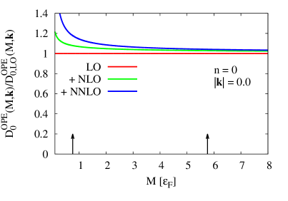
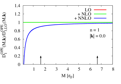
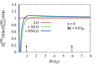
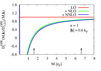
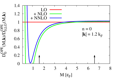
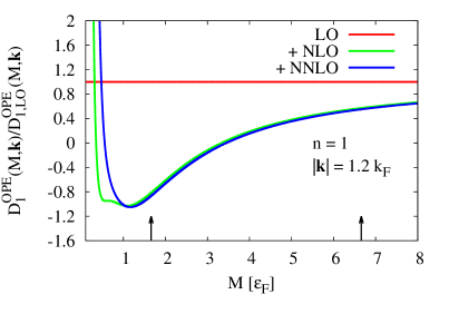
Figure 3: The right-hand sides of Eqs.(27) and (28), divided by their LO terms, as a function of the Borel mass $M$. The left and right plots show the cases of $n=0$ and $n=1$, respectively. Starting from the top, each line shows the OPE for momenta $|\bm{k}|/k_{\mathrm{F}}=0$, $0.6$ and $1.2$. Here, LO corresponds to the first line on the right-hand side of Eqs.(27) and (28), NLO to the second and third lines and NNLO to the fourth and fifth lines. The vertical arrows at the bottom of each plot indicate the lower and upper boundaries of the regions of $M$, which will be used in the MEM analysis of Section III.

The sum rules of Eqs.(27) and (28) look quite cumbersome, but their analytic structure becomes clearer if one takes the small momentum limit ($\epsilon_{\bm{k}}\to 0$). Using the kernel of Eq.(26) with general values of $n$, one can show that in this limit the LO term behaves as $M^{1/2+n}$ and the NNLO term as $M^{-1/2+n}$. The NLO term on the other hand can be shown to be proportional to $M^{0}=1$ for $n=0$, while it vanishes for all other positive $n$ values. The results for $n=0$ and $n=1$ are given by

$$\int^{\infty}_{-\infty}d\omega\mathcal{K}_{0}(\omega,M)\mathrm{Im}\Sigma_{\uparrow}(\omega,\bm{k})$$

$$= -\frac{2\sqrt{2}}{3\pi}\Gamma(1/4)\epsilon_{\mathrm{F}}^{3/2}M^{1/2}-\frac{0.207498}{3\pi}\epsilon_{\mathrm{F}}^{2}\zeta-\frac{4}{5}\frac{1}{\Gamma(1/4)}\epsilon_{\mathrm{F}}^{5/2}\Bigl{(}\xi-\frac{5}{3}\frac{\epsilon_{\bm{k}}}{\epsilon_{\mathrm{F}}}\Bigr{)}\frac{1}{M^{1/2}}$$ (30)

and

$$\int^{\infty}_{-\infty}d\omega\mathcal{K}_{1}(\omega,M)\mathrm{Im}\Sigma_{\uparrow}(\omega,\bm{k})$$

$$= -\frac{4}{3}\frac{1}{\Gamma(1/4)}\epsilon_{\mathrm{F}}^{3/2}M^{3/2}+\frac{\sqrt{2}}{10\pi}\Gamma(1/4)\epsilon_{\mathrm{F}}^{5/2}\Bigl{(}\xi-\frac{5}{3}\frac{\epsilon_{\bm{k}}}{\epsilon_{\mathrm{F}}}\Bigr{)}M^{1/2}.$$ (31)

Here, the term proportional to $\epsilon_{\bm{k}}$ in the last term comes from Taylor expanding the leading order terms of the first lines of Eqs.(27) and (28) in $\epsilon_{\bm{k}}/M$. The above equations should give the reader an idea on the behavior of the OPE at least for small $|\bm{k}|$. In the actual analysis of the next section, we will however use the full result of Eqs.(27) and (28).

III MEM analysis for the spectral density

Next, we discuss the imaginary parts of the self-energies, which we have extracted numerically from the sum rules by using the maximum entropy method (MEM). This sort of approach for analyzing sum rules, was recently applied to QCD in a similar way Gubler and has during the last few years been used to study hadrons in various environments Ohtani ; Gubler3 ; Gubler2 ; Suzuki ; Ohtani2 ; Gubler4 . For the technical details of this analysis, we refer the reader to Appendix D and the references cited therein.

III.1 The Borel window and the default model

Before discussing our results, let us here at first briefly explain how to determine the lower and upper boundaries of the Borel mass $M$ used in the analysis. For fixing the lower boundary $M_{\mathrm{min}}$, we demand that the highest order (NNLO) OPE term, which is proportional to $\xi$, should be smaller than 10% of the leading order term. Note, that this condition generally leads to a value of $M_{\mathrm{min}}$, which depends on the momentum $|\bm{k}|$. We will here first fix $M_{\mathrm{min}}$ at $|\bm{k}|=0$ and take this momentum dependence into account only if it leads to an increasing value of $M_{\mathrm{min}}$. This keeps the momentum dependence of $M_{\mathrm{min}}$ to a minimum and at the same time ensures that for any value of $|\bm{k}|$, only Borel mass ranges with a satisfactory OPE convergence are used as input for the MEM analysis.

For fixing the upper boundary $M_{\mathrm{max}}$, we do not have such a clear-cut criterion and therefore can in principle choose it freely as long as it lies above $M_{\mathrm{min}}$. For the analysis presented in this paper, we will set it as $M_{\mathrm{max}}=M_{\mathrm{min}}+x$, with $x=5\,\epsilon_{F}$. We have checked that our results do not much depend on this choice and the exact value of $x$ hence does not play any important role in the present analysis. The specific values of $M_{\mathrm{min}}$ and $M_{\mathrm{max}}$ for some typical momentum values are indicated in Fig. 3 as vertical arrows at the bottom of each plot.

As for the default model $m(\omega)$, which is an input of the MEM algorithm (see Appendix D for details), we will use

$$m(\omega)=-\frac{4\sqrt{2}}{3\pi}\epsilon_{\mathrm{F}}^{3/2}\frac{1}{(\omega^{2}+y)^{1/4}},$$ (32)

with $y=\epsilon_{\mathrm{F}}^{2}$. As can be understood from Eq.(21), the above default model approaches the correct asymptotic limit of $\mathrm{Im}\Sigma_{\uparrow}(\omega,\bm{k})\simeq-(4\sqrt{2}\epsilon_{\mathrm{F}}^{3/2})/(3\pi\sqrt{\omega})$, as $\omega\gg\epsilon_{\bm{k}}$ and is therefore a suitable choice for the present analysis. For avoiding singularities at $\omega=0$, we have introduced the parameter $y$ for smoothing out the function around the origin. We have tested different choices for $y$ and found that this affects our analysis results only very weakly.

III.2 The single-particle spectral density

After these preparations, we can now finally proceed to our analysis results. First, we show the imaginary part of the self-energy, for three representative momenta in the left column of Fig. 4.

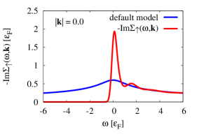
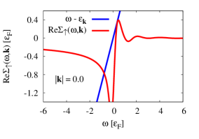
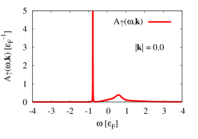
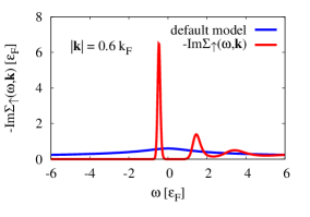
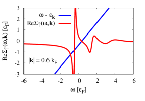
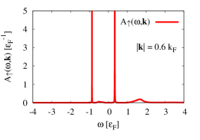
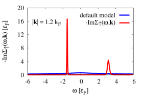
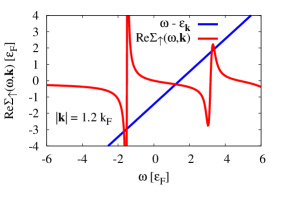
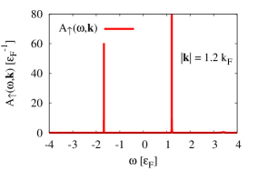
Figure 4: Left column: Results of the MEM analysis of Eqs.(27) and (28) are shown as red lines, while the used default model [see Eq.(32)] is indicated in blue. Middle column: The real parts of the self-energies obtained from Eq.(33) and $\mathrm{Im}\Sigma_{\uparrow}(\omega,{\bm{k}})$ are plotted as red lines, and the function $\omega-\epsilon_{\bm{k}}$ is given in blue. Right column: The spectral density $A_{\uparrow}(\omega,\bm{k})$, as computed from the results of the two columns on the left and Eq.(3). As in Fig. 3, each row from top to bottom corresponds to momenta $|\bm{k}|/k_{\mathrm{F}}=0.0$, $0.6$ and $1.2$, respectively.

For illustration, we show in these plots also the used default model of Eq.(32). It is seen that for zero momentum, the spectral function is composed of one single peak around $\omega=0$ and a continuum behaving as $\sim 1/\sqrt{\omega}$ in the positive energy region. As the momentum increases, the initial peak separates into two distinct peaks which start to move into opposite directions. The continuum also recedes into the positive $\omega$ region with increasing momentum, leaving a growing region around the origin without any strength at all.

With the extracted $\mathrm{Im}\Sigma_{\uparrow}(\omega,\bm{k})$, we next compute the real part of the self-energy by using the Kramers-Kr$\mathrm{\ddot{o}}$nig relation

$$\mathrm{Re}\Sigma_{\uparrow}(\omega,\bm{k})=-\frac{1}{\pi}\mathrm{P}\int_{-\infty}^{\infty}d\omega^{\prime}\frac{\mathrm{Im}\Sigma_{\uparrow}(\omega^{\prime},\bm{k})}{\omega-\omega^{\prime}},$$ (33)

and executing the principal value integral numerically. The result of this evaluation is given in the middle column of Fig. 4, where we also show the curve $\omega-\epsilon_{\bm{k}}$, which appears in the denominator of the right-hand side of Eq.(3). It is clear from this equation that if the imaginary part of the self-energy happens to be small, the single-particle spectral density will have a narrow peak wherever $\mathrm{Re}\Sigma_{\uparrow}(\omega,\bm{k})$ coincides with $\omega-\epsilon_{\bm{k}}$.

As a last step, we simply plug the real and imaginary parts of the self-energy into

$$A_{\uparrow}(\omega,\bm{k})=-\frac{1}{\pi}\mathrm{Im}\frac{1}{\omega+i0^{+}-\epsilon_{\bm{k}}-\Sigma_{\uparrow}(\omega+i0^{+},\bm{k})},$$ (34)

to obtain the single-particle spectral density $A_{\uparrow}(\omega,\bm{k})$. The resulting functions are given in the right column of Fig. 4. It can be seen there, that for small momenta $|\bm{k}|$, the spectral density is dominated by the narrow hole-branch in the negative energy region, while the particle-branch consists of only a relatively broad bump. This changes at around $|\bm{k}|\sim 0.5\,k_{\mathrm{F}}$, where the main strength of the spectral density switches over to the particle branch, which, as the momentum is further increased, starts to move into the positive energy direction. On the other hand, the hole-branch bends back into the negative energy region, while gradually losing its strength. To give the reader a better visual grasp of the spectral density as a whole and especially on the behavior of the particle and hole branches, we show $A_{\uparrow}(\omega,\bm{k})$ in a density plot as a function of both energy $\omega$ and momentum $|\bm{k}|$ in Fig. 5. To improve the visibility of this plot without changing its essential features, we have artificially increased the imaginary part of $\Sigma_{\uparrow}(\omega,\bm{k})$ in Eq.(34) by an amount of $0.2\,\epsilon_{\mathrm{F}}$.

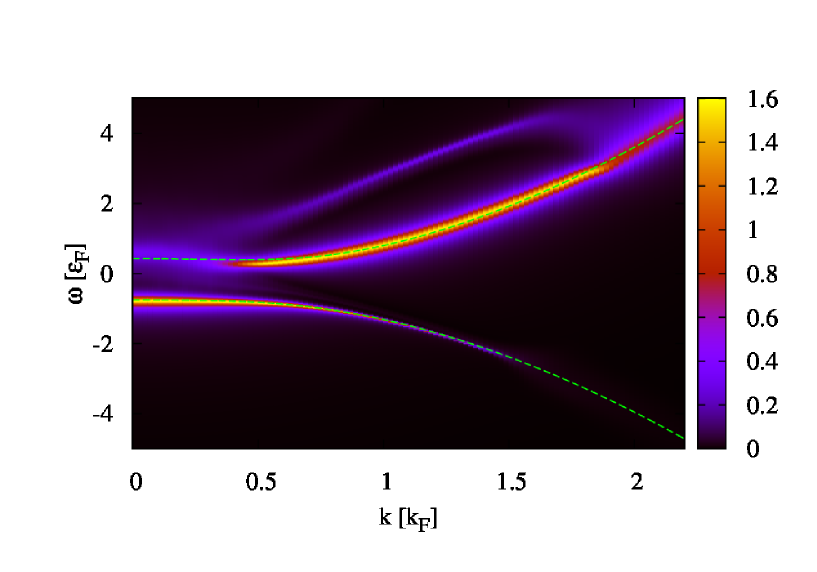
Figure 5: Density plot of the spectral density $A_{\uparrow}(\omega,\bm{k})$ shown as a function of energy $\omega$ and momentum $|\bm{k}|$. The green dashed lines indicate the results of a fit of the particle and hole peak-maxima to Eq.(35).

In this figure, the typical BCS-like dispersion of the particle and hole branches clearly manifest themselves. Qualitatively, this result agrees with the spectral densities extracted from both quantum Monte-Carlo calculations Magierski and a Luttinger-Ward approach Haussmann . In order to make a quantitative comparison with other methods, we fit the peak maxima to a dispersion relation parametrized as

$$E_{\bm{k}}^{\pm}=\mu\pm\sqrt{\left(\frac{m}{m^{\pm}}\epsilon_{\bm{k}}+U^{\pm}-\mu\right)^{2}+\Delta^{2}},$$ (35)

which we have adopted from Haussmann . The resultant curves are shown in Fig. 5 as green dashed lines, while the corresponding values of $\mu$, $\Delta$, $m^{\pm}$ and $U^{\pm}$ are given in Table 2.

Table 2: Fit results of the particle and hole branches shown in Fig. 5 to a dispersion relation parametrized as in Eq.(35).

			Particle		Hole
	$\mu/\epsilon_{\mathrm{F}}$	$\Delta/\epsilon_{\mathrm{F}}$	$m^{+}/m$	$U^{+}/\epsilon_{\mathrm{F}}$	$m^{-}/m$	$U^{-}/\epsilon_{\mathrm{F}}$
this work	-0.18	0.57	1.02	-0.37	1.09	-0.12
Haussmann	0.36	0.46	1.00	-0.50	1.19	-0.35

It is seen in Figure 5 that the fit is able to reproduce our dispersion relation fairly well, with the exception of the low momentum region of the particle branch, whose curvature can not be captured fully by the simple formula of Eq.(35). Note that this leads to a slight overestimation of the gap $\Delta$. If we simply read it of from the point at which the particle and hole branches are closest, we get a value of $\Delta/\epsilon_{\mathrm{F}}=0.54$ instead of the one given in Table 2.

Comparing the values of this work with those of Haussmann , it is seen that the two approaches give comparable results for the gap parameter $\Delta$, effective masses $m^{\pm}$ and Hartree shifts $U^{\pm}$ for both the particle and hole branches. On the other hand, the chemical potential $\mu$ deviates significantly from Haussmann , even giving a different sign. The reason for this discrepancy apparently originates in the low sensitivity of the sum rules to the absolute position of the $\omega$ axis. This can be understood by inspecting the OPE of Eq.(21). After setting $k_{0}=\omega$ and making a change of variables $\omega\to\omega^{\prime}$ as $\omega=\omega^{\prime}+\omega_{0}$, with $\omega_{0}$ of the order of $\epsilon_{\mathrm{F}}$ and expanding the resulting expression in $\omega_{0}/\omega^{\prime}$, one notes that only the NNLO term of the OPE will be modified, which must be kept small due to the convergence condition of the OPE. Therefore, we can expect that such a change of variables will introduce no qualitative modification of the OPE, while the spectral density experiences a parallel shift of $\omega_{0}$.

It is in principle possible to choose $\omega_{0}$ such that the fitted value of $\mu$ approaches the correct value of around $0.36\,\epsilon_{\mathrm{F}}$. Due to the convergence criterion of the OPE, such a choice however leads to a significantly larger value of $M_{\mathrm{min}}$ and therefore to a rather poor resolution of the MEM extraction of $\mathrm{Im}\Sigma_{\uparrow}(\omega,\bm{k})$. We have thus not explored this possibility any further and simply note that at the present stage, the absolute positions of the structures appearing in the spectral density should not be taken too seriously.

As a final point, we study the density of states of the single argument $\omega$, $\rho_{\uparrow}(\omega)$, which is obtained by integrating the spectral density over the momentum $|\bm{k}|$:

$$\rho_{\uparrow}(\omega)=\int\frac{d^{3}k}{(2\pi)^{3}}A_{\uparrow}(\omega,\bm{k}).$$ (36)

This function is shown in Fig. 6, from which one can immediately read off the approximate gap value, which can be regarded as half the width of the region where $\rho_{\uparrow}(\omega)$ loses almost all of its strength. To draw Fig. 6, we have added an constant amount of $0.002\,\epsilon_{\mathrm{F}}$ to the imaginary part of $\Sigma_{\uparrow}(\omega,\bm{k})$, which reduces artificial effects caused by evaluating the integral numerically from a discrete number of data points, but does not change the gap structure of this plot.

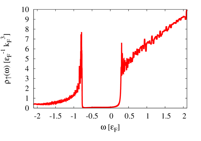
Figure 6: The density of states, $\rho_{\uparrow}(\omega)$, obtained by integrating the spectral density $A_{\uparrow}(\omega,\bm{k})$ over the momentum $\bm{k}$ as shown in Eq.(36).

IV Summary and conclusion

The work presented in this paper was carried out with two essential goals in mind. As the introduced techniques are new and have not been applied to cold atom systems so far, we first needed to test to what extent the sum rules and MEM are able to extract the single-particle spectral density from the result of the OPE. This is by no means a trivial test, because the OPE considered in momentum space does not converge for momenta below the Fermi momentum Nishida , as we have already discussed in the introduction. It was therefore at the beginning not clear to what degree the sum rules can extend the applicability of the OPE to lower momenta or energies. As it however turns out, even at zero momentum $|\bm{k}|$ and small $\omega$, the sum rules of Eqs.(27) and (28) lead a fairly reasonable behavior for the spectral density, which suggests that our approach is indeed useful for extracting the spectral density at any momentum and energy.

Once the proposed method is proven to work well, our second goal was to provide an independent framework for evaluating the superfluid pairing gap $\Delta$ of the unitary Fermi gas. Our obtained value is given in Table 2 and can be inferred from Fig. 5. We wish to emphasize here that even though we have only taken into account the first few terms of the OPE, in which the Bertsch parameter and the contact density are the only input values, our numerical result shows reasonable agreement with other theoretical approaches Haussmann ; Carlson2 . Specifically, we obtain $\Delta/\epsilon_{\mathrm{F}}=0.54$, when extracting the gap from point of smallest distance between the particle and hole branches and $\Delta/\epsilon_{\mathrm{F}}=0.57$ from an overall fit of our dispersion relation to Eq.(35), while Haussmann and Carlson2 get $\Delta/\epsilon_{\mathrm{F}}=0.46$ and $\Delta/\epsilon_{\mathrm{F}}=0.50(3)$, respectively. For confirming these results in the future, it will be necessary to consider still higher order terms in the OPE, evaluate the size of their contributions and examine their impact on the spectral density.

Using the method proposed in this work, we have so far only studied the fermionic single-particle channel at zero temperature. As long as the conditions for its applicability (that is $r_{0}\ll 1/\sqrt{|k_{0}|}\ll|a|,\,n^{-1/3},\,\lambda_{T}$) are satisfied, the OPE technique is fairly general and can in principle be applied to any kind of bosonic or fermionic systems with one or more constituents. One can therefore envisage various future applications of this approach. For instance, in Goldberger the OPE for the retarded correlator of the density operator has already been worked out, and one in principle just needs to apply MEM or some other sort of fitting method to extract information on the dynamic structure factor from the OPE expression. Another interesting direction of research could be the generalization of this approach to finite temperature. For being able to do this, one however needs information on the finite temperature behavior of the operator expectation values which appear in the OPE of the channel of interest. For the system considered in this paper, this would correspond to the finite temperature values of the Bertsch parameter and the contact density, which are calculable using quantum Monte-Carlo simulations Drut .

Appendix A Numerical solution of $T^{\mathrm{reg}}_{\uparrow}(k,0;k,0)$ in the unitary limit

As discussed in Section II.2, we need to solve the integral equation given in Eq.(15) numerically, which is then substituted in Eq.(17) to obtain the desired scattering amplitude $T^{\mathrm{reg}}_{\uparrow}(k,0;k,0)$. The technical details necessary for this task will be outlined in this Appendix, in which we generalize the discussion given in Appendix B of Nishida , where $k_{0}$ was set to $\epsilon_{\bm{k}}$, while we here have to keep it as an independent variable and will specifically consider $k_{0}=\omega+i0^{+}$, with $\omega$ being real.

Firstly, it is noticed that the dimensionless function

$$s_{\uparrow}(k;\epsilon_{\bm{p}},{\bm{p}})=\frac{{\bm{k}}^{2}}{m}T_{\uparrow}(k;\epsilon_{\bm{p}},{\bm{p}}+\tfrac{1}{3}{\bm{k}})$$ (37)

satisfies a simpler integral equation, which is given as

$$\begin{split}s_{\uparrow}(k;\epsilon_{\bm{p}},{\bm{p}})=&-\frac{{\bm{k}}^{2}}{({\bm{p}}+\tfrac{1}{3}{\bm{k}})^{2}}\\ &-\int\!\frac{d{\bm{q}}}{(2\pi)^{3}}\frac{16\pi}{\sqrt{3{\bm{q}}^{2}+\tfrac{2}{3}{\bm{k}}^{2}-4mk_{0}}}\frac{s_{\uparrow}(k;\epsilon_{\bm{q}},{\bm{q}})}{2{\bm{p}}^{2}+2{\bm{q}}^{2}+2{\bm{p}}\cdot{\bm{q}}+\tfrac{1}{3}{\bm{k}}^{2}-2mk_{0}}\\ \equiv&-\mathcal{I}({\bm{k}};{\bm{p}})-\int\!\frac{d{\bm{q}}}{(2\pi)^{3}}\mathcal{J}(k;{\bm{p}},{\bm{q}})s_{\uparrow}(k;\epsilon_{\bm{q}},{\bm{q}}).\end{split}$$ (38)

The important point here is that the Kernel $\mathcal{J}(k;{\bm{p}},{\bm{q}})$ now depends only on the angle between ${\bm{q}}$ and ${\bm{p}}$, which will permit a partial wave expansion of the above integral equation.

Next, we expand $s_{\uparrow}(k;\epsilon_{\bm{p}},{\bm{p}})$ into its partial waves, which depend on the angle $\theta$ between ${\bm{k}}$ and ${\bm{p}}$ as

$$s_{\uparrow}(k;\epsilon_{\bm{p}},{\bm{p}})=\sum_{l=0}^{\infty}s_{\uparrow}^{(l)}\Big{(}\tfrac{k_{0}}{\epsilon_{\bm{k}}},\tfrac{\epsilon_{\bm{p}}}{\epsilon_{\bm{k}}}\Big{)}P_{l}(\cos\theta),$$ (39)

where $P_{l}(x)$ are the Legendre polynomials. We have made use of the fact that $s_{\uparrow}^{(l)}$ is a dimensionless function, which can hence only depend on the ratios $k_{0}/\epsilon_{\bm{k}}$ and $\epsilon_{\bm{p}}/\epsilon_{\bm{k}}$. It can be shown that each term $s_{\uparrow}^{(l)}(k_{0}/\epsilon_{\bm{k}},\epsilon_{\bm{p}}/\epsilon_{\bm{k}})$ in the sum of Eq.(39) satisfies a closed integral equation,

$$s_{\uparrow}^{(l)}\Big{(}\tfrac{k_{0}}{\epsilon_{\bm{k}}},\tfrac{\epsilon_{\bm{p}}}{\epsilon_{\bm{k}}}\Big{)}=-\mathcal{I}^{(l)}\Big{(}\tfrac{\epsilon_{\bm{p}}}{\epsilon_{\bm{k}}}\Big{)}-\int_{0}^{\infty}d\tfrac{|{\bm{q}}|}{|{\bm{k}}|}\mathcal{J}^{(l)}\Big{(}\tfrac{k_{0}}{\epsilon_{\bm{k}}},\tfrac{\epsilon_{\bm{p}}}{\epsilon_{\bm{k}}},\tfrac{\epsilon_{\bm{q}}}{\epsilon_{\bm{k}}}\Big{)}s_{\uparrow}^{(l)}\Big{(}\tfrac{k_{0}}{\epsilon_{\bm{k}}},\tfrac{\epsilon_{\bm{q}}}{\epsilon_{\bm{k}}}\Big{)}.$$ (40)

Here, the function $\mathcal{I}^{(l)}$ is defined as

$$\mathcal{I}^{(l)}\Big{(}\tfrac{\epsilon_{\bm{p}}}{\epsilon_{\bm{k}}}\Big{)}\equiv\frac{2l+1}{2}\int_{-1}^{1}d\cos\theta P_{l}(\cos\theta)\mathcal{I}({\bm{k}};{\bm{p}}),$$ (41)

which can be rewritten with the help of the Gaussian hypergeometric function ${}_{2}F_{1}(a,b;c;y)$:

$$\mathcal{I}^{(l)}(x)=\frac{l!}{(2l-1)!!}\frac{9}{1+9x}\Big{(}-\frac{6\sqrt{x}}{1+9x}\Big{)}^{l}\,_{2}F_{1}\Bigg{[}\frac{l+1}{2},\frac{l+2}{2};l+\frac{3}{2};\frac{36x}{(1+9x)^{2}}\Bigg{]}.$$ (42)

Furthermore, we have defined $\mathcal{J}^{(l)}$ as shown below:

$$\mathcal{J}^{(l)}\Big{(}\tfrac{k_{0}}{\epsilon_{\bm{k}}},\tfrac{\epsilon_{\bm{p}}}{\epsilon_{\bm{k}}},\tfrac{\epsilon_{\bm{q}}}{\epsilon_{\bm{k}}}\Big{)}\equiv\frac{|{\bm{k}}||{\bm{q}}|^{2}}{4\pi^{2}}\int_{-1}^{1}d\cos\theta P_{l}(\cos\theta)\mathcal{J}(k;{\bm{p}},{\bm{q}}).$$ (43)

Using again the Gaussian hypergeometric function this gives,

$$\begin{split}\mathcal{J}^{(l)}(x,y,z)=&\>\frac{8}{\pi}\frac{l!}{(2l+1)!!}\frac{z}{\sqrt{3z+\tfrac{2}{3}-2x}}\frac{1}{2y+2z+\tfrac{1}{3}-x}\Big{(}\frac{2\sqrt{yz}}{2y+2z+\tfrac{1}{3}-x}\Big{)}^{l}\\ &\times_{2}F_{1}\Bigg{[}\frac{l+1}{2},\frac{l+2}{2};l+\frac{3}{2};\frac{4yz}{(2y+2z+\tfrac{1}{3}-x)^{2}}\Bigg{]}.\end{split}$$ (44)

As a next step, we need to solve Eq.(40) numerically for general values of $l$. In practice, we however will not deal with this equation directly, but first define

$$\delta s_{\uparrow}^{(l)}\Big{(}\tfrac{k_{0}}{\epsilon_{\bm{k}}},\tfrac{\epsilon_{\bm{p}}}{\epsilon_{\bm{k}}}\Big{)}=s_{\uparrow}^{(l)}\Big{(}\tfrac{k_{0}}{\epsilon_{\bm{k}}},\tfrac{\epsilon_{\bm{p}}}{\epsilon_{\bm{k}}}\Big{)}+\mathcal{I}^{(l)}\Big{(}\tfrac{\epsilon_{\bm{p}}}{\epsilon_{\bm{k}}}\Big{)},$$ (45)

which satisfies

$$\begin{split}\delta s_{\uparrow}^{(l)}\Big{(}\tfrac{k_{0}}{\epsilon_{\bm{k}}},\tfrac{\epsilon_{\bm{p}}}{\epsilon_{\bm{k}}}\Big{)}=&\int_{0}^{\infty}d\tfrac{|{\bm{q}}|}{|{\bm{k}}|}\mathcal{J}^{(l)}\Big{(}\tfrac{k_{0}}{\epsilon_{\bm{k}}},\tfrac{\epsilon_{\bm{p}}}{\epsilon_{\bm{k}}},\tfrac{\epsilon_{\bm{q}}}{\epsilon_{\bm{k}}}\Big{)}\mathcal{I}^{(l)}\Big{(}\tfrac{\epsilon_{\bm{q}}}{\epsilon_{\bm{k}}}\Big{)}\\ &-\int_{0}^{\infty}d\tfrac{|{\bm{q}}|}{|{\bm{k}}|}\mathcal{J}^{(l)}\Big{(}\tfrac{k_{0}}{\epsilon_{\bm{k}}},\tfrac{\epsilon_{\bm{p}}}{\epsilon_{\bm{k}}},\tfrac{\epsilon_{\bm{q}}}{\epsilon_{\bm{k}}}\Big{)}\delta s_{\uparrow}^{(l)}\Big{(}\tfrac{k_{0}}{\epsilon_{\bm{k}}},\tfrac{\epsilon_{\bm{q}}}{\epsilon_{\bm{k}}}\Big{)},\end{split}$$ (46)

and then solve this equation for $\delta s_{\uparrow}^{(l)}(k_{0}/\epsilon_{\bm{k}},\epsilon_{\bm{p}}/\epsilon_{\bm{k}})$. This is done in order to avoid (or at least to weaken) the singularities that appear in $s_{\uparrow}^{(l)}(k_{0}/\epsilon_{\bm{k}},\epsilon_{\bm{p}}/\epsilon_{\bm{k}})$ for certain values of $k_{0}/\epsilon_{\bm{k}}$ and $\epsilon_{\bm{p}}/\epsilon_{\bm{k}}$ and use instead the better behaved $\delta s_{\uparrow}^{(l)}(k_{0}/\epsilon_{\bm{k}},\epsilon_{\bm{p}}/\epsilon_{\bm{k}})$. Once this is done, the result is substituted into Eq.(22), which, by making use of the above definitions, can be rephrased as

$$\begin{split}L\Big{(}\frac{k_{0}}{\epsilon_{\bm{k}}}\Big{)}=&\>\epsilon_{\bm{k}}\int\!\frac{d{\bm{q}}}{(2\pi)^{3}}\frac{8\pi}{\sqrt{3{\bm{q}}^{2}-2{\bm{q}}\cdot{\bm{k}}+{\bm{k}}^{2}-4mk_{0}}}\frac{T_{\uparrow}(k;\epsilon_{\bm{q}},{\bm{q}})+\frac{m}{{\bm{q}}^{2}}}{{\bm{q}}^{2}}\\ =&\>\frac{\sqrt{2}}{\pi}\sum_{l=0}^{\infty}\frac{1}{2l+1}\int_{0}^{\infty}d\tfrac{|{\bm{q}}|}{|{\bm{k}}|}\frac{\tfrac{\epsilon_{\bm{q}}}{\epsilon_{\bm{k}}}}{\sqrt{\tfrac{3}{2}\tfrac{\epsilon_{\bm{q}}}{\epsilon_{\bm{k}}}+\tfrac{1}{3}-\tfrac{k_{0}}{\epsilon_{\bm{k}}}}}\mathcal{I}^{(l)}\Big{(}\tfrac{\epsilon_{\bm{q}}}{\epsilon_{\bm{k}}}\Big{)}\delta s_{\uparrow}^{(l)}\Big{(}\tfrac{k_{0}}{\epsilon_{\bm{k}}},\tfrac{\epsilon_{\bm{q}}}{\epsilon_{\bm{k}}}\Big{)}.\end{split}$$ (47)

After obtaining $\delta s_{\uparrow}^{(l)}(k_{0}/\epsilon_{\bm{k}},\epsilon_{\bm{p}}/\epsilon_{\bm{k}})$ for each value of $l$ individually, the corresponding contributions are added in Eq.(47), which then gives the final form of $L(k_{0}/\epsilon_{\bm{k}})$. It suffices to evaluate the function $L(k_{0}/\epsilon_{\bm{k}})$ for one specific value of $\epsilon_{\bm{k}}$, as its form for general $\epsilon_{\bm{k}}$ can be obtained by a simple rescaling of its argument.

In Fig. 7, we show the final results for $\mathrm{Im}\bigl{[}L(x)\bigr{]}$ for various maximum values of $l$ in the sum of Eq.(47). (We show only the imaginary part because this is the only piece that will be needed for constructing the sum rules.)

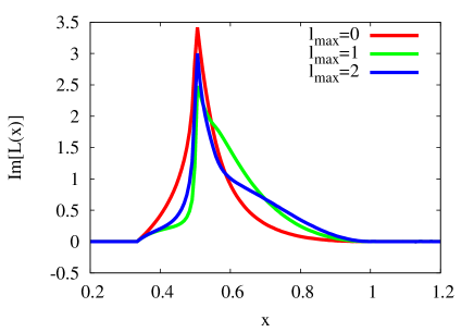
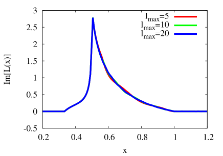
Figure 7: $\mathrm{Im}\bigl{[}L(x)\bigr{]}$, obtained by solving Eq.(46) and adding up the results in Eq.(47) to various maximum values of $l$.

It is seen in these plots that $\mathrm{Im}\bigl{[}L(x)\bigr{]}$ is essentially determined by the first 5 terms in the sum over $l$ and that the expansion converges quickly for values beyond $l\sim 10$. In this work, we will take into account the terms up to $l=20$.

Furthermore, it can be seen in Fig. 7 that $\mathrm{Im}\bigl{[}L(x)\bigr{]}$ takes non-zero values only in the interval $\tfrac{1}{3}<x<1$, where it peaks sharply at around $x\sim 0.5$.

Appendix B Derivation of the sum rules for a generic kernel

To derive the general form of the sum rule, given in Eq.(25), we need to compute the right-hand side of Eq.(24), or, to be more precise, need to evaluate the contour integrals of $\mathcal{K}(k_{0})\Sigma^{\mathrm{OPE}}(k_{0},{\bm{k}})$ along the sections of the contours $C_{1}$ and $C_{2}$, which run above and below the real axis. The OPE expression for the self-energy is given in Eq.(21) of Section II.4 and is reproduced here once more:

$$\begin{split}&\Sigma^{\mathrm{OPE}}_{\uparrow}(k_{0},\bm{k})=\\ &-\frac{8}{3\pi}\epsilon_{\mathrm{F}}^{3/2}\frac{1}{\sqrt{\epsilon_{\bm{k}}-2k_{0}}}+\frac{4}{3\pi^{2}}\zeta\epsilon_{\mathrm{F}}^{2}\Biggl{[}\frac{1}{k_{0}+\epsilon_{\bm{k}}}-\frac{\sqrt{3}}{\pi}\frac{1}{2k_{0}-\epsilon_{\bm{k}}}\\ &-\frac{1}{\pi}\frac{3k_{0}-\epsilon_{\bm{k}}}{\sqrt{\epsilon_{\bm{k}}}(\epsilon_{\bm{k}}-2k_{0})^{3/2}}\log\Bigg{(}\frac{1+\sqrt{3}\sqrt{1-2k_{0}/\epsilon_{\bm{k}}}}{-1+\sqrt{3}\sqrt{1-2k_{0}/\epsilon_{\bm{k}}}}\Bigg{)}+\frac{1}{\epsilon_{\bm{k}}}L\bigl{(}\tfrac{k_{0}}{\epsilon_{\bm{k}}}\bigr{)}\Biggr{]}\\ &-\frac{8}{5\pi}\xi\epsilon_{\mathrm{F}}^{5/2}\frac{\epsilon_{\bm{k}}-k_{0}}{(\epsilon_{\bm{k}}-2k_{0})^{5/2}}+O(k_{0}^{-2}).\end{split}$$ (48)

The kernel $\mathcal{K}(k_{0})$ is assumed to be analytic in the whole complex $k_{0}$ plane and to vanish faster that $1/\sqrt{k_{0}}$ at $k_{0}\to\infty$ on the positive real axis.

As some of the derivations are somewhat involved, we will consider each term of the OPE individually. As in the main text, we here consider $k_{0}$ to be a complex variable, while $\omega$ is understood to be purely real.

B.1 Leading order (LO)

Using

$$\mathrm{Im}\Bigl{[}\frac{1}{\sqrt{\epsilon_{\bm{k}}-2\omega-i0^{+}}}\Bigr{]}=\theta(2\omega-\epsilon_{\bm{k}})\frac{1}{\sqrt{2\omega-\epsilon_{\bm{k}}}},$$ (49)

we immediately get,

$$\begin{split}&\int^{\infty}_{-\infty}d\omega\mathcal{K}(\omega)\mathrm{Im}\Sigma^{\mathrm{LO}}_{\uparrow}(\omega+i0^{+},{\bm{k}})\\ &=-\frac{8}{3\pi}\epsilon_{\mathrm{F}}^{3/2}\int^{\infty}_{\epsilon_{\bm{k}}/2}d\omega\frac{1}{\sqrt{2\omega-\epsilon_{\bm{k}}}}\mathcal{K}(\omega)\\ &=\frac{8}{3\pi}\epsilon_{\mathrm{F}}^{3/2}\int^{\infty}_{\epsilon_{\bm{k}}/2}d\omega\sqrt{2\omega-\epsilon_{\bm{k}}}\mathcal{K}^{\prime}(\omega).\end{split}$$ (50)

Note that for the above integrals to converge, the assumption of $\mathcal{K}(\omega)$ to approach 0 quicker than $1/\sqrt{\omega}$ at $\omega\to\infty$ is needed here.

B.2 Next-to-leading order (NLO)

Being proportional to the contact density parameter $\zeta$, the NLO expression consists of two pole terms, one $\log$-term and one term containing the function $L(k_{0}/\epsilon_{\bm{k}})$. The pole terms are easily treated using

$$\mathrm{Im}\Bigl{[}\frac{1}{\omega-x+i0^{+}}\Bigr{]}=-\pi\delta(\omega-x),$$ (51)

which gives

$$\begin{split}&\int^{\infty}_{-\infty}d\omega\mathcal{K}(\omega)\mathrm{Im}\Sigma^{\mathrm{NLO,\,\mathrm{pole}}}_{\uparrow}(\omega+i0^{+},{\bm{k}})\\ &=-\frac{4}{3\pi}\zeta\epsilon_{\mathrm{F}}^{2}\Bigl{[}\mathcal{K}(-\epsilon_{\bm{k}})-\frac{\sqrt{3}}{2\pi}\mathcal{K}\big{(}\tfrac{\epsilon_{\bm{k}}}{2}\big{)}\Bigr{]}.\end{split}$$ (52)

Next, we consider the $\log$-term, which needs a somewhat more careful treatment of the contour integral, because simply taking its imaginary part leads to a divergence at $\omega=\epsilon_{\bm{k}}/2$. Before doing this, we note that

$$\frac{1+\sqrt{3}\sqrt{1-2\omega/\epsilon_{\bm{k}}}}{-1+\sqrt{3}\sqrt{1-2\omega/\epsilon_{\bm{k}}}},$$ (53)

which is the argument of the $\log$ in Eq.(21), is positive and real for $\omega<\epsilon_{\bm{k}}/3$ and negative and real for $\epsilon_{\bm{k}}/3<\omega<\epsilon_{\bm{k}}/2$, where the $\log$ therefore has a cut. On the other hand, for $\omega>\epsilon_{\bm{k}}/2$, the above expression can be rewritten as follows:

$$\begin{split}\frac{1+\sqrt{3}\sqrt{1-2\omega/\epsilon_{\bm{k}}-i0^{+}}}{-1+\sqrt{3}\sqrt{1-2\omega/\epsilon_{\bm{k}}-i0^{+}}}=&\>\frac{1-i\sqrt{3}\sqrt{2\omega/\epsilon_{\bm{k}}-1}}{-1-i\sqrt{3}\sqrt{2\omega/\epsilon_{\bm{k}}-1}}\\ =&\>\frac{1}{3\omega-\epsilon_{\bm{k}}}\Bigl{(}3\omega-2\epsilon_{\bm{k}}-i\sqrt{3\epsilon_{\bm{k}}}\sqrt{2\omega-\epsilon_{\bm{k}}}\Bigr{)}\\ =&\>e^{i\theta},\end{split}$$ (54)

where $\theta$ is given as

$$\theta=\tan^{-1}\Bigl{(}\frac{\sqrt{3\epsilon_{\bm{k}}}\sqrt{2\omega-\epsilon_{\bm{k}}}}{3\omega-2\epsilon_{\bm{k}}}\Bigr{)}.$$ (55)

Therefore, the $\log$ of Eq.(53) is purely imaginary for $\omega>\epsilon_{\bm{k}}/2$. In this region, the root in front of the $\log$ in Eq.(21) is also purely imaginary, which means that the term as a whole is real and that there is no cut for $\omega>\epsilon_{\bm{k}}/2$.

Hence, it is understood that we just have to evaluate the contour shown in Fig. 8.

Figure 8: The contour integral on the complex plane of the variable $k_{0}$ needed to calculate the NLO $\log$-term contribution to the sum rule.

The corresponding analytical formula is

$$\begin{split}&\frac{1}{2i}\oint_{C_{1}\mathrm{-}C_{4}}dk_{0}\mathcal{K}(k_{0})\Sigma^{\mathrm{NLO,\,\mathrm{log}}}_{\uparrow}(k_{0},{\bm{k}})\\ &=-\frac{4}{3\pi^{3}}\zeta\frac{\epsilon_{\mathrm{F}}^{2}}{\sqrt{\epsilon_{\bm{k}}}}\frac{1}{2i}\oint_{C_{1}\mathrm{-}C_{4}}dk_{0}\mathcal{K}(k_{0})\frac{3k_{0}-\epsilon_{\bm{k}}}{(\epsilon_{\bm{k}}-2k_{0})^{3/2}}\log\Biggl{(}\frac{1+\sqrt{3}\sqrt{1-2k_{0}/\epsilon_{\bm{k}}}}{-1+\sqrt{3}\sqrt{1-2k_{0}/\epsilon_{\bm{k}}}}\Biggr{)},\end{split}$$ (56)

for which we below calculate the parts $C_{1}$ - $C_{4}$ separately.

Firstly, it is seen that the integrand is not singular at $k_{0}=\epsilon_{\bm{k}}/3$. Thus, the contour $C_{1}$ circling around this point vanishes as its radius approaches zero:

$$\begin{split}&\frac{1}{2i}\oint_{C_{1}}dk_{0}\mathcal{K}(k_{0})\Sigma^{\mathrm{NLO,\,\mathrm{log}}}_{\uparrow}(k_{0},{\bm{k}})=0.\end{split}$$ (57)

Next, the contour segments $C_{2}$ and $C_{4}$ are considered. They have a finite value due to the cut of the $\log$, which can be evaluated as follows:

$$\begin{split}&\frac{1}{2i}\oint_{C_{2}+C_{4}}dk_{0}\mathcal{K}(k_{0})\Sigma^{\mathrm{NLO,\,\mathrm{log}}}_{\uparrow}(k_{0},{\bm{k}})\\ =&-\frac{4}{3\pi^{2}}\zeta\frac{\epsilon_{\mathrm{F}}^{2}}{\sqrt{\epsilon_{\bm{k}}}}\int_{\epsilon_{\bm{k}}/3}^{\epsilon_{\bm{k}}/2-\epsilon}d\omega\mathcal{K}(\omega)\frac{3\omega-y^{2}}{(y^{2}-2\omega)^{3/2}}\\ =&-\frac{4}{3\pi^{2}}\zeta\epsilon_{\mathrm{F}}^{2}\Biggl{\{}\frac{\sqrt{\epsilon_{\bm{k}}}}{2\sqrt{2}}\mathcal{K}\bigl{(}\tfrac{\epsilon_{\bm{k}}}{2}\bigr{)}\frac{1}{\sqrt{\epsilon}}-\sqrt{3}\mathcal{K}\bigl{(}\tfrac{\epsilon_{\bm{k}}}{3}\bigr{)}\\ &-\frac{1}{\sqrt{\epsilon_{\bm{k}}}}\int_{\epsilon_{\bm{k}}/3}^{\epsilon_{\bm{k}}/2}d\omega\sqrt{\epsilon_{\bm{k}}-2\omega}\Bigl{[}6\mathcal{K}^{\prime}(\omega)-(\epsilon_{\bm{k}}-3\omega)\mathcal{K}^{\prime\prime}(\omega)\Bigr{]}\Biggr{\}}.\end{split}$$ (58)

Here, $\epsilon$ stands for the radius of the circle around $k_{0}=\epsilon_{\bm{k}}/2$ of the contour $C_{3}$. The last contribution comes from $C_{3}$, which, after a change of variables from $k_{0}$ to $\theta$ ($k_{0}=\epsilon_{\bm{k}}/2+\epsilon e^{i\theta}$), is divided into two parts:

$$\begin{split}&\>\frac{1}{2i}\oint_{C_{3}}d\omega\mathcal{K}(k_{0})\Sigma^{\mathrm{NLO,\,\mathrm{log}}}_{\uparrow}(k_{0},{\bm{k}})\\ =&\>\frac{\epsilon}{2}\int_{\pi}^{0}d\theta e^{i\theta}\mathcal{K}(\epsilon_{\bm{k}}/2+\epsilon e^{i\theta})\Sigma^{\mathrm{NLO,\,\mathrm{log}}}_{\uparrow}(\epsilon_{\bm{k}}/2+\epsilon e^{i\theta},{\bm{k}})\\ &+\frac{\epsilon}{2}\int_{0}^{-\pi}d\theta e^{i\theta}\mathcal{K}(\epsilon_{\bm{k}}/2+\epsilon e^{i\theta})\Sigma^{\mathrm{NLO,\,\mathrm{log}}}_{\uparrow}(\epsilon_{\bm{k}}/2+\epsilon e^{i\theta},{\bm{k}}).\end{split}$$ (59)

The first part is evaluated as

$$\begin{split}&\frac{\epsilon}{2}\int_{\pi}^{0}d\theta e^{i\theta}\mathcal{K}(\epsilon_{\bm{k}}/2+\epsilon e^{i\theta})\Sigma^{\mathrm{NLO,\,\mathrm{log}}}_{\uparrow}(\epsilon_{\bm{k}}/2+\epsilon e^{i\theta},{\bm{k}})\\ =&-\frac{2}{3\pi^{3}}\zeta\frac{\epsilon_{\mathrm{F}}^{2}}{\sqrt{\epsilon_{\bm{k}}}}\epsilon\int_{\pi}^{0}d\theta e^{i\theta}\mathcal{K}(\epsilon_{\bm{k}}/2+\epsilon e^{i\theta})\frac{3\bigl{(}\epsilon_{\bm{k}}/2+\epsilon e^{i\theta}\bigr{)}-\epsilon_{\bm{k}}}{\bigl{[}2\epsilon e^{i(\theta-\pi)}\bigr{]}^{3/2}}\\ &\times\log\Biggl{(}\frac{\sqrt{\epsilon_{\bm{k}}}+\sqrt{3}\sqrt{2\epsilon e^{i(\theta-\pi)}}}{-\sqrt{\epsilon_{\bm{k}}}+\sqrt{3}\sqrt{2\epsilon e^{i(\theta-\pi)}}}\Biggr{)}\\ =&\>\frac{\sqrt{2}}{6\pi^{2}}\zeta\epsilon_{\mathrm{F}}^{2}\sqrt{\epsilon_{\bm{k}}}\mathcal{K}\bigl{(}\tfrac{\epsilon_{\bm{k}}}{2}\bigr{)}(1-i)\frac{1}{\sqrt{\epsilon}}-\frac{1}{\sqrt{3}\pi^{2}}\zeta\epsilon_{\mathrm{F}}^{2}\mathcal{K}\bigl{(}\tfrac{\epsilon_{\bm{k}}}{2}\bigr{)},\end{split}$$ (60)

while the second one gives

$$\begin{split}&\frac{\epsilon}{2}\int_{0}^{-\pi}d\theta e^{i\theta}\mathcal{K}(\epsilon_{\bm{k}}/2+\epsilon e^{i\theta})\Sigma^{\mathrm{NLO,\,\mathrm{log}}}_{\uparrow}(\epsilon_{\bm{k}}/2+\epsilon e^{i\theta},{\bm{k}})\\ =&-\frac{2}{3\pi^{3}}\zeta\frac{\epsilon_{\mathrm{F}}^{2}}{\sqrt{\epsilon_{\bm{k}}}}\epsilon\int_{\pi}^{0}d\theta e^{i\theta}\mathcal{K}(\epsilon_{\bm{k}}/2+\epsilon e^{i\theta})\frac{3\bigl{(}\epsilon_{\bm{k}}/2+\epsilon e^{i\theta}\bigr{)}-\epsilon_{\bm{k}}}{\bigl{[}2\epsilon e^{i(\theta+\pi)}\bigr{]}^{3/2}}\\ &\times\log\Biggl{(}\frac{\sqrt{\epsilon_{\bm{k}}}+\sqrt{3}\sqrt{2\epsilon e^{i(\theta+\pi)}}}{-\sqrt{\epsilon_{\bm{k}}}+\sqrt{3}\sqrt{2\epsilon e^{i(\theta+\pi)}}}\Biggr{)}\\ =&\>\frac{\sqrt{2}}{6\pi^{2}}\zeta\epsilon_{\mathrm{F}}^{2}\sqrt{\epsilon_{\bm{k}}}\mathcal{K}\bigl{(}\tfrac{\epsilon_{\bm{k}}}{2}\bigr{)}(1+i)\frac{1}{\sqrt{\epsilon}}-\frac{1}{\sqrt{3}\pi^{2}}\zeta\epsilon_{\mathrm{F}}^{2}\mathcal{K}\bigl{(}\tfrac{\epsilon_{\bm{k}}}{2}\bigr{)}.\end{split}$$ (61)

Adding the two results from above, we finally get

$$\frac{1}{2i}\oint_{C_{3}}dk_{0}\mathcal{K}(k_{0})\Sigma^{\mathrm{NLO,\,\mathrm{log}}}_{\uparrow}(k_{0},{\bm{k}})=\frac{\sqrt{2}}{3\pi^{2}}\zeta\epsilon_{\mathrm{F}}^{2}\sqrt{\epsilon_{\bm{k}}}\mathcal{K}\bigl{(}\tfrac{\epsilon_{\bm{k}}}{2}\bigr{)}\frac{1}{\sqrt{\epsilon}}-\frac{2}{\sqrt{3}\pi^{2}}\zeta\epsilon_{\mathrm{F}}^{2}\mathcal{K}\bigl{(}\tfrac{\epsilon_{\bm{k}}}{2}\bigr{)}.$$ (62)

Thus, assembling all the contributions, we can obtain the result for the whole contour of Fig. 8:

$$\begin{split}&\frac{1}{2i}\oint_{C_{1}\mathrm{-}C_{4}}dk_{0}\mathcal{K}(k_{0})\Sigma^{\mathrm{NLO,\,\mathrm{log}}}_{\uparrow}(k_{0},{\bm{k}})\\ =&\>\frac{2}{\sqrt{3}\pi^{2}}\zeta\epsilon_{\mathrm{F}}^{2}\Bigl{[}2\mathcal{K}\bigl{(}\tfrac{\epsilon_{\bm{k}}}{3}\bigr{)}-\mathcal{K}\bigl{(}\tfrac{\epsilon_{\bm{k}}}{2}\bigr{)}\Bigr{]}\\ &+\frac{4}{3\pi^{2}}\zeta\frac{\epsilon_{\mathrm{F}}^{2}}{\sqrt{\epsilon_{\bm{k}}}}\int_{\epsilon_{\bm{k}}/3}^{\epsilon_{\bm{k}}/2}d\omega\sqrt{\epsilon_{\bm{k}}-2\omega}\Bigl{[}6\mathcal{K}^{\prime}(\omega)-(\epsilon_{\bm{k}}-3\omega)\mathcal{K}^{\prime\prime}(\omega)\Bigr{]}.\end{split}$$ (63)

Note that all divergences have vanished in this final expression.

The last term that has to be considered contains the function $L(k_{0}/\epsilon_{\bm{k}})$. As its imaginary part has no divergences, it is straightforward to evaluate the corresponding contribution, we just need to take the imaginary part of $L(k_{0}/\epsilon_{\bm{k}})$ (shown in Fig. 7), multiply the kernel and numerically perform the integral over $\omega$:

$$\begin{split}\int^{\infty}_{-\infty}d\omega\mathcal{K}(\omega)\mathrm{Im}\Sigma^{\mathrm{NLO,}\,L(k_{0}/\epsilon_{\bm{k}})}_{\uparrow}(\omega+i0^{+},{\bm{k}})=&\>\frac{4}{3\pi^{2}}\zeta\frac{\epsilon_{\mathrm{F}}^{2}}{\epsilon_{\bm{k}}}\int^{\infty}_{-\infty}d\omega\mathcal{K}(\omega)\mathrm{Im}\Bigl{[}L\bigl{(}\tfrac{\omega}{\epsilon_{\bm{k}}}\bigr{)}\Bigr{]}\\ =&\>\frac{4}{3\pi^{2}}\zeta\frac{\epsilon_{\mathrm{F}}^{2}}{\epsilon_{\bm{k}}}\int^{\epsilon_{\bm{k}}}_{\epsilon_{\bm{k}}/3}d\omega\mathcal{K}(\omega)\mathrm{Im}\Bigl{[}L\bigl{(}\tfrac{\omega}{\epsilon_{\bm{k}}}\bigr{)}\Bigr{]}.\end{split}$$ (64)

In the last line we made use of the fact that $\mathrm{Im}\bigl{[}L(x)\bigr{]}$ only has non-zero values in the region of $\frac{1}{3}<x<1$.

Together with the pole- and $\log$-terms, we hence can collect the NLO results as follows:

$$\begin{split}&\frac{1}{2i}\oint dk_{0}\mathcal{K}(k_{0})\Sigma^{\mathrm{NLO}}_{\uparrow}(k_{0},{\bm{k}})\\ =&\>\frac{4}{3\pi}\zeta\epsilon_{\mathrm{F}}^{2}\Bigl{[}\tfrac{\sqrt{3}}{\pi}\mathcal{K}\bigl{(}\tfrac{\epsilon_{\bm{k}}}{3}\bigr{)}-\mathcal{K}(-\epsilon_{\bm{k}})\Bigr{]}\\ &+\frac{4}{3\pi^{2}}\zeta\frac{\epsilon_{\mathrm{F}}^{2}}{\sqrt{\epsilon_{\bm{k}}}}\int_{\epsilon_{\bm{k}}/3}^{\epsilon_{\bm{k}}/2}d\omega\sqrt{\epsilon_{\bm{k}}-2\omega}\Bigl{[}6\mathcal{K}^{\prime}(\omega)-(\epsilon_{\bm{k}}-3\omega)\mathcal{K}^{\prime\prime}(\omega)\Bigr{]}\\ &+\frac{4}{3\pi^{2}}\zeta\frac{\epsilon_{\mathrm{F}}^{2}}{\epsilon_{\bm{k}}}\int^{\epsilon_{\bm{k}}}_{\epsilon_{\bm{k}}/3}d\omega\mathcal{K}(\omega)\mathrm{Im}\Bigl{[}L\bigl{(}\tfrac{\omega}{\epsilon_{\bm{k}}}\bigr{)}\Bigr{]}.\end{split}$$ (65)

Let us here briefly draw the attention of the reader to the fact that the term containing $\mathcal{K}(\epsilon_{\bm{k}}/2)$, which appears in both the pole term result of Eq.(52) and the expression of Eq.(63), happens to exactly cancel and does therefore not show up in Eq.(65).

B.3 Next-to-next-to-leading order (NNLO)

As in the last section, we here again have to compute a contour integral in the complex plane of $k_{0}$. This contour is shown in Fig. 9.

Figure 9: The contour integral on the complex plane of the variable $k_{0}$ needed to calculate the NNLO contribution to the sum rule.

We hence have to calculate the following integral:

$$\begin{split}&\frac{1}{2i}\oint_{C_{1}\mathrm{-}C_{3}}dk_{0}\mathcal{K}(k_{0})\Sigma^{\mathrm{NNLO}}_{\uparrow}(k_{0},{\bm{k}})\\ =&-\frac{\sqrt{2}}{5\pi}\xi\epsilon_{\mathrm{F}}^{5/2}\frac{1}{2i}\oint_{C_{1}\mathrm{-}C_{3}}d\omega\mathcal{K}(\omega)\frac{\epsilon_{\bm{k}}-\omega}{(\epsilon_{\bm{k}}/2-\omega)^{5/2}}.\end{split}$$ (66)

First, the contours of $C_{1}$ and $C_{3}$ are considered. Added together, they receive only contributions from the cut of the root-function. This then leads to

$$\begin{split}&\frac{1}{2i}\oint_{C_{1}+C_{3}}dk_{0}\mathcal{K}(k_{0})\Sigma^{\mathrm{NNLO}}_{\uparrow}(k_{0},{\bm{k}})\\ =&-\frac{\sqrt{2}}{5\pi}\xi\epsilon_{\mathrm{F}}^{5/2}\int_{\epsilon_{\bm{k}}/2+\epsilon}^{\infty}d\omega\mathcal{K}(\omega)\frac{\epsilon_{\bm{k}}-\omega}{(\omega-\epsilon_{\bm{k}}/2)^{5/2}}\\ =&-\frac{\sqrt{2}}{15\pi}\xi\epsilon_{\mathrm{F}}^{5/2}\epsilon_{\bm{k}}\mathcal{K}\bigl{(}\tfrac{\epsilon_{\bm{k}}}{2}\bigr{)}\frac{1}{(\sqrt{\epsilon})^{3}}+\frac{\sqrt{2}}{5\pi}\xi\epsilon_{\mathrm{F}}^{5/2}\Bigl{[}2\mathcal{K}\bigl{(}\tfrac{\epsilon_{\bm{k}}}{2}\bigr{)}-\epsilon_{\bm{k}}\mathcal{K}^{\prime}\bigl{(}\tfrac{\epsilon_{\bm{k}}}{2}\bigr{)}\Bigr{]}\frac{1}{\sqrt{\epsilon}}\\ &-\frac{8}{15\pi}\xi\epsilon_{\mathrm{F}}^{5/2}\int_{\epsilon_{\bm{k}}/2}^{\infty}d\omega\sqrt{2\omega-\epsilon_{\bm{k}}}\Bigl{[}3\mathcal{K}^{\prime\prime}(\omega)+(\omega-\epsilon_{\bm{k}})\mathcal{K}^{\prime\prime\prime}(\omega)\Bigr{]},\end{split}$$ (67)

where, in similarity to the last subsection, $\epsilon$ stands for the radius of the circle around $\omega=\epsilon_{\bm{k}}/2$ of the contour $C_{2}$.

Next, the contribution of $C_{2}$ is calculated, leading to

$$\begin{split}&\frac{1}{2i}\oint_{C_{2}}dk_{0}\mathcal{K}(k_{0})\Sigma^{\mathrm{NNLO}}_{\uparrow}(k_{0},{\bm{k}})\\ =&-\frac{\sqrt{2}}{10\pi}\xi\epsilon_{\mathrm{F}}^{5/2}\epsilon\int_{0}^{-2\pi}d\theta e^{i\theta}\mathcal{K}\bigl{(}\tfrac{\epsilon_{\bm{k}}}{2}+\epsilon e^{i\theta}\bigr{)}\frac{\epsilon_{\bm{k}}/2-\epsilon e^{i\theta}}{(\epsilon e^{i(\theta+\pi)})^{5/2}}\\ =&\>\frac{\sqrt{2}}{15\pi}\xi\epsilon_{\mathrm{F}}^{5/2}\epsilon_{\bm{k}}\mathcal{K}\bigl{(}\tfrac{\epsilon_{\bm{k}}}{2}\bigr{)}\frac{1}{(\sqrt{\epsilon})^{3}}-\frac{\sqrt{2}}{5\pi}\xi\epsilon_{\mathrm{F}}^{5/2}\Bigl{[}2\mathcal{K}\bigl{(}\tfrac{\epsilon_{\bm{k}}}{2}\bigr{)}-\epsilon_{\bm{k}}\mathcal{K}^{\prime}\bigl{(}\tfrac{\epsilon_{\bm{k}}}{2}\bigr{)}\Bigr{]}\frac{1}{\sqrt{\epsilon}}.\end{split}$$ (68)

Therefore, the final form of the NNLO contribution to the sum rule is found to be

$$\begin{split}&\frac{1}{2i}\oint_{C_{1}\mathrm{-}C_{3}}dk_{0}\mathcal{K}(k_{0})\Sigma^{\mathrm{NNLO}}_{\uparrow}(k_{0},{\bm{k}})\\ =&-\frac{8}{15\pi}\xi\epsilon_{\mathrm{F}}^{5/2}\int_{\epsilon_{\bm{k}}/2}^{\infty}d\omega\sqrt{2\omega-\epsilon_{\bm{k}}}\Bigl{[}3\mathcal{K}^{\prime\prime}(\omega)+(\omega-\epsilon_{\bm{k}})\mathcal{K}^{\prime\prime\prime}(\omega)\Bigr{]},\end{split}$$ (69)

where, as before, only the finite term remains, while all other divergent contributions at $\epsilon\to 0$ cancel.

B.4 Summary

Collecting all the terms of the last few subsections, we get the following form of the sum rule for a kernel $\mathcal{K}(\omega)$, which at $\omega\to\infty$ has to approach zero faster than $1/\sqrt{\omega}$:

$$\begin{split}&\int^{\infty}_{-\infty}d\omega\mathcal{K}(\omega)\mathrm{Im}\Sigma_{\uparrow}(\omega+i0^{+},{\bm{k}})\\ =&\>\frac{8}{3\pi}\epsilon_{\mathrm{F}}^{3/2}\int^{\infty}_{\epsilon_{\bm{k}}/2}d\omega\sqrt{2\omega-\epsilon_{\bm{k}}}\mathcal{K}^{\prime}(\omega)+\frac{4}{3\pi}\zeta\epsilon_{\mathrm{F}}^{2}\Bigl{[}\frac{\sqrt{3}}{\pi}\mathcal{K}\bigl{(}\tfrac{\epsilon_{\bm{k}}}{3}\bigr{)}-\mathcal{K}(-\epsilon_{\bm{k}})\Bigr{]}\\ &+\frac{4}{3\pi^{2}}\zeta\frac{\epsilon_{\mathrm{F}}^{2}}{\sqrt{\epsilon_{\bm{k}}}}\int_{\epsilon_{\bm{k}}/3}^{\epsilon_{\bm{k}}/2}d\omega\sqrt{\epsilon_{\bm{k}}-2\omega}\Bigl{[}6\mathcal{K}^{\prime}(\omega)-(\epsilon_{\bm{k}}-3\omega)\mathcal{K}^{\prime\prime}(\omega)\Bigr{]}\\ &+\frac{4}{3\pi^{2}}\zeta\frac{\epsilon_{\mathrm{F}}^{2}}{\epsilon_{\bm{k}}}\int^{\epsilon_{\bm{k}}}_{\epsilon_{\bm{k}}/3}d\omega\mathcal{K}(\omega)\mathrm{Im}\Bigl{[}L\bigl{(}\tfrac{\omega}{\epsilon_{\bm{k}}}\bigr{)}\Bigr{]}\\ &-\frac{8}{15\pi}\xi\epsilon_{\mathrm{F}}^{5/2}\int_{\epsilon_{\bm{k}}/2}^{\infty}d\omega\sqrt{2\omega-\epsilon_{\bm{k}}}\Bigl{[}3\mathcal{K}^{\prime\prime}(\omega)+(\omega-\epsilon_{\bm{k}})\mathcal{K}^{\prime\prime\prime}(\omega)\Bigr{]}.\end{split}$$ (70)

This results corresponds to Eq.(25) of the main text.

Appendix C Finite energy sum rules for the unitary Fermi gas

In this Appendix, we will demonstrate how to apply the finite energy (FE) sum rule approach Krasnikov to the $k_{0}=\omega\gg\epsilon_{\bm{k}}$ limit of Eq.(21). This limit will considerably simplify the analysis of the sum rules and, after introducing certain assumptions on the functional form of $\mathrm{Im}\Sigma_{\uparrow}(\omega,\bm{k})$, will even allow us to study them analytically.

C.1 Large frequency limit

To take the $k_{0}=\omega\gg\epsilon_{\bm{k}}$ limit in Eq.(21) and expanding the result in $\epsilon_{\bm{k}}/\omega$ is mostly straightforward, the only exception being the $L(k_{0}/\epsilon_{\bm{k}})$ term, which is related to the three-body scattering amplitude. For evaluating this term, we need to solve Eq.(15) at $\bm{k}=0$ (and $a^{-1}=0$). This integral equation can be rewritten as

$$\begin{split}&T_{\uparrow}(k_{0},0;\epsilon_{\bm{p}},{\bm{p}})\\ =&-\frac{m}{{\bm{p}}^{2}}-\int\!\frac{d{\bm{q}}}{(2\pi)^{3}}\frac{4\pi}{\frac{1}{2}\sqrt{3{\bm{q}}^{2}-4mk_{0}}}\frac{T_{\uparrow}(k_{0},0;\epsilon_{\bm{q}},{\bm{q}})}{{\bm{p}}^{2}+{\bm{q}}^{2}+{\bm{p}}\cdot{\bm{q}}-mk_{0}}\\ =&-\frac{m}{{\bm{p}}^{2}}-\frac{2}{\pi}\int_{0}^{\infty}d|{\bm{q}}|\,\frac{|{\bm{q}}|}{|{\bm{p}}|}\frac{1}{\sqrt{3{\bm{q}}^{2}-4mk_{0}}}\log\!\left(\frac{{\bm{p}}^{2}+{\bm{q}}^{2}+|{\bm{p}}||{\bm{q}}|-mk_{0}}{{\bm{p}}^{2}+{\bm{q}}^{2}-|{\bm{p}}||{\bm{q}}|-mk_{0}}\right)T_{\uparrow}(k_{0},0;\epsilon_{\bm{q}},{\bm{q}}).\end{split}$$ (71)

It can be understood from the last line above that $T_{\uparrow}(k_{0},0;\epsilon_{\bm{p}},{\bm{p}})$ can only depend on $|{\bm{p}}|$. We hence define the dimensionless function:

$$T_{\uparrow}(k_{0},0;\epsilon_{\bm{p}},{\bm{p}})\equiv\frac{1}{k_{0}}t_{\uparrow}(|{\bm{p}}|)$$ (72)

and rescale the momentum in units of $\sqrt{mk_{0}}$. The integral equation thus becomes

$$t_{\uparrow}(|{\bm{p}}|) =-\frac{1}{{\bm{p}}^{2}}-\frac{2}{\pi}\int_{0}^{\infty}\!d|{\bm{q}}|\,\frac{|{\bm{q}}|}{|{\bm{p}}|}\frac{1}{\sqrt{3{\bm{q}}^{2}-4}}\log\!\left(\frac{{\bm{p}}^{2}+{\bm{q}}^{2}+|{\bm{p}}||{\bm{q}}|-1}{{\bm{p}}^{2}+{\bm{q}}^{2}-|{\bm{p}}||{\bm{q}}|-1}\right)t_{\uparrow}(|{\bm{q}}|),$$ (73)

which numerically determines $t_{\uparrow}(|{\bm{q}}|)$.

The term containing the function $L(x)$ of Eq.(22) can then be given by

$$\begin{split}\frac{1}{\epsilon_{\bm{k}}}L\bigl{(}\tfrac{k_{0}}{\epsilon_{\bm{k}}}\bigr{)}\xrightarrow{\bm{k=0}}&\int\!\frac{d{\bm{q}}}{(2\pi)^{3}}\frac{4\pi}{\frac{1}{2}\sqrt{3{\bm{q}}^{2}-4mk_{0}}}\frac{T_{\uparrow}(k_{0},0;\epsilon_{\bm{q}},{\bm{q}})+\frac{m}{{\bm{q}}^{2}}}{{\bm{q}}^{2}}\\ =&\>\frac{4}{\pi}\int_{0}^{\infty}\!d|{\bm{q}}|\,\frac{1}{\sqrt{3{\bm{q}}^{2}-4mk_{0}}}\left[T_{\uparrow}(k_{0},0;\epsilon_{\bm{q}},{\bm{q}})+\frac{m}{{\bm{q}}^{2}}\right]\\ =&\>\frac{1}{k_{0}}\frac{4}{\pi}\int_{0}^{\infty}\!d|{\bm{q}}|\,\frac{1}{\sqrt{3{\bm{q}}^{2}-4}}\left[t_{\uparrow}(|{\bm{q}}|)+\frac{1}{{\bm{q}}^{2}}\right].\end{split}$$ (74)

By using the numerically obtained $t_{\uparrow}(|{\bm{q}}|)$, we find

$$\frac{1}{\epsilon_{\bm{k}}}L\bigl{(}\tfrac{k_{0}}{\epsilon_{\bm{k}}}\bigr{)}\xrightarrow{\bm{k}=0}-\frac{0.396797}{k_{0}}.$$ (75)

Together with the other terms, we hence reach the desired limit:

$$\begin{split}\Sigma^{\mathrm{OPE}}_{\uparrow}(k_{0}=\omega,\bm{k})\xrightarrow{\omega\gg\epsilon_{\bm{k}}}&-\frac{8}{3\pi}\epsilon_{\mathrm{F}}^{3/2}\Bigl{[}\frac{1}{\sqrt{-2\omega}}-\frac{\epsilon_{\bm{k}}}{2}\frac{1}{(\sqrt{-2\omega})^{3}}\Bigr{]}\\ &+\frac{4}{3\pi^{2}}\zeta\epsilon_{\mathrm{F}}^{2}\frac{1}{\omega}\Bigl{(}1-\frac{\sqrt{3}}{\pi}-0.396797\Bigr{)}\\ &-\frac{4}{5\pi}\xi\epsilon_{\mathrm{F}}^{5/2}\frac{1}{(\sqrt{-2\omega})^{3}}+O(\omega^{-2})\\ =&-\frac{4\sqrt{2}}{3\pi}\epsilon_{\mathrm{F}}^{3/2}\frac{1}{\sqrt{-\omega}}+\frac{0.20750}{3\pi^{2}}\zeta\epsilon_{\mathrm{F}}^{2}\frac{1}{\omega}\\ &-\frac{\sqrt{2}}{5\pi}\epsilon_{\mathrm{F}}^{5/2}\Bigl{(}\xi-\frac{5}{3}\frac{\epsilon_{\bm{k}}}{\epsilon_{\mathrm{F}}}\Bigr{)}\frac{1}{(\sqrt{-\omega})^{3}}+O(\omega^{-2}).\end{split}$$ (76)

C.2 Ansatz of self-energy spectral function

For streamlining the notation, we first rewrite the result of Eq.(76) as follows,

$$\Sigma_{\uparrow}(\omega,\bm{k})=\frac{\pi}{2}C_{1}\frac{1}{\sqrt{-\omega}}-C_{2}\frac{1}{\omega}+\frac{\pi}{2}C_{3}\frac{1}{(\sqrt{-\omega})^{3}},$$ (77)

where we have defined

$$C_{1}=-\frac{8\sqrt{2}}{3\pi^{2}}\epsilon_{\mathrm{F}}^{3/2},\qquad C_{2}=-\frac{0.207498}{3\pi^{2}}\zeta\epsilon_{\mathrm{F}}^{2},\qquad C_{3}=-\frac{2\sqrt{2}}{15\pi^{2}}\left(3\xi-5\frac{\epsilon_{\bm{k}}}{\epsilon_{\mathrm{F}}}\right)\epsilon_{\mathrm{F}}^{5/2}.$$ (78)

As Eq.(77) is valid at large $\omega$, we can immediately read off the asymptotic behavior of $\mathrm{Im}\Sigma_{\uparrow}(\omega+i0^{+},\bm{k})$ in this region as

$$\mathrm{Im}\Sigma_{\uparrow}(\omega+i0^{+},\bm{k})\sim\frac{\pi}{2}C_{1}\frac{1}{\sqrt{\omega}}-\frac{\pi}{2}C_{3}\frac{1}{(\sqrt{\omega})^{3}}.$$ (79)

Here we used

$${\rm Im}\left[\frac{1}{\sqrt{-\omega-i0^{+}}}\right] =\theta(\omega)\frac{1}{\sqrt{\omega}},$$

$${\rm Im}\left[\frac{1}{\omega+i0^{+}}\right] =-\pi\delta(\omega),$$ (80)

$${\rm Im}\left[\frac{1}{(\sqrt{-\omega-i0^{+}})^{3}}\right] =-\theta(\omega)\frac{1}{(\sqrt{\omega})^{3}}.$$

One can take the simplest ansatz for $\mathrm{Im}\Sigma_{\uparrow}(\omega+i0^{+},\bm{k})$ satisfying the above behavior as

$$\mathrm{Im}\Sigma_{\uparrow}(\omega,\bm{k})=\theta(\omega-s_{\rm thr})\left[\frac{\pi}{2}C_{1}\frac{1}{\sqrt{\omega}}-\frac{\pi}{2}C_{3}\frac{1}{(\sqrt{\omega})^{3}}\right],$$ (81)

with some parameter $s_{\rm thr}$. (We here assume $s_{\rm thr}>0$.)

However, it turns out that the finite energy sum rules for this ansatz does not have a physical solution for $\epsilon_{\bm{k}}/\epsilon_{\mathrm{F}}<3\xi/5$. Also we already know from the BCS theory in the mean-field approximation (MFA) that $\mathrm{Im}\Sigma_{\uparrow}(\omega,\bm{k})$ has a peak at negative $\omega$, which is absent in Eq.(81). We are thus tempted to take the modified ansatz, given by a naive summation of the continuum (81) and the peak in the MFA,

$$\mathrm{Im}\Sigma_{\uparrow}(\omega,\bm{k})=-\pi C_{4}\delta(\omega+\epsilon_{\bm{k}}-2\xi)+\theta(\omega-s_{\rm thr})\left[\frac{\pi}{2}C_{1}\frac{1}{\sqrt{\omega}}-\frac{\pi}{2}C_{3}\frac{1}{(\sqrt{\omega})^{3}}\right],$$ (82)

where $C_{4}=\Delta^{2}$ is the result in the MFA, which is also expressed using the contact density ${\cal C}$ as

$$C_{4}=\frac{{\cal C}}{m^{2}}=\frac{4\zeta}{3\pi^{2}}$$ (83)

in our units.

C.3 Derivation of finite energy sum rule

From the imaginary part of the self-energy $\mathrm{Im}\Sigma_{\uparrow}(\omega,\bm{k})$, we can obtain its real part through the Kramers-Kr$\mathrm{\ddot{o}}$nig relation

$${\rm Re}\Sigma_{\uparrow}(\omega,\bm{k})=-\frac{1}{\pi}{\rm P}\int_{-\infty}^{\infty}d\omega^{\prime}\frac{\mathrm{Im}\Sigma_{\uparrow}(\omega^{\prime}+i0^{+},\bm{k})}{\omega-\omega^{\prime}}.$$ (84)

Using the ansatz of Eq.(82), the integral in the right-hand side above reduces to

$${\rm Re}\Sigma_{\uparrow}(\omega,\bm{k}) =\frac{C_{4}}{\omega+\epsilon_{\bm{k}}-2\xi}+{\rm P}\int_{s_{\rm thr}}^{\infty}\frac{d\omega^{\prime}}{\omega-\omega^{\prime}}\left[-\frac{C_{1}}{2}\frac{1}{\sqrt{\omega^{\prime}}}+\frac{C_{3}}{2}\frac{1}{(\sqrt{\omega^{\prime}})^{3}}\right]$$

$$=\frac{C_{4}}{\omega+\epsilon_{\bm{k}}-2\xi}+{\rm P}\int_{\sqrt{s_{\rm thr}}}^{\infty}\frac{dt}{t^{2}-\omega}\left({C_{1}}-\frac{C_{3}}{t^{2}}\right)$$

$$=\frac{C_{4}}{\omega+\epsilon_{\bm{k}}-2\xi}+\frac{C_{3}}{\sqrt{s_{\rm thr}}}\frac{1}{\omega}+\left(C_{1}-\frac{C_{3}}{\omega}\right){\rm P}\int_{\sqrt{s_{\rm thr}}}^{\infty}\frac{dt}{t^{2}-\omega}$$ (85)

where, in the second line, we set $t=\sqrt{\omega^{\prime}}$. The integral can be performed for $\omega>0$ and $\omega<0$, respectively, as

$${\rm Re}\Sigma_{\uparrow}(\omega,\bm{k})=\begin{cases}\displaystyle{\frac{C_{4}}{\omega+\epsilon_{\bm{k}}-2\xi}+\frac{C_{3}}{\sqrt{s_{\rm thr}}}\frac{1}{\omega}-\left(C_{1}-\frac{C_{3}}{\omega}\right)\frac{1}{2\sqrt{\omega}}\log\left|\frac{\sqrt{\omega}-\sqrt{s_{\rm thr}}}{\sqrt{\omega}+\sqrt{s_{\rm thr}}}\right|}\quad&(\omega>0)\\ \displaystyle{\frac{C_{4}}{\omega+\epsilon_{\bm{k}}-2\xi}+\frac{C_{3}}{\sqrt{s_{\rm thr}}}\frac{1}{\omega}+\left(C_{1}-\frac{C_{3}}{\omega}\right)\frac{1}{\sqrt{-\omega}}\left(\frac{\pi}{2}-\tan^{-1}\sqrt{\frac{s_{\rm thr}}{-\omega}}\right)}\quad&(\omega<0).\end{cases}$$ (86)

For sufficiently large $\omega\gg s_{\rm thr}$, using

$$\log\left|\frac{1-x}{1+x}\right|=-2x\left(1+\frac{x^{2}}{3}+\frac{x^{4}}{5}+\cdots\right)$$ (87)

with $x=\sqrt{s_{\rm thr}/\omega}\ll 1$, the right-hand side of Eq.(86) can be expanded as

$$\frac{C_{4}}{\omega}\left(1-\frac{\epsilon_{\bm{k}}-2\xi}{\omega}+\cdots\right)+\frac{C_{3}}{\sqrt{s_{\rm thr}}}\frac{1}{\omega}+\left(C_{1}-\frac{C_{3}}{\omega}\right)\left[\frac{\sqrt{s_{\rm thr}}}{\omega}+\frac{(\sqrt{s_{\rm thr}})^{3}}{3\omega^{2}}+\frac{(\sqrt{s_{\rm thr}})^{5}}{5\omega^{3}}\cdots\right].$$ (88)

By comparing the coefficient of $1/\omega$ with that in Eq.(77), we arrive at a constraint for $\sqrt{s_{\rm thr}}>0$:

$$C_{1}(\sqrt{s_{\rm thr}})^{2}+C\sqrt{s_{\rm thr}}+C_{3}=0,$$ (89)

where

$$C\equiv C_{2}+C_{4}=\frac{3.792502}{3\pi^{2}}\zeta>0.$$ (90)

C.4 Solution of finite energy sum rule

For Eq.(89) to have a real solution for $\sqrt{s_{\rm thr}}$, the following condition is necessary:

$$D\equiv C^{2}-4C_{1}C_{3}>0.$$ (91)

For $\xi=0.372$ and $\zeta=3.40$, one can check that this condition is satisfied for any $\epsilon_{\bm{k}}$. Then Eq.(89) can be solved as

$$\sqrt{s_{\rm thr}}=\begin{cases}\displaystyle{\frac{-C\pm\sqrt{C^{2}-4C_{1}C_{3}}}{2C_{1}}}\qquad&(\frac{C^{2}}{4C_{1}}<C_{3}<0)\\ \displaystyle{\frac{-C-\sqrt{C^{2}-4C_{1}C_{3}}}{2C_{1}}}\qquad&(C_{3}>0)\end{cases}$$ (92)

where the signs are chosen such that $\sqrt{s_{\rm thr}}$ is positive. For the smoothness of the solution of $s_{\rm thr}$ around $C_{3}=0$, we assume to take

$$\sqrt{s_{\rm thr}}=\frac{-C-\sqrt{C^{2}-4C_{1}C_{3}}}{2C_{1}}$$ (93)

for any $\epsilon_{\bm{k}}$.

In summary, we find

$$\Sigma_{\uparrow}(\omega+i0^{+},\bm{k})$$

$$= \begin{cases}\displaystyle{\frac{C_{4}}{\omega+\epsilon_{\bm{k}}-2\xi}+\frac{C_{3}}{\sqrt{s_{\rm thr}}}\frac{1}{\omega}-\left(C_{1}-\frac{C_{3}}{\omega}\right)\frac{1}{2\sqrt{\omega}}\left[\log\left|\frac{\sqrt{\omega}-\sqrt{s_{\rm thr}}}{\sqrt{\omega}+\sqrt{s_{\rm thr}}}\right|-i\pi\theta(\omega-s_{\rm thr})\right]}\\ \displaystyle{\frac{C_{4}}{\omega+\epsilon_{\bm{k}}-2\xi}+\frac{C_{3}}{\sqrt{s_{\rm thr}}}\frac{1}{\omega}+\left(C_{1}-\frac{C_{3}}{\omega}\right)\frac{1}{\sqrt{-\omega}}\left(\frac{\pi}{2}-\tan^{-1}\sqrt{\frac{s_{\rm thr}}{-\omega}}\right)}\end{cases}$$ (94)

for $\omega>0$ and $\omega<0$, respectively.

C.5 Single-particle spectral function

Now we compute the single-particle spectral function defined by

$${\cal A}_{\uparrow}(\omega,\bm{k})=-\frac{1}{\pi}{\rm Im}\left[\frac{1}{\omega+i0^{+}-\epsilon_{\bm{k}}-\Sigma_{\uparrow}(\omega+i0^{+},\bm{k})}\right].$$ (95)

From the expression of $\Sigma_{\uparrow}(\omega+i0^{+},\bm{k})$ in Eq.(C.4), ${\cal A}_{\uparrow}(\omega,\bm{k})$ reads

$${\cal A}_{\uparrow}(\omega,\bm{k})=\begin{cases}\displaystyle{\sum_{n}F_{n}\delta\left(\omega-\omega_{n}\right)}\qquad&(\omega<s_{\rm thr})\\ \displaystyle{-\frac{1}{\pi}\frac{{\rm Im}\Sigma_{\uparrow}(\omega+i0^{+},\bm{k})}{\left[\omega-\epsilon_{\bm{k}}-{\rm Re}\Sigma_{\uparrow}(\omega+i0^{+},\bm{k})\right]^{2}+\left[{\rm Im}\Sigma_{\uparrow}(\omega+i0^{+},\bm{k})\right]^{2}}}\qquad&(\omega>s_{\rm thr}).\end{cases}$$ (96)

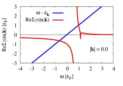
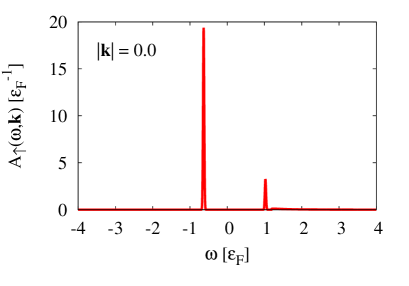
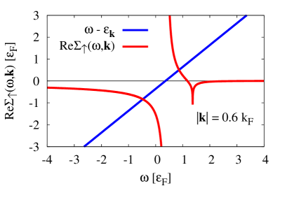
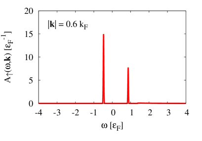
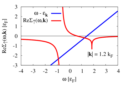
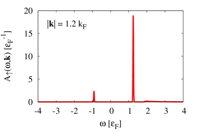
Figure 10: Left column: Real parts of the self-energy $\Sigma_{\uparrow}(\omega,\bm{k})$ [see Eq.(C.4)]. The intersections with the red line (${\rm Re}\Sigma=\omega-\epsilon_{\bm{k}}$) represent the peak positions of single-particle spectral densities [see Eq.(97)]. Right column: Single-particle spectral densities ${\cal A}_{\uparrow}(\omega,\bm{k})$ [see Eq.(96)]. For better visibility, the delta functions $\delta(\omega-\omega_{n})$ are approximated by $\sqrt{t/\pi}e^{-t(\omega-\omega_{n})^{2}}$ with $t=2000$. Each row from top to bottom corresponds to $|\bm{k}|/k_{F}=0.0$, $0.6$ and $1.2$.

Here the pole(s) $\omega=\omega_{n}(y)$ ($n=1,2,\cdots$) are the solution(s) of

$$\omega-\epsilon_{\bm{k}}-\Sigma_{\uparrow}(\omega+i0^{+},\bm{k})=0,$$ (97)

and the residue(s) $F_{n}(y)$ are given by

$$F_{n}^{-1}=1-\left.\frac{\partial\Sigma_{\uparrow}(\omega+i0^{+},\bm{k})}{\partial\omega}\right|_{\omega=\omega_{n}}.$$ (98)

Figure 10 shows the plots of ${\rm Re}\Sigma_{\uparrow}(\omega+i0^{+},\bm{k})$ and ${\cal A}_{\uparrow}(\omega,\bm{k})$, respectively, for $\xi=0.372$ and $\zeta=3.40$.

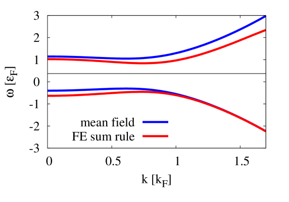
Figure 11: Peak positions of single-particle spectral densities in the $(|\bm{k}|,\omega)$ plane (red lines). For comparison, mean-field dispersion relations, $\omega=\xi\pm\sqrt{(\epsilon_{\bm{k}}-\xi)^{2}+C_{4}}$, are shown by the blue lines. The thin black line shows the position of $\omega=\xi$.

The peak positions of the single-particle spectral densities as functions of $|\bm{k}|$ are shown in Fig. 11, where, for comparison, we also show the mean-field dispersion relations, $\omega=\xi\pm\sqrt{(\epsilon_{\bm{k}}-\xi)^{2}+C_{4}}$. By investigating the point, at which the particle- and hole-branches approach each other most closely, we obtain a pairing gap value of $0.65\,\epsilon_{F}$, which is not much different from the mean-field result, $\sqrt{C_{4}}\simeq 0.68\,\epsilon_{F}$.

Appendix D The maximum entropy method

Let us here briefly recapitulate the basic steps of MEM and especially explain the differences of our analysis to the application of MEM to statistical Monte-Carlo data. For more details, consult for instance Gubler ; Gubler2 ; Jarrel ; Asakawa .

The problem to be solved with the help of MEM is given in Eqs.(27) and (28). As, however, the OPE on the right-hand side of these equations is only known with limited accuracy and is moreover only valid in a finite range of the Borel mass $M$, the problem of obtaining $\mathrm{Im}\Sigma_{\uparrow}(\omega,\bm{k})$ from the OPE is ill-posed and cannot be solved analytically.

MEM now uses Bayes’ theorem, by which additional information about $\mathrm{Im}\Sigma_{\uparrow}(\omega,\bm{k})$ such as positivity and its asymptotic behavior at large energies can be incorporated into the analysis and by which one then can extract the most probable from of $\mathrm{Im}\Sigma_{\uparrow}(\omega,\bm{k})$. Bayes’ theorem can be expressed as

$$P[\mathrm{Im}\Sigma|DH]=\frac{P[D|\mathrm{Im}\Sigma H]P[\mathrm{Im}\Sigma|H]}{P[D|H]},$$ (99)

where $H$ denotes prior knowledge of $\mathrm{Im}\Sigma_{\uparrow}(\omega,\bm{k})$ and $P[\mathrm{Im}\Sigma|DH]$ represents the conditional probability of $\mathrm{Im}\Sigma_{\uparrow}(\omega,\bm{k})$ for given $D^{\mathrm{OPE}}_{\uparrow}(M,\bm{k})$ and $H$. Maximizing the above functional with respect to $\mathrm{Im}\Sigma_{\uparrow}(\omega,\bm{k})$ will provide the most probable spectral function. $P[D|\mathrm{Im}\Sigma H]$ is called the “likelihood function” and is obtained as

$$\begin{split}P[D|\mathrm{Im}\Sigma H]&=e^{-L[\mathrm{Im}\Sigma]},\\ L[\mathrm{Im}\Sigma]&=\frac{1}{2(M_{\mathrm{max}}-M_{\mathrm{min}})}\displaystyle\int_{M_{\mathrm{min}}}^{M_{\mathrm{max}}}dM\frac{\bigl{[}D^{\mathrm{OPE}}_{n,\,\uparrow}(M,\bm{k})-D^{\mathrm{Im}\Sigma}_{n,\,\uparrow}(M,\bm{k})\bigr{]}^{2}}{\sigma_{n,\,\uparrow}^{2}(M,\bm{k})},\end{split}$$ (100)

with $n=0$ or $1$. Here, $D^{\mathrm{OPE}}_{n,\,\uparrow}(M,\bm{k})$ is given on the right-hand sides of Eqs.(27) or (28), while $D^{\mathrm{Im}\Sigma}_{n,\,\uparrow}(M,\bm{k})$ is defined as

$$D^{\mathrm{Im}\Sigma}_{n,\,\uparrow}(M,\bm{k})=\int_{-\infty}^{\infty}d\omega\mathcal{K}_{n}(\omega,M)\mathrm{Im}\Sigma_{\uparrow}(\omega,\bm{k}),$$ (101)

and hence implicitly depends on $\mathrm{Im}\Sigma_{\uparrow}(\omega,\bm{k})$. The error function $\sigma_{n,\,\uparrow}(M,\bm{k})$ stands for the uncertainty of $D^{\mathrm{OPE}}_{n,\,\uparrow}(M,\bm{k})$ at Borel mass $M$ and momentum $|{\bm{k}}|$, which we determine from the uncertainties of the parameters $\xi$ and $\zeta$ (e.g. the Bertsch parameter and the contact density) appearing in the OPE.

$P[\mathrm{Im}\Sigma|H]$ on the other hand is called the “prior probability” and can be written down as follows:

$$\begin{split}P[\mathrm{Im}\Sigma|H]&=e^{\alpha S[\mathrm{Im}\Sigma]},\\ S[\mathrm{Im}\Sigma]&=\displaystyle\int_{-\infty}^{\infty}d\omega\Bigr{[}\mathrm{Im}\Sigma_{\uparrow}(\omega,\bm{k})-m(\omega)-\mathrm{Im}\Sigma_{\uparrow}(\omega,\bm{k})\log\Bigl{(}\frac{\mathrm{Im}\Sigma_{\uparrow}(\omega,\bm{k})}{m(\omega)}\Bigr{)}\Bigl{]}.\end{split}$$ (102)

$S[\mathrm{Im}\Sigma]$ is known as the Shannon-Jaynes entropy and the function $m(\omega)$ is the so-called “default model”. In case of no available data $D^{\mathrm{OPE}}_{n,\,\uparrow}(M,\bm{k})$ or infinitely large error $\sigma_{n,\,\uparrow}(M,{\bm{k}})$, the MEM procedure will just give $m(\omega)$ for $\mathrm{Im}\Sigma_{\uparrow}(\omega,\bm{k})$ because this function maximizes $P[\mathrm{Im}\Sigma|H]$. The default model can thus be utilized to incorporate already known information about $\mathrm{Im}\Sigma_{\uparrow}(\omega,{\bm{k}})$ into the analysis.

Collecting all the terms discussed above, we reach the final form of the probability $P[\mathrm{Im}\Sigma|DH]$:

$$\begin{split}P[\mathrm{Im}\Sigma|DH]&\propto P[D|\mathrm{Im}\Sigma H]P[\mathrm{Im}\Sigma|H]\\ &=e^{Q[\mathrm{Im}\Sigma]},\\ Q[\mathrm{Im}\Sigma]&\equiv\alpha S[\mathrm{Im}\Sigma]-L[\mathrm{Im}\Sigma].\end{split}$$ (103)

It is now merely a numerical problem to obtain the form of $\mathrm{Im}\Sigma_{\uparrow}(\omega,{\bm{k}})$ that maximizes $Q[\mathrm{Im}\Sigma]$ and is therefore the most probable $\mathrm{Im}\Sigma_{\uparrow}(\omega,{\bm{k}})$ for given $D^{\mathrm{OPE}}_{n,\,\uparrow}(M,\bm{k})$ and $H$. For this task, we will use the Bryan algorithm Bryan .

Once $\mathrm{Im}\Sigma_{\alpha,\,\uparrow}(\omega,{\bm{k}})$ maximizing $Q[\mathrm{Im}\Sigma]$ for a fixed value of $\alpha$ is found, it is integrated out by averaging $\mathrm{Im}\Sigma_{\alpha,\,\uparrow}(\omega,{\bm{k}})$ over a certain range of $\alpha$, which then leads to our final result. Explicit formulae for this step and all other practical details specific to the application of MEM to QCD sum rules are discussed in Gubler ; Gubler2 .

As a final point, let us mention here that Eqs.(27) and (28) give two independent sum rules, which have to be combined in the analysis of this work. How this can be done is explained in Gubler2 .

References

- (1) I. Bloch, J. Dalibard, and W. Zwerger, Rev. Mod. Phys. 80, 885 (2008).
- (2) S. Giorgini, L.P. Pitaevskii, and S. Stringari, Rev. Mod. Phys. 80, 1215 (2008).
- (3) W. Zwerger (Editor), The BCS-BEC Crossover and the Unitary Fermi Gas, Lecture Notes in Physics, Springer (2011).
- (4) J.T. Stewart, J.P. Gaebler and D.S. Jin, Nature (London) 454, 744 (2008).
- (5) T.L. Dao, A. Georges, J. Dalibard, C. Salomon and I. Carusotto, Phys. Rev. Lett. 98, 240402 (2007).
- (6) R. Haussmann, M. Punk and W. Zwerger, Phys. Rev. A 80, 063612 (2009).
- (7) P. Magierski, G. Wlazlowski and A. Bulgac, Phys. Rev. Lett. 107, 145304 (2011).
- (8) J. Carlson and S. Reddy, Phys. Rev. Lett. 95, 060401 (2005).
- (9) K.G. Wilson, Phys. Rev. 179, 1499 (1969).
- (10) L.P. Kadanoff, Phys. Rev. Lett. 23, 1430 (1969).
- (11) A.M. Polyakov, Zh. Eksp. Teor. Fiz. 57, 271 (1969).
- (12) T. Muta, Foundations of quantum chromodynamics (World Scientific, Singapore, 1998).
- (13) M.A. Shifman MA, A.I. Vainshtein and V.I. Zakharov, Nucl. Phys. B147, 385 (1979).
- (14) M.A. Shifman MA, A.I. Vainshtein and V.I. Zakharov, Nucl. Phys. B147, 448 (1979).
- (15) E. Braaten and L. Platter, Phys. Rev. Lett. 100, 205301 (2008).
- (16) E. Braaten, D. Kang and L. Platter, Phys. Rev. A 78, 053606 (2008).
- (17) E. Braaten, D. Kang and L. Platter, Phys. Rev. Lett. 104, 223004 (2010).
- (18) E. Braaten, D. Kang and L. Platter, Phys. Rev. Lett. 106, 153005 (2011).
- (19) E. Braaten, in The BCS-BEC Crossover and the Unitary Fermi Gas, Lecture Notes in Physics, edited by W. Zwerger, Chap. 6 (Springer, Berlin, 2012).
- (20) D.T. Son and E.G. Thompson, Phys. Rev. A 81, 063634 (2010).
- (21) M. Barth and W. Zwerger, Ann. Phys. (NY) 326, 2544 (2011).
- (22) J. Hofmann, Phys. Rev. A 84, 043603 (2011).
- (23) W.D. Goldberger and I.Z. Rothstein, Phys. Rev. A 85, 013613 (2012).
- (24) W.D. Goldberger and Z.U. Khandker, Phys. Rev. A 85, 013624 (2012).
- (25) Y. Nishida, Phys. Rev. A 85, 053643 (2012).
- (26) S. Golkar and D.T. Son, JHEP 1412, 063 (2014).
- (27) W.D. Goldberger, Z.U. Khandker and S. Prabhu, arXiv:1412.8507 [hep-th].
- (28) S. Tan, Ann. Phys. 323, 2952 (2008).
- (29) S. Tan, Ann. Phys. 323, 2971 (2008).
- (30) S. Tan, Ann. Phys. 323, 2987 (2008).
- (31) M.J.H. Ku, A.T. Sommer, L.W. Cheuk and M.W. Zwierlein, Science 335, 563 (2012).
- (32) G. Zrn et al., Phys. Rev. Lett. 110, 135301 (2013).
- (33) S. Hoinka et al., Phys. Rev. Lett. 110, 055305 (2013).
- (34) J. Carlson, S. Gandolfi, K.E. Schmidt and S. Zhang, Phys. Rev. A 84, 061602(R) (2011).
- (35) S. Gandolfi, K.E. Schmidt and J. Carlson, Phys. Rev. A 83, 041601(R) (2011).
- (36) P. Gubler and M. Oka, Prog. Theor. Phys. 124, 995 (2010).
- (37) N.V. Krasnikov, A.A. Pivovarov and N.N. Tavkhelidze, Z. Phys. C 19, 301 (1983).
- (38) R.A. Bertlmann, G. Launer and E. de Rafael, Nucl. Phys. B250, 61 (1985).
- (39) G. Orlandini, T.G. Steele and D. Harnett, Nucl. Phys. A686, 261 (2001).
- (40) K. Ohtani, P. Gubler and M. Oka, Eur. Phys. J. A 47, 114 (2011).
- (41) B.L. Ioffe and K.N. Zyablyuk, Nucl. Phys. A687, 437 (2001).
- (42) K.J. Araki, K. Ohtani, P. Gubler and M. Oka, Prog. Theor. Exp. Phys. 2014 073B03 (2014).
- (43) P. Gubler, K. Morita and M. Oka, Phys. Rev. Lett. 107, 092003 (2011).
- (44) P. Gubler, A Bayesian Analysis of QCD Sum Rules, Springer Theses, Springer Japan, 2013.
- (45) K. Suzuki, P. Gubler, K. Morita and M. Oka, Nucl. Phys. A897, 28 (2013).
- (46) K. Ohtani, P. Gubler and M. Oka, Phys. Rev. D 87, 034027 (2013).
- (47) P. Gubler and K. Ohtani, Phys. Rev. D 90 094002 (2014).
- (48) J.E. Drut, T.A. Lhde and T. Ten, Phys. Rev. Lett. 106, 205302 (2011).
- (49) M. Jarrell and J.E. Gubernatis, Phys. Rep. 269, 133 (1996).
- (50) M. Asakawa, T. Hatsuda, and Y. Nakahara, Prog. Part. Nucl. Phys. 46, 459 (2001).
- (51) R.K. Bryan, Eur. Biophys. J. 18, 165 (1990).