Gain-scheduled Leader-follower Tracking Control for Interconnected Parameter Varying Systems

Abstract

This paper considers the gain-scheduled leader-follower tracking control problem for a parameter varying complex interconnected system with directed communication topology and uncertain norm-bounded coupling between the agents. A gain-scheduled consensus-type control protocol is proposed and a sufficient condition is obtained which guarantees a suboptimal bound on the system tracking performance under this protocol. An interpolation technique is used to obtain a protocol schedule which is continuous in the scheduling parameter. The effectiveness of the proposed method is demonstrated using a simulation example.

Key words: Gain scheduling; leader-follower tracking control; interconnected parameter varying systems; interpolation technique

1 Introduction

In recent years, the topic of cooperative control has attracted much attention. The objective of the cooperative control problem is to propose distributed control laws to achieve a desired system behavior [1]. A related problem is that of synchronization of complex dynamical systems where all the components are controlled to exhibit a similar behavior by interconnecting them into a network [2, 3].

There are several approaches to the synchronization problem for complex systems consisting of many dynamic subsystems-agents. In the average consensus problem, which has received considerable attention in the last decade [4, 5], the objective is to synchronize all the agents to a common state. Another approach is to employ a suitable internal model for the system. For instance, it is shown in [6] that the existence of such an implicit internal model is necessary and sufficient for synchronization of a system of heterogeneous linear agents considered in that paper. However, the internal model approach does not directly address the overall system performance, since each system is controlled to follow its own internal model dynamics. In general, it may be difficult to determine an internal model that guarantees a good synchronization performance. Yet another approach is to designate one of the agents to serve as a leader, and design interconnections within the system so that the rest of the system follows the leader [7]; also, see [8] for a recent example. This idea leads to the leader-follower tracking problem, which is the main focus of this paper.

A common feature of many papers that consider the leader-follower problem is that the dynamics of agents are usually assumed to be dynamically decoupled [22, 23, 24, 25, 26, 27]. In many complex systems, however, interactions between subsystems are inevitable and must be taken into account [11]. Examples of systems with dynamical interactions between subsystems include spacecraft control systems and power systems [9]. For example, it was noted in [10] that weak uncertain couplings between generators is one of the reasons for dynamic instability in power systems and, therefore, they should not be neglected. This motivates us to consider the leader-follower tracking problem for interconnected systems. While we do not consider a specific application, our approach makes a step towards using consensus feedback for synchronization of such systems, compared to other contributions in the area of networked control systems which do not address the presence of interconnections.

In this paper, we are concerned with the leader-follower tracking problem for interconnected systems that depend on a time varying parameter. Analysis and control of linear parameter varying systems has attracted much attention in the last two decades due to their applications in flight control [12], turbofan engines and wind turbine systems [13, 14]. For example, an application of the distributed control approach to control and synchronization of wind generation systems modeled as parameter varying systems has been presented in [14]. Even though a discrete time model was considered in [14], parameter varying system modeling was motivated by the fact that the wind energy source driving wind turbines exhibits time-varying nature. In order to integrate a wind generation system into a power grid in a grid-friendly manner, the total power output of the wind turbines must be regulated to conform to a constant output. Each turbine then serves as a node and is controlled with respect to its power output by turning the blade pitch angle, and the value of the blade pitch angle is propagated through the communication network using the leader-follower algorithm. Thanks to this and many other potential applications, the theory of cooperative control for parameter varying systems has been gaining attention in recent years [15, 16].

The main contribution of this paper concerns the leader-follower control of parameter varying interconnected systems. A related problem, from the synchronization viewpoint, has been studied in [18, 19]. In the first reference, the synchronization problem is solved for heterogeneous systems which depend on the parameters in an affine fashion, under the assumption that the network of LPV agents allows for an internal model for synchronization while the agents are decoupled from each other. That is, the agents interact over the control protocol only. In [19], while the linear dependency on the parameter is not required, the leader is assumed to be given and be completely decoupled from the agents. In contrast with these references, we assume the leader to be chosen from the group of parameter varying agents; it is interconnected to the rest of the network, and the linear dependency on the parameter is not required.

The fact that the leader is interconnected with the followers makes it difficult to apply regular centralized tracking techniques to the problem under consideration. Many tracking techniques assume that the reference trajectory is generated by an exosystem or is a priori known, and is independent of the followers. This is not the case in this paper. Alternatively, a centralized tracking controller can be obtained by solving a stabilization problem for a large-scale system comprised of subsystems describing dynamics of individual tracking errors. This can be done by applying one of the existing centralized gain-scheduling robust control techniques, e.g., using the technique from [21]. However, in general the centralized controller obtained this way will not have a desired information structure. Indeed, a controller obtained in such a way will not generally guarantee that the information from subsystems that are not observed by a node is not required for feedback. One way to enforce such an information constraint is to employ a block diagonal Lyapunov function. This is the solution approach undertaken in this paper and is its main difference from solutions which could be obtained in a centralized setup.

Different from many papers that study synchronization of decoupled systems (including the above mentioned references [18, 19], also see [2, 3]), in the case of coupled systems, it is essential to distinguish the network representing the existing interactions between the subsystems (including interactions with the leader) from the network which realizes communication and control. This leads us to consider a two-network structure in this paper. The rationale for this is twofold. Firstly, our aim is to construct synchronization protocols for all agents excluding the leader, as we wish to avoid perturbing the leader dynamics (other than through an unavoidable physical coupling). Hence, the communication graph of the network must be different from the interconnection graph. The second reason is that the interconnection graph describes dynamical couplings between subsystems and thus may be different from the communication and control graph.

Our main result is a sufficient condition for the design of a gain-scheduled leader-follower control protocol for parameter varying multi-agent systems with directed control network topology and linear uncertain couplings subject to norm-bounded constraints. The condition involves checking feasibility of parameterized linear matrix inequalities (LMIs) at several operating points of the system. These LMIs serve as the basis for the design of a continuous (in the scheduling parameter) control protocol for coupled parameter varying systems, by interpolating consensus control protocols computed for those operating points; cf. [29, 19, 21]. Interpolation allows us to mitigate detrimental effects of transients arising when the system traverses from one operating condition to another.

The remainder of the paper proceeds as follows. In Section 2, we formulate the leader follower control problem for parameter varying coupled multi-agent systems and give some preliminaries. The main results are given in Section 3. Section 4 gives an example which illustrates the theory presented in the paper. Finally, the conclusions are given in Section 5.

2 Problem Formulation and Preliminaries

2.1 Interconnection and communication graphs

As stated in the introduction, in this paper we draw a distinction between the communication topology of the system used for control and the topology of interactions between subsystems. The example of the two-graph structure is shown in Fig. 1, where the edges of the interconnection graph are indicated by the solid lines and the edges of the communication graph are shown by the dashed lines. Both coupling and communication topologies are described in terms of directed graphs defined on the common node set $\mathcal{V}=\{0,\ldots,N\}$. Without loss of generality, node 0 will be assigned to be the leader of the network, while the nodes from the set $\mathcal{V}_{0}=\{1,\ldots,N\}$ will represent the followers. The coupling graph and the communication graph will be denoted as $\mathcal{G}^{\varphi}$ and $\mathcal{G}^{c}$, respectively.

The edge sets of both graphs are subsets of the set $\mathcal{V}\times\mathcal{V}$ and consist of pairs of nodes. The pair $(j,i)$ in each edge set denotes the directed edge which originates at node $j$ and ends at node $i$. Edge $(j,i)$ in the edge set of the directed coupling graph $\mathcal{G}^{\varphi}$, denoted $\mathcal{E}^{\varphi}$, describes the fact that node $i$ is influenced by node $j$ through a directed interaction between nodes $j$ and $i$.

Also, $\mathcal{E}^{c}\subseteq\mathcal{V}\times\mathcal{V}$ denotes an edge set of the communication graph $\mathcal{G}^{c}$, consisting of ordered pairs of nodes. Each such edge indicates the information flow between the nodes, that is, $(j,i)\in\mathcal{E}^{c}$ if and only if node $i$ obtains information from node $j$, which it can use for control.

The adjacency matrix of the directed interconnection graph $\mathcal{G}^{\varphi}$ is denoted as $\mathcal{A}^{\varphi}$, its $(i,j)$-th entry is 1 if and only if $(j,i)\in\mathcal{E}^{\varphi}$. The adjacency matrix $\mathcal{A}^{c}$ of the directed communication graph $\mathcal{G}^{c}$ is defined in the same manner. Since according to a standard convention we assume that both the coupling graph and communication graph have no self-loops, the diagonal entries of $\mathcal{A}^{\varphi}$ and $\mathcal{A}^{c}$ are all equal to zero.

To distinguish between the leader and the rest of the network, we define subgraphs $\mathcal{G}^{\varphi}_{0}$, $\mathcal{G}^{c}_{0}$ of the graphs $\mathcal{G}^{\varphi}$, $\mathcal{G}^{c}$ defined on the node set $\mathcal{V}_{0}=\{1,\ldots,N\}$, with the edge sets $\mathcal{E}_{0}^{\varphi}=\{(j,i)\in\mathcal{E}^{\varphi}\colon i,j\in\mathcal{V}_{0}\}$ and $\mathcal{E}_{0}^{c}=\{(j,i)\in\mathcal{E}^{c}\colon i,j\in\mathcal{V}_{0}\}$, respectively. Selecting the subgraphs $\mathcal{G}^{\varphi}_{0}$ and $\mathcal{G}^{c}_{0}$ induces the partition of the matrices $\mathcal{A}^{\varphi}$, $\mathcal{A}^{c}$,

$$\mathcal{A}^{\varphi}=\left[\begin{array}[]{c|c}0&\bar{d}\\ \hline\cr d&\mathcal{A}^{\varphi}_{0}\end{array}\right],\quad\mathcal{A}^{c}=\left[\begin{array}[]{c|c}0&0\\ \hline\cr g&\mathcal{A}^{c}_{0}\end{array}\right],$$

where $d=[d_{1}~{}\ldots~{}d_{N}]^{\prime}$, $\bar{d}=[\bar{d}_{1}~{}\ldots~{}\bar{d}_{N}]$, $g=[g_{1}~{}\ldots~{}g_{N}]^{\prime}$ and $\mathcal{A}^{\varphi}_{0}$, $\mathcal{A}^{c}_{0}$ are the adjacency matrices of the subgraphs $\mathcal{G}^{\varphi}_{0}$ and $\mathcal{G}^{c}_{0}$, respectively. The zero row of the matrix $\mathcal{A}^{c}$ reflects our assumption that the leader node does not receive the state information from other nodes of the network. However, the corresponding row of $\mathcal{A}^{\varphi}$ may be nonzero since the leader node may be physically coupled with some of the followers.

In this paper we are concerned with the case where only some of the followers receive the state information directly from the leader. We refer to such nodes $i\in\mathcal{V}_{0}$ as pinned nodes; the corresponding entries of the adjacency matrix $\mathcal{A}^{c}$, $g_{i}=1$, and $g_{i}=0$ if node $i$ is not pinned. The matrix $G=\mathrm{diag}\{g_{i}\}\in\Re^{N\times N}$ is referred to as a pinning matrix.

The Laplacian matrix of the subgraph $\mathcal{G}^{c}_{0}$ is defined as $\mathcal{L}^{c}_{0}=\mathcal{P}-\mathcal{A}^{c}_{0}$, where $\mathcal{P}=\mathrm{diag}\{p_{1},\ldots,p_{N}\}\in R^{N\times N}$ is the in-degree matrix of $\mathcal{G}^{c}_{0}$, i.e., the diagonal matrix, whose diagonal elements are the in-degrees of the corresponding nodes of the graph $\mathcal{G}^{c}_{0}$, $p_{i}=\sum_{j=1}^{N}a_{ij}^{c}$ for $i=1,\ldots,N$, where $a_{ij}^{c}$ are the elements of the $i$th row of the matrix $\mathcal{A}^{c}_{0}$.

Finally, we give the definition and the notation for neighborhoods in the above graphs.

Definition 1

$\mathcal{G}^{c}_{0}=(\mathcal{V},\mathcal{E}^{c})$ is a communication graph, each node $i\in\mathcal{V}$ represents a subsystem in the interconnected system and edge $(j,i)\in\mathcal{E}^{c}$ means that node $i$ obtain information from node $j$.

Definition 2

$\mathcal{G}^{\phi}$ is an interconnection graph, each node $i\in\mathcal{V}$ represents a subsystem in the interconnected system and edge $(j,i)\in\mathcal{E}^{\phi}$ indicates that subsystem $i$ is influenced by subsystem $j$ through a directed interaction between subsystems $i$ and $j$.

Node $j$ is called a neighbor of node $i$ in the graph $\mathcal{G}^{\varphi}$ (or $\mathcal{G}^{\varphi}_{0}$, $\mathcal{G}^{c}$, $\mathcal{G}^{c}_{0}$, respectively) if $(j,i)\in\mathcal{E}^{\varphi}$ ($\mathcal{E}_{0}^{\varphi},\mathcal{E}^{c}$ or $\mathcal{E}_{0}^{c}$, respectively). The sets of neighbors of node $i$ in the graphs $\mathcal{G}^{\varphi}$ and $\mathcal{G}^{c}$ are denoted as $N^{\varphi}_{i}=\{j|(j,i)\in\mathcal{E}^{\varphi}\}$, and $N^{c}_{i}=\{j|(j,i)\in\mathcal{E}^{c}\}$, respectively. The sets of neighbors of node $i$ in the subgraphs $\mathcal{G}^{\varphi}_{0}$ and $\mathcal{G}^{c}_{0}$ are denoted as $S^{\varphi}_{i}=\{j|(j,i)\in\mathcal{E}_{0}^{\varphi}\}$ and $S^{c}_{i}=\{j|(j,i)\in\mathcal{E}_{0}^{c}\}$, respectively.

We conclude this subsection by specifying our standing requirements on the communication topology of the network which are assumed to hold throughout the paper.

Assumption 1

The communication subgraph $\mathcal{G}_{0}^{c}$ contains a spanning tree, whose root node $i_{r}$ is the pinned node, i.e., $g_{i_{r}}>0$.

Remark 1

Assumption 1 ensures that the information flows from the leader to its pinned followers, as well as between other followers [25, 28].

Figure 1: An example of the interconnection and communication graphs.

2.2 Notation

Throughout the paper, the following notation will be used.

$\Re^{n}$ and $\Re^{n\times m}$ are a real Euclidean $n$-dimensional vector space and a space of real $n\times m$ matrices.

$\Gamma$ denotes an interval $[\rho_{\min},\rho_{\max}]\subset\Re$. The symbols $\rho$, $\rho_{s}$, $\bar{\rho}_{s}$, $\underline{\rho}_{s}$, etc., will represent various points within the interval $\Gamma$, and $\Gamma_{\ell}$, $\Gamma_{0}$ will denote sets of points within $\Gamma$ which will be defined later in the paper. Also, $\rho(t)$ is a scalar function, defined on $[0,\infty)$ and taking values in the interval $\Gamma$. This function will describe a time-varying scheduling parameter of the multi-agent system under consideration.

Unless stated otherwise, the notations $A(\rho)$, $Y_{\rho}$, etc., will refer to matrices of appropriate dimension parameterized by $\rho\in\Gamma$.

For $q\in\Re^{n}$, $\mathrm{diag}\{q\}$ denotes the diagonal matrix with the entries of $q$ as its diagonal elements.

$\otimes$ denotes the Kronnecker product of two matrices.

$\lambda_{\max}(\cdot)$ and $\lambda_{\min}(\cdot)$ will denote the largest and the smallest eigenvalues of a real symmetric matrix.

$I_{N}$ is the $N\times N$ identity matrix, and $\mathbf{1}_{N}\in\Re^{N}$ is the vector whose all entries are equal to $1$. When the dimension is clear from the context, the subscript $N$ will be suppressed, and $I$ will represent the identity matrix of an appropriate dimension.

For two symmetric matrices $X$ and $Y$ of the same dimensions, $X\geq Y$, ($X>Y$) if and only if $X-Y$ is positive semidefinite (positive definite).

Consider the Laplacian matrix of the subgraph $\mathcal{G}^{c}_{0}$, $\mathcal{L}^{c}_{0}$. According to [28], under Assumption 1, the matrix $\mathcal{L}^{c}_{0}+G$ is nonsingular (also see [27]), and all the entries of the vector $\vartheta=[\vartheta_{1},\ldots,\vartheta_{N}]^{\prime}=(\mathcal{L}^{c}_{0}+G)^{-1}\textbf{1}_{N}$ are positive. Also, the matrix $\Theta^{-1}(\mathcal{L}^{c}_{0}+G)+(\mathcal{L}^{c}_{0}+G)^{\prime}\Theta^{-1}$ is positive definite, where $\Theta\triangleq\mathrm{diag}\{\vartheta\}$. The following two constants will be used in the proofs of our results:

$$\sigma = \frac{1}{2}\lambda_{\min}\left(\Theta^{-1}(\mathcal{L}^{c}_{0}+G)+(\mathcal{L}^{c}_{0}+G)^{\prime}\Theta^{-1}\right),$$

$$\hat{\lambda} = \lambda_{\max}\left((\mathcal{L}^{c}_{0}+G)^{\prime}\Theta^{-2}(\mathcal{L}^{c}_{0}+G)\right).$$ (2)

2.3 Problem Formulation

The system under consideration consists of $N+1$ parameter-varying dynamical agents, coupled with their neighbors; the topology of interconnections is captured by the directed graph $\mathcal{G}^{\varphi}$. Dynamics of the $i$th agent are described by the linear equation

$$\dot{x}_{i}=A(\rho(t))x_{i}+B_{1}u_{i}+B_{2}\sum\limits_{j\in N^{\varphi}_{i}}\varphi_{ij}(t,x_{j}-x_{i}),\quad i=0,\ldots,N,$$ (3)

where $x_{i}\in\Re^{n}$ is the state of agent $i$, $u_{i}\in\Re^{p}$ is the control input and $\rho(t)$ is the time-varying parameter, which is available to all agents. It is assumed that $\rho\colon[0,\infty)\rightarrow\Gamma\subset\Re$ is a continuous function. Also in equation (3), $B_{1}$ and $B_{2}$ are real matrices of appropriate dimensions, and $A(\rho(t))$ is the composition of a continuous matrix-valued function $A(\cdot)\colon\Gamma\to\Re^{n\times n}$ and the function $\rho(t)$ defined above.

The functions $\varphi_{ij}\colon[0,\infty)\times\Re^{n}\to\Re^{m}$,

$$\varphi_{ij}(t,x)=\Delta_{ij}(t)C_{ij}x,\quad x\in\Re^{n},$$

describe how agent $j$ influences the dynamics of agent $i$. Here $C_{ij}\in\Re^{q_{ij}\times n}$ and $\Delta_{ij}\in\Re^{m\times q_{ij}}$ are respectively constant and time-varying matrices. According to the above model, we focus on linear time-varying interactions between the subsystems whose strengths depend on the relative state of subsystem $i$ with respect to subsystem $j$, $x_{j}-x_{i}$. Also, we will assume that the coefficients $\Delta_{ij}(t)$ are uncertain, and satisfy the constraint

$$\Delta_{ij}^{\prime}(t)\Delta_{ij}(t)\leq I,\quad\forall t\in[0,\infty).$$ (4)

That is, we consider a class of norm-bounded uncertain interactions, which will be denoted by $\Xi$.

Since we have designated agent 0 to be the leader, and the rest of the agents to be controlled are to follow the leader, then according to (3) dynamics of the $i$th follower are described by the equation

$$\dot{x}_{i}= A(\rho(t))x_{i}+B_{1}u_{i}+B_{2}\Big{(}\sum\limits_{j\in S^{\varphi}_{i}}\varphi_{ij}(t,x_{j}-x_{i})+d_{i}\varphi_{i0}(t,x_{0}-x_{i})\Big{)},\quad i=1,\ldots,N,$$ (5)

while the leader dynamics are given by the equation

$$\dot{x}_{0}=A(\rho(t))x_{0}+B_{2}\sum\limits_{k\colon\bar{d}_{k}=1}\varphi_{0k}(t,x_{k}-x_{0}).$$ (6)

Unlike agents $i$, $i=1,\ldots N$, the leader is not controlled, i.e., $u_{0}\equiv 0$. On the contrary, all other agents will be controlled to track node 0.

Remark 2

In this paper, no a priori stability assumptions are made about the matrices $A(\rho)$. This is in contrast to, for example, the synchronization problem considered in [22], where the dynamics of the leader were required to be stable or marginally stable. In the sequel, however, certain conditions, in an LMI form, will be imposed on the coefficients of the leader and followers dynamics. While we formally make no special provisions regarding these coefficients, except for the feasibility of these LMI conditions, for such LMIs to be feasible one can reasonably expect the overall system dynamics to have certain collective stabilizability and detectability properties; see Remark 3 below.

Define tracking performance associated with the control input $u(\cdot)=[u_{1}(\cdot)^{\prime}~{}\ldots~{}u_{N}(\cdot)^{\prime}]^{\prime}$ as

$$\mathcal{J}(u) =\sum\limits_{i=1}^{N}\int_{0}^{\infty}\left((x_{0}-x_{i})^{\prime}Q(x_{0}-x_{i})+u_{i}^{\prime}Ru_{i}\right)dt,$$ (7)

where $Q=Q^{\prime}>0$ and $R=R^{\prime}>0$ are given weighting matrices. In this paper we are concerned with the following problem.

Problem 1

For each follower $i$, find gain schedule functions $K_{i}\colon\Gamma\to\Re^{p\times n}$ so that the control protocols of the form

$$u_{i}=-K_{i}(\rho(t))\left\{\sum\limits_{j\in S^{c}_{i}}(x_{j}-x_{i})+g_{i}(x_{0}-x_{i})\right\},$$ (8)

ensure a bounded worst-case tracking performance,

$$\sup\limits_{\Xi}\mathcal{J}(u)<\mathrm{const},$$ (9)

where $\mathrm{const}$ denotes a constant which can depend on $x_{0}(0)$ and $x_{i}(0)$.

3 The Main Results

In this section, we first revisit the leader follower tracking control problem for multi-agent systems with fixed parameters considered in [17] to obtain a sufficient condition for the design of a control protocol for a more general class of systems involving coupling between the leader and the agents. This sufficient condition will then be applied to develop an interpolation technique to obtain a continuous gain scheduling tracking control protocol for the system (3). The interpolation technique is the main result of this paper.

3.1 Leader follower control for fixed parameter systems

We now revisit the results of [17]. This revision is prompted by a more general structure of the system (3) which allows for physical connections between the leader and the followers. As a result, the form of the control protocol is somewhat different here in that the resulting controller gains depend on $i$.

Consider a fixed-parameter version of the system (3) described by the equation

$$\dot{x}_{i}= A(\rho)x_{i}+\beta\xi_{i}(t,x_{i})+B_{1}u_{i}+B_{2}\sum\limits_{j\in N^{\varphi}_{i}}\varphi_{ij}(t,x_{j}-x_{i}),\quad i=0,\ldots,N,$$ (10)

where $\rho\in\Gamma$ is fixed, and $\beta$ is a positive constant. Compared to (3), the system (10) includes an additional uncertainty element $\xi_{i}(t,x_{i})$, which satisfies the following constraint

$$\|\xi_{0}(t,x)-\xi_{i}(t,y)\|^{2}\leq\|x-y\|^{2},\quad\forall x,y\in\Re^{n}.$$ (11)

In the sequel, we will show that when the difference $A(\rho(t))-A(\rho)$ is sufficiently small, the system (3) can be represented as the system (10) subject to (11).

We now derive a distributed protocol of the form (8) under which the fixed-parameter uncertain system (10) satisfies the performance requirement (9).

Define the leader tracking error vectors as $e_{i}=x_{0}-x_{i}$, $i=1,\ldots,N$. Dynamics of the variable $e_{i}$ satisfy the equation

$$\dot{e}_{i}= A(\rho)e_{i}-B_{1}u_{i}+\beta\tilde{\xi}_{i}(t)-B_{2}\sum\limits_{k\colon\bar{d}_{k}=1}\varphi_{0k}(t,e_{k})$$

$$-B_{2}\sum\limits_{j\in S^{\varphi}_{i}}\big{(}\varphi_{ij}(t,e_{i})-\varphi_{ij}(t,e_{j})\big{)}-B_{2}d_{i}\varphi_{i0}(t,e_{i}),$$ (12)

where $\tilde{\xi}_{i}(t)\triangleq\xi_{0}(t,x_{0}(t))-\xi_{i}(t,x_{i}(t))$. It follows from (11) that $\|\tilde{\xi}_{i}\|^{2}\leq\|e_{i}\|^{2}$ for all $t\geq 0$.

For node $i$ of the subgraph $\mathcal{G}^{\varphi}_{0}$, introduce matrices $\hat{C}_{i}=[C_{ij_{1}}^{\prime}\ldots C_{ij_{\kappa_{i}}}^{\prime}]^{\prime}$, $\bar{C}_{i}=[C_{r_{1}i}^{\prime}\ldots C_{r_{\chi_{i}}i}^{\prime}]^{\prime}$, where $j_{1},\ldots,j_{\kappa_{i}}$ are the elements of the neighborhood set $S^{\varphi}_{i}$, and $r_{1},\ldots,r_{\chi_{i}}$ are the nodes with the property $(i,r_{\iota})\in\mathcal{E}^{\varphi}_{0}$; $\kappa_{i}$ and $\chi_{i}$ are, respectively, the in-degree and the out-degree of node $i$ in the graph $\mathcal{G}^{\varphi}_{0}$. Also, let $\bar{Q}=(\sigma^{2}/\hat{\lambda})Q$, where $\sigma$, $\hat{\lambda}$ are the constants defined in (2).

In order to formulate the extension of Theorem 1 in [17], with each node $i$, $i=1,\dots,N$, we associate a collection of positive constants $\nu_{ij}$, $\mu_{ij}$, $j\in S^{\varphi}_{i}$, $\pi_{i}$, $\nu_{i0}$ (only for those nodes $i$ for which $d_{i}=1$), and $\mu_{0i}$ (only for those nodes $i$ for which $\bar{d}_{i}=1$). Also, let $Y=Y^{\prime}>0$ be an $n\times n$ matrix. Using these constants and the matrix, for each node $i$ introduce a matrix $\Pi_{i}$ defined depending on $d_{i}$, $\bar{d}_{i}$ as follows.

Case 1. $d_{i}\neq 0$ and $\bar{d}_{i}\neq 0$. For each such node $i$, define the matrix $\Pi_{i}$ as

$$\scriptsize\Pi_{i}=\left[\begin{array}[]{ccccc|cc}Z_{i}&Y\bar{Q}^{1/2}&Y\hat{C}_{i}^{\prime}&Y\bar{C}_{i}^{\prime}&Y&YC_{i0}^{\prime}&YC_{0i}^{\prime}\\ \bar{Q}^{1/2}Y&-I&0&0&0&0&0\\ \hat{C}_{i}Y&0&-\Phi_{i}&0&0&0&0\\ \bar{C}_{i}Y&0&0&-\Omega_{i}&0&0&0\\ Y&0&0&0&-\Lambda_{i}&0&0\\[2.0pt] \hline\cr C_{i0}Y&0&0&0&0&-\frac{1}{\nu_{i0}}I&0\\ C_{0i}Y&0&0&0&0&0&-\frac{1}{N\mu_{0i}}I\end{array}\right],$$ (20)

where

$$\Phi_{i}= \mathrm{diag}[\frac{1}{\nu_{ij}}I,j\in S^{\varphi}_{i}],\quad\Omega_{i}=\mathrm{diag}[\frac{1}{\mu_{ji}}I,j\colon i\in S^{\varphi}_{j}],\quad\Lambda_{i}=\frac{1}{\pi_{i}}I,$$

$$Z_{i}= A(\rho)Y+YA(\rho)^{\prime}-B_{1}R^{-1}B_{1}^{\prime}+\frac{1}{\pi_{i}}\beta^{2}I$$

$$+\big{(}\sum\limits_{j\in S^{\varphi}_{i}}(\frac{1}{\nu_{ij}}+\frac{1}{\mu_{ij}})+\frac{1}{\nu_{i0}}+\sum\limits_{k\colon\bar{d}_{k}=1}\frac{1}{\mu_{0k}}\big{)}B_{2}B_{2}^{\prime}.\quad$$ (21)

Case 2. $d_{i}=0$ and $\bar{d}_{i}\neq 0$. For each such node $i$, the constant $\nu_{i0}$ is not defined. Accordingly, we define the matrix $\Pi_{i}$ by removing the second last column and row from the matrix in (20):

$$\Pi_{i}=\left[\begin{array}[]{ccccc|c}Z_{i}&Y\bar{Q}^{1/2}&Y\hat{C}_{i}^{\prime}&Y\bar{C}_{i}^{\prime}&Y&YC_{0i}^{\prime}\\ \bar{Q}^{1/2}Y&-I&0&0&0&0\\ \hat{C}_{i}Y&0&\Phi_{i}&0&0&0\\ \bar{C}_{i}Y&0&0&\Omega_{i}&0&0\\ Y&0&0&0&\Lambda_{i}&0\\ \hline\cr C_{0i}Y&0&0&0&0&-\frac{1}{N\mu_{0i}}I\end{array}\right],$$ (28)

where the matrix $Z_{i}$ is modified to be

$$Z_{i}=A(\rho)Y+YA(\rho)^{\prime}-B_{1}R^{-1}B_{1}^{\prime}+\frac{1}{\pi_{i}}\beta^{2}I+\big{(}\sum\limits_{j\in S^{\varphi}_{i}}(\frac{1}{\nu_{ij}}+\frac{1}{\mu_{ij}})+\sum\limits_{k\colon\bar{d}_{k}=1}\frac{1}{\mu_{0k}}\big{)}B_{2}B_{2}^{\prime}.$$ (29)

Case 3. $d_{i}\neq 0$ and $\bar{d}_{i}=0$. For each such node the constant $\mu_{0i}$ is not defined, hence the corresponding matrix $\Pi_{i}$ will be defined by removing the last column and row from the matrix in (20):

$$\Pi_{i}=\left[\begin{array}[]{ccccc|c}Z_{i}&Y\bar{Q}^{1/2}&Y\hat{C}_{i}^{\prime}&Y\bar{C}_{i}^{\prime}&Y&YC_{i0}^{\prime}\\ \bar{Q}^{1/2}Y&-I&0&0&0&0\\ \hat{C}_{i}Y&0&-\Phi_{i}&0&0&0\\ \bar{C}_{i}Y&0&0&-\Omega_{i}&0&0\\ Y&0&0&0&-\Lambda_{i}&0\\[2.0pt] \hline\cr C_{i0}Y&0&0&0&0&-\frac{1}{\nu_{i0}}I\end{array}\right],$$ (36)

The matrix $Z_{i}$ is the same as in (21).

Case 4. $d_{i}=0$ and $\bar{d}_{i}=0$. In this case, both $\nu_{i0}$ and $\mu_{0i}$ are not defined, and the corresponding matrix $\Pi_{i}$ is defined by removing two last columns and rows from the matrix in (20):

$$\Pi_{i}=\left[\begin{array}[]{ccccc}Z_{i}&Y\bar{Q}^{1/2}&Y\hat{C}_{i}^{\prime}&Y\bar{C}_{i}^{\prime}&Y\\ \bar{Q}^{1/2}Y&-I&0&0&0\\ \hat{C}_{i}Y&0&-\Phi_{i}&0&0\\ \bar{C}_{i}Y&0&0&-\Omega_{i}&0\\ Y&0&0&0&-\Lambda_{i}\end{array}\right],$$ (42)

The matrix $Z_{i}$ is the same as in (29).

The following theorem is an extension of Theorem 1 in [17].

Theorem 1

Under Assumption 1, let a matrix $Y=Y^{\prime}>0$, $Y\in\Re^{n\times n}$, constants $\nu_{ij}>0$, $\mu_{ij}>0$, $\pi_{i}>0$, $j\in S^{\varphi}_{i}$, $i=1,\ldots,N$, and constants $\nu_{i0}>0$ (for those $i$ with $d_{i}\neq 0$), $\mu_{0i}>0$ (for those $i$ with $\bar{d}_{i}\neq 0$) exist such that the following LMIs are satisfied simultaneously

$$\Pi_{i}<0,\quad i=1,\ldots,N.$$ (43)

Then the control protocol (8) with

$$K_{i}(\rho)=-(\vartheta_{i}\sigma)^{-1}R^{-1}B_{1}^{\prime}Y^{-1}$$ (44)

solves the leader follower tracking control problem for the fixed parameter system (10). Furthermore, this protocol guarantees the following performance bound

$$\sup_{\Xi}\mathcal{J}(u)\leq\frac{\hat{\lambda}}{\sigma^{2}}\sum_{i=1}^{N}(x_{0}(0)-x_{i}(0))^{\prime}Y^{-1}(x_{0}(0)-x_{i}(0))$$ (45)

for all uncertainties $\xi_{i}$ for which (11) holds.

Remark 3

The feasibility of the LMIs (43) in Theorem 1 is a sufficient condition for the existence of a control scheme to guarantee the performance bound (45). The LMIs are numerically tractable and can be solved using the existing software. Additionally, using the standard tools of the $H_{\infty}$ control theory, such as the Strict Bounded Real Lemma and the associated Riccati equation, the feasibility of the LMIs (43) can be related to collective stabilizability and/or detectability properties of the coefficients of the interconnected system (10). Since this system consists of identical agents, one can expect that each agent must necessarily have corresponding stabilizability and detectability properties for these collective properties to hold; cf. [20].

Proof: Using the Schur complement, each LMI (43) can be transformed into the following Riccati inequality:

$$A(\rho)Y+YA(\rho)^{\prime}-B_{1}R^{-1}B_{1}^{\prime}+\big{(}\sum\limits_{j\in S^{\varphi}_{i}}(\frac{1}{\nu_{ij}}+\frac{1}{\mu_{ij}})+\sum\limits_{k\colon\bar{d}_{k}=1}\frac{1}{\mu_{0k}}\big{)}B_{2}B_{2}^{\prime}+\frac{1}{\pi_{i}}\beta^{2}I$$

$$+Y\big{(}\bar{Q}+\sum\limits_{j\in S^{\varphi}_{i}}\nu_{ij}C^{\prime}_{ij}C_{ij}+\sum\limits_{j\colon i\in S^{\varphi}_{j}}\mu_{ji}C^{\prime}_{ji}C_{ji}+\pi_{i}I\big{)}Y$$

$$+\left(\frac{1}{\nu_{i0}}B_{2}B_{2}^{\prime}+\nu_{i0}YC^{\prime}_{i0}C_{i0}Y\right)$$

(this term is present only if $$d_{i}=1$$)

$$+N\mu_{0i}YC^{\prime}_{0i}C_{0i}Y<0$$ (46)

$$\qquad\qquad\qquad\mbox{(this term is present only if $\bar{d}_{i}=1$)}.$$

Note that the last and the second last lines in the Riccati inequality (3.1) are present only for those nodes $i$ for which $d_{i}\neq 0$ and/or $\bar{d}_{i}\neq 0$, respectively.

After pre- and post-multiplying (3.1) by $Y^{-1}$, and then using the expression (44) for $K_{i}(\rho)$ in the resulting inequality, we obtain

$$Y^{-1}(A(\rho)+\sigma\vartheta_{i}B_{1}K_{i}(\rho))+(A(\rho)+\sigma\vartheta_{i}B_{1}K_{i}(\rho))^{\prime}Y^{-1}+\sum\limits_{j\in S^{\varphi}_{i}}\nu_{ij}C^{\prime}_{ij}C_{ij}+\sum\limits_{j\colon i\in S^{\varphi}_{j}}\mu_{ji}C^{\prime}_{ji}C_{ji}$$

$$+Y^{-1}\Big{(}\big{(}\sum\limits_{j\in S^{\varphi}_{i}}(\frac{1}{\nu_{ij}}+\frac{1}{\mu_{ij}})+\sum\limits_{k\colon\bar{d}_{k}=1}\frac{1}{\mu_{0k}}\big{)}B_{2}B_{2}^{\prime}+\frac{1}{\pi_{i}}\beta^{2}I\Big{)}Y^{-1}+Y^{-1}B_{1}R^{-1}B_{1}^{\prime}Y^{-1}+\bar{Q}+\pi_{i}I$$

$$+\left(\frac{1}{\nu_{i0}}Y^{-1}B_{2}B_{2}^{\prime}Y^{-1}+\nu_{i0}C^{\prime}_{i0}C_{i0}\right)$$

(this term is present only if $$d_{i}=1$$)

$$+N\mu_{0i}C^{\prime}_{0i}C_{0i}<0$$ (47)

$$\qquad\qquad\qquad\mbox{(this term is present only if $\bar{d}_{i}=1$)}.$$

Define $e=[e^{\prime}_{1},\ldots,e^{\prime}_{N}]^{\prime}$ and consider the following Lyapunov function candidate for the interconnected system consisting of the subsystems (3.1):

$$V(e)=\sum\limits_{i=1}^{N}e_{i}^{\prime}Y^{-1}e_{i}.$$ (48)

Then

$$\frac{dV(e)}{dt}= \sum\limits_{i=1}^{N}2e_{i}^{\prime}Y^{-1}\Big{(}A(\rho)e_{i}+B_{1}K_{i}(\rho)(\sum\limits_{j\in S^{c}_{i}}(e_{i}-e_{j})+g_{i}e_{i})\Big{)}$$

$$-2\sum\limits_{i=1}^{N}\sum\limits_{k\colon\bar{d}_{k}=1}e_{i}^{\prime}Y^{-1}B_{2}\varphi_{0k}(t,e_{k})+2\sum\limits_{i=1}^{N}e_{i}^{\prime}Y^{-1}\beta\tilde{\xi}_{i}(t,e_{i})-2\sum\limits_{i=1}^{N}d_{i}e_{i}^{\prime}Y^{-1}B_{2}\varphi_{i0}(t,e_{i})$$

$$-2\sum\limits_{i=1}^{N}\sum\limits_{j\in S^{\varphi}_{i}}e_{i}^{\prime}Y^{-1}B_{2}\varphi_{ij}(t,e_{i})+2\sum\limits_{i=1}^{N}\sum\limits_{j\in S^{\varphi}_{i}}e_{i}^{\prime}Y^{-1}B_{2}\varphi_{ij}(t,e_{j}).$$ (49)

Note the following inequality:

$$\sum\limits_{i=1}^{N}2e_{i}^{\prime}Y^{-1}B_{1}K_{i}(\rho)(\sum\limits_{j\in S^{c}_{i}}(e_{i}-e_{j})+g_{i}e_{i})$$

$$=-2e^{\prime}(\Theta(\mathcal{L}^{c}_{0}+G)\otimes(Y^{-1}B_{1}(\sigma R)^{-1}B_{1}^{\prime}Y^{-1}))e$$

$$=-y^{\prime}\big{(}(\Theta(\mathcal{L}^{c}_{0}+G)+(\mathcal{L}^{c}_{0}+G)^{\prime}\Theta)\otimes I_{p}\big{)}y$$

$$\leq-2\sigma y^{\prime}\big{(}I_{N}\otimes I_{p}\big{)}y$$

$$=-2\sigma e^{\prime}\big{(}I_{N}\otimes Y^{-1}B_{1}(\sigma R)^{-1}B_{1}^{\prime}Y^{-1}\big{)}e$$

$$=-2\sum\limits_{i=1}^{N}e_{i}^{\prime}Y^{-1}B_{1}R^{-1}B_{1}^{\prime}Y^{-1}e_{i},$$ (50)

where $y=(I_{N}\otimes(\sigma R)^{-1/2}B_{1}^{\prime}Y^{-1})e$.

From (3.1) and (3.1), one has

$$\frac{dV(e)}{dt}\leq \sum\limits_{i=1}^{N}2e_{i}^{\prime}Y^{-1}\Big{(}A(\rho)+\sigma\vartheta_{i}B_{1}K_{i}(\rho)\Big{)}e_{i}+2\sum\limits_{i=1}^{N}e_{i}^{\prime}Y^{-1}\beta\tilde{\xi}_{i}(t,e_{i})$$

$$-2\sum\limits_{i=1}^{N}\sum\limits_{j\in S^{\varphi}_{i}}e_{i}^{\prime}Y^{-1}B_{2}\varphi_{ij}(t,e_{i})-2\sum\limits_{i=1}^{N}\sum\limits_{k\colon\bar{d}_{k}=1}e_{i}^{\prime}Y^{-1}B_{2}\varphi_{0k}(t,e_{k})$$

$$-2\sum\limits_{i=1}^{N}d_{i}e_{i}^{\prime}Y^{-1}B_{2}\varphi_{i0}(t,e_{i})+2\sum\limits_{i=1}^{N}\sum\limits_{j\in S^{\varphi}_{i}}e_{i}^{\prime}Y^{-1}B_{2}\varphi_{ij}(t,e_{j}).$$ (51)

Using the Riccati inequality (3.1), it follows from (3.1) that

$$\frac{dV(e)}{dt}\leq -\sum\limits_{i=1}^{N}e_{i}^{\prime}\Big{(}Y^{-1}B_{1}R^{-1}B_{1}^{\prime}Y^{-1}+\bar{Q}+\sum\limits_{j\in S^{\varphi}_{i}}\nu_{ij}C^{\prime}_{ij}C_{ij}+\sum\limits_{j\colon i\in S^{\varphi}_{j}}\mu_{ji}C^{\prime}_{ji}C_{ji}$$

$$+\pi_{i}I+Y^{-1}\big{(}(\sum\limits_{j\in S^{\varphi}_{i}}(\frac{1}{\nu_{ij}}+\frac{1}{\mu_{ij}})+\sum\limits_{k\colon\bar{d}_{k}=1}\frac{1}{\mu_{0k}})B_{2}B_{2}^{\prime}+\frac{1}{\pi_{i}}\beta^{2}I\big{)}Y^{-1}\Big{)}e_{i}$$

$$+\sum\limits_{i\colon d_{i}=1}^{N}e_{i}^{\prime}\Big{(}\frac{1}{\nu_{i0}}Y^{-1}B_{2}B_{2}^{\prime}Y^{-1}+\nu_{i0}C^{\prime}_{i0}C_{i0}\Big{)}e_{i}+N\sum\limits_{i\colon\bar{d}_{i}=1}^{N}e_{i}^{\prime}\mu_{0i}C^{\prime}_{0i}C_{0i}e_{i}$$

$$+2\sum\limits_{i=1}^{N}e_{i}^{\prime}Y^{-1}\beta\tilde{\xi}_{i}(t,e_{i})-2\sum\limits_{i=1}^{N}\sum\limits_{j\in S^{\varphi}_{i}}e_{i}^{\prime}Y^{-1}B_{2}\varphi_{ij}(t,e_{i})-2\sum\limits_{i=1}^{N}d_{i}e_{i}^{\prime}Y^{-1}B_{2}\varphi_{i0}(t,e_{i})$$

$$-2\sum\limits_{i=1}^{N}\sum\limits_{k\colon\bar{d}_{k}=1}e_{i}^{\prime}Y^{-1}B_{2}\varphi_{0k}(t,e_{k})+2\sum\limits_{i=1}^{N}\sum\limits_{j\in S^{\varphi}_{i}}e_{i}^{\prime}Y^{-1}B_{2}\varphi_{ij}(t,e_{j}).$$ (52)

Using the following identities,

$$\sum\limits_{i=1}^{N}\sum\limits_{j\in S^{\varphi}_{i}}\mu_{ij}e^{\prime}_{j}C^{\prime}_{ij}C_{ij}e_{j}= \sum\limits_{i=1}^{N}\sum\limits_{j\colon i\in S^{\varphi}_{j}}\mu_{ji}e^{\prime}_{i}C^{\prime}_{ji}C_{ji}e_{i},$$

$$N\sum\limits_{i\colon\bar{d}_{i}=1}^{N}e_{i}^{\prime}\mu_{0i}C^{\prime}_{0i}C_{0i}e_{i}^{\prime}= N\sum\limits_{k\colon\bar{d}_{k}=1}^{N}e_{k}^{\prime}\mu_{0k}C^{\prime}_{0k}C_{0k}e_{k}$$

$$\sum\limits_{i=1}^{N}d_{i}e_{i}^{\prime}Y^{-1}B_{2}\varphi_{i0}(t,e_{i})= \sum\limits_{i\colon d_{i}=1}e_{i}^{\prime}Y^{-1}B_{2}\varphi_{i0}(t,e_{i}),$$

and completing the squares, one has

$$\frac{dV(e)}{dt}\leq-\sum\limits_{i=1}^{N}e_{i}^{\prime}\Big{(}Y^{-1}B_{1}R^{-1}B_{1}^{\prime}Y^{-1}+\bar{Q}\Big{)}e_{i}$$

$$-\sum\limits_{i=1}^{N}\|\frac{\beta}{\sqrt{\pi_{i}}}Y^{-1}e_{i}-\sqrt{\pi_{i}}\tilde{\xi}_{i}(t,e_{i})\|^{2}+\sum\limits_{i=1}^{N}\pi_{i}(\|\tilde{\xi}_{i}(t,e_{i})\|^{2}-\|e_{i}\|^{2})$$

$$-\sum\limits_{i=1}^{N}\sum\limits_{j\in S^{\varphi}_{i}}\|\frac{1}{\sqrt{\nu_{ij}}}B_{2}^{\prime}Y^{-1}e_{i}+{\sqrt{\nu_{ij}}}\varphi_{ij}(t,e_{i})\|^{2}+\sum\limits_{i=1}^{N}\sum\limits_{j\in S^{\varphi}_{i}}\nu_{ij}(\|\varphi_{ij}(t,e_{i})\|^{2}-\|C_{ij}e_{i}\|^{2})$$

$$-\sum\limits_{i=1}^{N}\sum\limits_{j\in S^{\varphi}_{i}}\|\frac{1}{\sqrt{\mu_{ij}}}B_{2}^{\prime}Y^{-1}e_{i}-{\sqrt{\mu_{ij}}}\varphi_{ij}(t,e_{j})\|^{2}+\sum\limits_{i=1}^{N}\sum\limits_{j\in S^{\varphi}_{i}}\mu_{ij}(\|\varphi_{ij}(t,e_{j})\|^{2}-\|C_{ij}e_{j}\|^{2})$$

$$-\sum\limits_{i\colon d_{i}=1}\|\frac{1}{\sqrt{\nu_{i0}}}B_{2}^{\prime}Y^{-1}e_{i}+{\sqrt{\nu_{i0}}}\varphi_{i0}(t,e_{i})\|^{2}+\sum\limits_{i\colon d_{i}=1}\nu_{i0}(\|\varphi_{i0}(t,e_{i})\|^{2}-\|C_{i0}e_{i}\|^{2})$$

$$-\sum\limits_{i=1}^{N}\sum\limits_{k\colon\bar{d}_{k}=1}\|\frac{1}{\sqrt{\mu_{0k}}}B_{2}^{\prime}Y^{-1}e_{i}+{\sqrt{\mu_{0k}}}\varphi_{0k}(t,e_{k})\|^{2}+N\sum\limits_{k\colon\bar{d}_{k}=1}\mu_{0k}(\|\varphi_{0k}(t,e_{k})\|^{2}-\|C_{0k}e_{k}\|^{2}).$$ (53)

According to the norm-bounded condition (4), from (3.1) we have

$$\int_{0}^{t}\frac{dV(e)}{dt}dt\leq-\sum\limits_{i=1}^{N}\int_{0}^{t}e_{i}^{\prime}\Big{(}Y^{-1}B_{1}R^{-1}B_{1}^{\prime}Y^{-1}+\bar{Q}\Big{)}e_{i}dt.$$ (54)

Since $V(e(t))\geq 0$, then (54) implies

$$\sum\limits_{i=1}^{N}\int_{0}^{t}e_{i}^{\prime}\Big{(}Y^{-1}B_{1}R^{-1}B_{1}^{\prime}Y^{-1}+\bar{Q}\Big{)}e_{i}dt\leq V(e(0)).$$ (55)

The expression on the right hand side of the above inequality is independent of $t$. Letting $t\rightarrow\infty$ leads to

$$\sum\limits_{i=1}^{N}\int_{0}^{\infty}e_{i}^{\prime}\Big{(}Y^{-1}B_{1}R^{-1}B_{1}^{\prime}Y^{-1}+\bar{Q}\Big{)}e_{i}dt\leq V(e(0)).$$ (56)

Using (7) and (8), we have

$$\mathcal{J}(u)= \sum\limits_{i=1}^{N}\int_{0}^{\infty}\Big{(}e_{i}^{\prime}Qe_{i}+u_{i}^{\prime}Ru_{i}\Big{)}dt$$

$$= \int_{0}^{\infty}\Big{(}e^{\prime}(I_{N}\otimes Q)e+e^{\prime}\big{(}(\mathcal{L}^{c}_{0}+G)^{\prime}\Theta^{2}(\mathcal{L}^{c}_{0}+G)\otimes\frac{1}{\sigma^{2}}Y^{-1}B_{1}R^{-1}B_{1}^{\prime}Y^{-1}\big{)}e\Big{)}dt$$

$$\leq \int_{0}^{\infty}\Big{(}e^{\prime}(I_{N}\otimes Q)e+e^{\prime}\big{(}I_{N}\otimes\frac{\hat{\lambda}}{\sigma^{2}}Y^{-1}B_{1}R^{-1}B_{1}^{\prime}Y^{-1}\big{)}e\Big{)}dt$$

$$= \sum\limits_{i=1}^{N}\int_{0}^{\infty}e_{i}^{\prime}\Big{(}\frac{\hat{\lambda}}{\sigma^{2}}Y^{-1}B_{1}R^{-1}B_{1}^{\prime}Y^{-1}+Q\Big{)}e_{i}dt.$$ (57)

Since $Q=\frac{\hat{\lambda}}{\sigma^{2}}\bar{Q}$, it follows from (55) that

$$\mathcal{J}(u) \leq\frac{\hat{\lambda}}{\sigma^{2}}\sum\limits_{i=1}^{N}\int_{0}^{\infty}e_{i}^{\prime}\Big{(}Y^{-1}B_{1}R^{-1}B_{1}^{\prime}Y^{-1}+\bar{Q}\Big{)}e_{i}\leq\frac{\hat{\lambda}}{\sigma^{2}}\sum_{i=1}^{N}e_{i}^{\prime}(0)Y^{-1}e_{i}(0).$$ (58)

It implies that the control protocol (8) with $K_{i}(\rho)$ defined in (44) solves leader following tracking control problem, and also guarantees the performance bound (45). $\Box$

Theorem 1 can be applied to obtain a leader-follower tracking protocol (8) for the system (3) if parameter variations of systems are sufficiently small.

Suppose there exists $\rho_{0}\in\Gamma$ and $\beta>0$ such that

$$(A(\rho(t))-A({\rho_{0}}))^{\prime}(A(\rho(t))-A({\rho_{0}}))\leq\beta^{2}I,\quad\forall~{}t\in[0,\infty).$$ (59)

and define $\xi_{i}(t,x_{i}):=\frac{1}{\beta}[A(\rho(t))-A({\rho_{0}})]x_{i}$. This allows us to regard small variations of the matrix $A(\cdot)$ as perturbations. The fixed-parameter system (10) with $\rho\equiv\rho_{0}$ captures this type of perturbations. Then the following result follows from Theorem 1.

Corollary 1

Under Assumption 1, if the LMIs (43) with $\rho=\rho_{0}$ and $Y=Y_{\rho_{0}}$ are satisfied simultaneously, then the control protocol (8) with

$$K_{i}(\rho_{0})=-(\vartheta_{i}\sigma)^{-1}R^{-1}B_{1}^{\prime}Y_{\rho_{0}}^{-1}$$ (60)

solves the leader following tracking control problem for the parameter varying system (3) under small variations of $\rho(t)$ for which condition (59) holds for all $t>0$. Furthermore, this protocol guarantees the following performance bound

$$\sup_{\Xi}\mathcal{J}(u)\leq\frac{\hat{\lambda}}{\sigma^{2}}\sum_{i=1}^{N}(x_{0}(0)-x_{i}(0))^{\prime}Y_{\rho_{0}}^{-1}(x_{0}(0)-x_{i}(0)).$$ (61)

3.2 Design of a continuous protocol schedule

The result of Corollary 1 only holds under assumption that variations of the matrix $A(\rho(\cdot))$ are sufficiently small to satisfy (59). In general, it may be difficult to satisfy (59) using a single $\rho_{0}$, or the corresponding LMIs of Corollary 1 may not be feasible. In order to address this situation, we propose a gain scheduling approach.

Consider a set of design points $\Gamma_{\ell}:=\{\rho_{s},s=1,\ldots,M\}\subset\Gamma$ and a collection of positive constants $\beta_{s}$ chosen so that for any $\rho\in\Gamma$ there exists at least one point $\rho_{s}$ with the property

$$(A(\rho)-A({\rho_{s}}))^{\prime}(A(\rho)-A({\rho_{s}}))\leq\beta_{s}^{2}I$$ (62)

and that the LMIs (43) with $\rho=\rho_{s}$ are feasible.

Let $U_{s}$ be the largest connected neighborhood of the design point $\rho_{s}\in\Gamma_{\ell}$ such that (62) holds if $\rho=\rho(t)\in U_{s}$. This allows a protocol (8) to be scheduled for each value $\rho$ on the trajectory $\rho(t)$, by associating with every $\rho(t)$ the protocol computed using Theorem 1 for one of the indexes $s\in\{s\colon\rho(t)\in U_{s}\}$. However, when applied to the parameter-varying system (3), the gains of such a protocol may become discontinuous at the time instant when $\rho(t)$ is switching between different sets $U_{s}$. To overcome this issue, the continuous interpolation technique proposed in [29, 21] is used in this paper to obtain a continuous consensus control protocol; also see [19].

Consider an arbitrary fixed $\rho\in\Gamma$, and the collection of constants $\beta_{s}$ and grid points $\Gamma_{\ell}$. Select $s$ such that $\rho\in U_{s}$, and let $({\pi}_{i,{\rho_{s}}},{\nu}_{ij,{\rho_{s}}},{\mu}_{ij,{\rho_{s}}},Y_{\rho_{s}},|{\nu}_{i0,{\rho_{s}}},{\mu}_{0i,{\rho_{s}}})$, $j\in S^{\varphi}_{i}$, $i=1,\ldots,N$, be a feasible solution to the LMIs (43). Recall that ${\nu}_{i0,{\rho_{s}}}$ and ${\mu}_{0i,{\rho_{s}}}$ are only defined for those nodes $i$ with $d_{i}\neq 0$ and $\bar{d}_{i}\neq 0$, respectively. It is straightforward to show that this collection of positive constants and the matrix is also a feasible solution to the following reduced coupled LMIs

$$\Upsilon_{i}<0,\quad i=1,\ldots,N,$$ (63)

where the matrix $\Upsilon_{i}$ is defined as follows. For those nodes $i$, for which $d_{i}\neq 0$ and $\bar{d}_{i}\neq 0$, $\Upsilon_{i}$ is defined by removing the fifth column and row from the matrix $\Pi_{i}$ defined in (20) and replacing the matrix $Z_{i}$ in (20) with the following matrix:

$$Z_{i}=A(\rho)Y+YA(\rho)^{\prime}-B_{1}R^{-1}B_{1}^{\prime}+\Big{(}\sum\limits_{j\in S^{\varphi}_{i}}(\frac{1}{\nu_{ij}}+\frac{1}{\mu_{ij}})+\frac{1}{\nu_{i0}}+\sum\limits_{k\colon\bar{d}_{k}=1}\frac{1}{\mu_{0k}}\Big{)}B_{2}B_{2}^{\prime}.$$

where the matrices $\Phi_{i}$ and $\Omega_{i}$ are as defined previously. That is, the new matrix $Z_{i}$ is obtained from the matrix in (21) by subtracting the term $\frac{1}{\pi_{i}}\beta^{2}I$. This results in the matrix $\Upsilon_{i}$ defined as

$$\Upsilon_{i}=\left[\begin{array}[]{cccc|cc}Z_{i}&Y\bar{Q}^{1/2}&Y\hat{C}_{i}^{\prime}&Y\bar{C}_{i}^{\prime}&YC_{i0}^{\prime}&YC_{0i}^{\prime}\\ \bar{Q}^{1/2}Y&-I&0&0&0&0\\ \hat{C}_{i}Y&0&-\Phi_{i}&0&0&0\\ \bar{C}_{i}Y&0&0&-\Omega_{i}&0&0\\ \hline\cr C_{i0}Y&0&0&0&-\frac{1}{\nu_{i0}}I&0\\ C_{0i}Y&0&0&0&0&-\frac{1}{N\mu_{0i}}I\end{array}\right],$$ (70)

For three other cases, the matrix $\Upsilon_{i}$ is defined in the same fashion. First, the fifth column and row are removed from the matrix $\Pi_{i}$ defined in (28), (36), or (42), respectively. Next, the matrix $Z_{i}$ is redefined by subtracting $\frac{1}{\pi_{i}}\beta^{2}I$ from the corresponding matrix in (21) or (29), as appropriate.

Now consider the uncertain fixed parameter system (3.1), and assume $\rho\in U_{s}\cap U_{s+1}$. Then we conclude that both collections $({\nu}_{ij,{\rho_{s}}},{\mu}_{ij,{\rho_{s}}},Y_{\rho_{s}},|{\nu}_{i0,{\rho_{s}}},{\mu}_{0i,{\rho_{s}}})$ and $({\nu}_{ij,{\rho_{s+1}}},{\mu}_{ij,{\rho_{s+1}}},Y_{\rho_{s+1}},|{\nu}_{i0,{\rho_{s+1}}},{\mu}_{0i,{\rho_{s+1}}})$, $j\in S^{\varphi}_{i}$, $i=1,\ldots,N$, are feasible solutions to the coupled LMIs (63).

This allows us to construct interpolated feasible solutions to (63) as follows.

For a $\gamma\in[0,1]$, define

$$Y_{\gamma} =\gamma Y_{\rho_{s}}+(1-\gamma)Y_{\rho_{s+1}},$$ (71)

$${\nu}_{ij,\gamma} =[\gamma{\nu}_{ij,{\rho_{s}}}^{-1}+(1-\gamma){\nu}^{-1}_{ij,{\rho_{s+1}}}]^{-1},$$ (72)

$${\mu}_{ij,\gamma} =[\gamma{\mu}_{ij,{\rho_{s}}}^{-1}+(1-\gamma){\mu}^{-1}_{ij,{\rho_{s+1}}}]^{-1}.$$ (73)

Also, for nodes $i$ with $d_{i}=1$, define

$${\nu}_{i0,\gamma}=[\gamma{\nu}_{i0,{\rho_{s}}}^{-1}+(1-\gamma){\nu}^{-1}_{i0,{\rho_{s+1}}}]^{-1},$$ (74)

and for nodes $i$ with $\bar{d}_{i}=1$, define

$${\mu}_{0i,\gamma}=[\gamma{\mu}_{0i,{\rho_{s}}}^{-1}+(1-\gamma){\mu}^{-1}_{0i,{\rho_{s+1}}}]^{-1}.$$ (75)

Lemma 1

Given $({\nu}_{ij,{\rho_{s}}},{\mu}_{ij,{\rho_{s}}},Y_{\rho_{s}},|{\nu}_{i0,{\rho_{s}}},{\mu}_{0i,{\rho_{s}}})$ and $({\nu}_{ij,{\rho_{s+1}}},{\mu}_{ij,{\rho_{s+1}}},Y_{\rho_{s+1}},|{\nu}_{i0,{\rho_{s+1}}},{\mu}_{0i,{\rho_{s+1}}})$, $j\in S^{\varphi}_{i}$, satisfying the LMI (63). Then $({\nu}_{ij,{\gamma}},{\mu}_{ij,{\gamma}},Y_{\gamma},|{\nu}_{i0,{\gamma}},{\mu}_{0i,{\gamma}})$ also satisfies the LMI (63).

Proof: The statement of this lemma follows from the observation that the inequality (63) is linear with respect to the variables $Y$ and $(\frac{1}{\nu_{ij,{\rho_{s}}}},\frac{1}{\mu_{ij,{\rho_{s}}}}$ and $\frac{1}{\nu_{i0,{\rho_{s}}}}$, $\frac{1}{\mu_{0i,{\rho_{s}}}})$ where these latter variables appear. $\Box$

Using the above lemma, we now define a collection of interpolated gains for the control protocol (8), as follows. Suppose the collection of positive constants $\beta_{s}$, $\beta_{s+1}$ and the grid points $\Gamma_{\ell}$ have the following properties: If $\rho\in[\rho_{s},\rho_{s+1}]$, then

$$(A(\rho)-A({\rho_{s}}))^{\prime}(A(\rho)-A({\rho_{s}})) \leq\beta_{s}^{2}I,\quad\rho_{s}\leq\rho<\bar{\rho}_{s},$$ (76)

$$(A(\rho)-A({\rho_{s+1}}))^{\prime}(A(\rho)-A({\rho_{s+1}})) \leq\beta_{s+1}^{2}I,\quad\underline{\rho}_{s+1}\leq\rho<\rho_{s+1},$$ (77)

where $\rho_{s}<\underline{\rho}_{s+1}<\bar{\rho}_{s}<\rho_{s+1}$. Define $\gamma=\gamma(\rho)=\frac{\bar{\rho}_{s}-\rho}{\bar{\rho}_{s}-\underline{\rho}_{s+1}}$, and let

$$Y_{\rho} =\begin{cases}Y_{\rho_{s}},~{}\rho\in[\rho_{s},\underline{\rho}_{s+1}),\\ Y_{\gamma},~{}\rho\in[\underline{\rho}_{s+1},\bar{\rho}_{s}],\\ Y_{\rho_{s+1}},~{}\rho\in(\bar{\rho}_{s},\rho_{s+1}],\end{cases},$$ (78)

$${\nu}_{ij,\rho} =\begin{cases}{\nu}_{ij,\rho_{s}},~{}\rho\in[\rho_{s},\underline{\rho}_{s+1}),\\ {\nu}_{ij,\gamma},~{}\rho\in[\underline{\rho}_{s+1},\bar{\rho}_{s}],\\ {\nu}_{ij,\rho_{s+1}},~{}\rho\in(\bar{\rho}_{s},\rho_{s+1}],\end{cases},$$ (79)

$${\mu}_{ij,\rho} =\begin{cases}{\mu}_{ij,\rho_{s}},~{}\rho\in[\rho_{s},\underline{\rho}_{s+1}),\\ {\mu}_{ij,\gamma},~{}\rho\in[\underline{\rho}_{s+1},\bar{\rho}_{s}],\\ {\mu}_{ij,\rho_{s+1}},~{}\rho\in(\bar{\rho}_{s},\rho_{s+1}],\end{cases}.$$ (80)

Also, for nodes $i$ such that $d_{i}=1$, define

$${\nu}_{i0,\rho} =\begin{cases}{\nu}_{i0,\rho_{s}},~{}\rho\in[\rho_{s},\underline{\rho}_{s+1}),\\ {\nu}_{i0,\gamma},~{}\rho\in[\underline{\rho}_{s+1},\bar{\rho}_{s}],\\ {\nu}_{i0,\rho_{s+1}},~{}\rho\in(\bar{\rho}_{s},\rho_{s+1}].\end{cases}$$ (81)

Likewise, for nodes $i$ such that $\bar{d}_{i}=1$, define

$${\mu}_{0i,\rho} =\begin{cases}{\mu}_{0i,\rho_{s}},~{}\rho\in[\rho_{s},\underline{\rho}_{s+1}),\\ {\mu}_{0i,\gamma},~{}\rho\in[\underline{\rho}_{s+1},\bar{\rho}_{s}],\\ {\mu}_{0i,\rho_{s+1}},~{}\rho\in(\bar{\rho}_{s},\rho_{s+1}].\end{cases}$$ (82)

Next, define the gain for the control protocol (8)

$$K_{i}(\rho)=-(\vartheta_{i}\sigma)^{-1}R^{-1}B_{1}^{\prime}Y_{\rho}^{-1}.$$ (83)

The function $K_{i}$ is a continuous function on $\Gamma$, since $Y_{\rho}>0$ for all $\gamma\in[0,1]$. Let $\Gamma_{0}$ be a set consisting of all the corner points $\underline{\rho}_{s+1},\bar{\rho}_{s}\in\Gamma$. Without loss of generality, it is assumed that the set $\{t\geq 0\colon\rho(t)\in\Gamma_{0}\}$ has zero Lebesgue measure.

The following theorem is the main result of this paper.

Theorem 2

Under Assumption 1, suppose that the time-varying parameter $\rho(\cdot)$ of the uncertain linear system (3) satisfies the condition

$$\sup\limits_{t}|\dot{\rho}(t)|\leq\frac{\eta}{\varrho}q,\quad\varrho\triangleq\sup\limits_{\rho\in\Gamma\backslash\Gamma_{0}}\|\frac{dY^{-1}_{\rho}}{d\rho}\|,$$ (84)

where $\eta=\min\limits_{\rho\in\Gamma}\lambda_{\min}\big{(}Y_{\rho}^{-1}B_{1}R^{-1}B_{1}^{\prime}Y_{\rho}^{-1}+\bar{Q}\big{)}$ and $q\in[0,1)$ is a constant.

Then the control protocol (8) with the gain schedule $K_{i}(\cdot)$ of the form (83) solves the leader following tracking control Problem 1 for the system (3). Furthermore, this protocol guarantees the following performance bound

$$\sup_{\Xi}\mathcal{J}(u)\leq\frac{\hat{\lambda}}{(1-q)\sigma^{2}}\sum_{i=1}^{N}(x_{0}(0)-x_{i}(0))^{\prime}(Y_{\rho(0)})^{-1}(x_{0}(0)-x_{i}(0)).$$ (85)

Proof: Since the matrix $Y^{-1}_{\rho}$ is continuous and piecewise differentiable except at $\rho\in\Gamma_{0}$, it follows from [29] that, given any $\varepsilon>0$, there exists a continuous differentiable matrix function $X_{\rho}$ defined on $\Gamma$, and a constant $\varsigma>0$ for any corner points $\rho_{c}\in\Gamma_{0}$ such that

$$\sup\limits_{\rho\in\Gamma}\|X_{\rho}-Y^{-1}_{\rho}\|<\varepsilon,\quad\rho\in(\rho_{c}-\varsigma,\rho_{c}+\varsigma),$$ (86)

$$X_{\rho}=Y^{-1}_{\rho},\quad\rho\notin(\rho_{c}-\varsigma,\rho_{c}+\varsigma),$$ (87)

$$\sup\limits_{\rho\in\Gamma}\|\frac{dX_{\rho}}{d\rho}\|<\sup\limits_{\rho\in\Gamma\backslash\Gamma_{0}}\|\frac{dY^{-1}_{\rho}}{d\rho}\|=\max\limits_{s=1,\ldots,M}\sup\limits_{\rho\in[\underline{\rho}_{s+1},\bar{\rho}_{s}]}\|\frac{dY^{-1}_{\rho}}{d\rho}\|$$

$$=\max\limits_{s=1,\ldots,M}\max\limits_{\gamma\in[0,1]}\|Y_{\gamma}^{-1}(Y_{\rho_{s}}-Y_{\rho_{s+1}})Y_{\gamma}^{-1}\|.$$ (88)

Note that the approximating matrix $X_{\rho}$ can be chosen symmetric, since $Y^{-1}_{\rho}$ is symmetric. Also by selecting a sufficiently small $\varepsilon>0$, a positive definite matrix $X_{\rho}$ can be selected for all $\rho\in\Gamma$.

Consider the closed loop large-scale interconnected system describing tracking error dynamics of the system (5) and (6)

$$\dot{e}_{i} = A(\rho(t))e_{i}+B_{1}K_{i}(\rho)(\sum\limits_{j\in S^{c}_{i}}(e_{i}-e_{j})+g_{i}e_{i})$$ (89)

$$- B_{2}\sum\limits_{j\in S^{\varphi}_{i}}\varphi_{ij}(t,e_{i}-e_{j})-B_{2}\sum\limits_{k\colon\bar{d}_{k}=1}\varphi_{0k}(t,e_{k})-B_{2}d_{i}\varphi_{i0}(t,e_{i}).$$

Let the following Lyapunov function candidate for this system be chosen

$$V(e)=\sum_{i=1}^{N}e_{i}^{\prime}X_{\rho}e_{i}.$$ (90)

We have

$$\frac{dV(e)}{dt}= \sum\limits_{i=1}^{N}2e_{i}^{\prime}X_{\rho}\Big{(}A(\rho)e_{i}+B_{1}K_{i}(\rho)(\sum\limits_{j\in S^{c}_{i}}(e_{i}-e_{j})+g_{i}e_{i})\Big{)}$$

$$-2\sum\limits_{i=1}^{N}\sum\limits_{k\colon\bar{d}_{k}=1}e_{i}^{\prime}X_{\rho}B_{2}\varphi_{0k}(t,e_{k})+2\sum\limits_{i=1}^{N}\sum\limits_{j\in S^{\varphi}_{i}}e_{i}^{\prime}X_{\rho}B_{2}\varphi_{ij}(t,e_{j})$$

$$-2\sum\limits_{i=1}^{N}\sum\limits_{j\in S^{\varphi}_{i}}e_{i}^{\prime}X_{\rho}B_{2}\varphi_{ij}(t,e_{i})-2\sum\limits_{i=1}^{N}d_{i}e_{i}^{\prime}X_{\rho}B_{2}\varphi_{i0}(t,e_{i})+\sum_{i=1}^{N}e_{i}^{\prime}\dot{X}_{\rho}e_{i}.$$ (91)

Next, a bound on $\sum\limits_{i=1}^{N}2e_{i}^{\prime}X_{\rho}B_{1}K_{i}(\rho)(\sum\limits_{j\in S^{c}_{i}}(e_{i}-e_{j})+g_{i}e_{i})$ is obtained. First we transform this expression

$$\sum\limits_{i=1}^{N}2e_{i}^{\prime}X_{\rho}B_{1}K_{i}(\rho)(\sum\limits_{j\in S^{c}_{i}}(e_{i}-e_{j})+g_{i}e_{i})$$

$$=-2e^{\prime}(\Theta(\mathcal{L}^{c}_{0}+G)\otimes(X_{\rho}B_{1}(\sigma R)^{-1}B_{1}^{\prime}Y_{\rho}^{-1}))e$$

$$=-2e^{\prime}(\Theta(\mathcal{L}^{c}_{0}+G)\otimes(X_{\rho}B_{1}(\sigma R)^{-1}B_{1}^{\prime}X_{\rho}))e$$

$$+2e^{\prime}\Big{(}\Theta(\mathcal{L}^{c}_{0}+G)\otimes\big{(}X_{\rho}B_{1}(\sigma R)^{-1}B_{1}^{\prime}(X_{\rho}-Y_{\rho}^{-1})\big{)}\Big{)}e.$$ (92)

Let $J=(\sigma R)^{-1/2}B_{1}^{\prime}$ and consider

$$\Big{(}\big{(}\sqrt{\varepsilon}(\mathcal{L}^{c}_{0}+G)^{\prime}\Theta\big{)}\otimes JX_{\rho}-\frac{1}{\sqrt{\varepsilon}}I_{N}\otimes J(X_{\rho}-Y_{\rho}^{-1})\Big{)}^{\prime}$$

$$\times\Big{(}\big{(}\sqrt{\varepsilon}(\mathcal{L}^{c}_{0}+G)^{\prime}\Theta\big{)}\otimes JX_{\rho}-\frac{1}{\sqrt{\varepsilon}}I_{N}\otimes J(X_{\rho}-Y_{\rho}^{-1})\Big{)}$$

$$=\varepsilon\big{(}\Theta(\mathcal{L}^{c}_{0}+G)(\mathcal{L}^{c}_{0}+G)^{\prime}\Theta\big{)}\otimes X_{\rho}J^{\prime}JX_{\rho}+\frac{1}{\varepsilon}I_{N}\otimes(X_{\rho}-Y_{\rho}^{-1})J^{\prime}J(X_{\rho}-Y_{\rho}^{-1})$$

$$-\big{(}\Theta(\mathcal{L}^{c}_{0}+G)\big{)}\otimes X_{\rho}J^{\prime}J(X_{\rho}-Y_{\rho}^{-1})-\big{(}(\mathcal{L}^{c}_{0}+G)^{\prime}\Theta\big{)}\otimes(X_{\rho}-Y_{\rho}^{-1})J^{\prime}JX_{\rho}\geq 0.$$ (93)

It follows from (3.2) and (3.2) that

$$\sum\limits_{i=1}^{N}2e_{i}^{\prime}X_{\rho}B_{1}K_{i}(\rho)(\sum\limits_{j\in S^{c}_{i}}(e_{i}-e_{j})+g_{i}e_{i})$$

$$\leq-2e^{\prime}(\Theta(\mathcal{L}^{c}_{0}+G)\otimes(X_{\rho}J^{\prime}JX_{\rho}))e$$

$$+e^{\prime}\Big{(}\varepsilon\big{(}\Theta(\mathcal{L}^{c}_{0}+G)(\mathcal{L}^{c}_{0}+G)^{\prime}\Theta\big{)}\otimes X_{\rho}J^{\prime}JX_{\rho}+\frac{1}{\varepsilon}I_{N}\otimes(X_{\rho}-Y_{\rho}^{-1})J^{\prime}J(X_{\rho}-Y_{\rho}^{-1})\Big{)}e$$

$$=-\bar{y}^{\prime}\big{(}H\otimes I_{p}\big{)}\bar{y}+e^{\prime}\Big{(}\varepsilon\big{(}\Theta(\mathcal{L}^{c}_{0}+G)(\mathcal{L}^{c}_{0}+G)^{\prime}\Theta\big{)}\otimes X_{\rho}J^{\prime}JX_{\rho}$$

$$+\frac{1}{\varepsilon}I_{N}\otimes(X_{\rho}-Y_{\rho}^{-1})J^{\prime}J(X_{\rho}-Y_{\rho}^{-1})\Big{)}e$$

$$\leq-2\sigma\bar{y}^{\prime}\big{(}I_{N}\otimes I_{p}\big{)}\bar{y}+\sum\limits_{i=1}^{N}\varepsilon\zeta\|JX_{\rho}\|^{2}\|e_{i}\|^{2}+\sum\limits_{i=1}^{N}\varepsilon\|J\|^{2}\|e_{i}\|^{2}$$

$$=-2\sigma e^{\prime}\big{(}I_{N}\otimes X_{\rho}B_{1}(\sigma R)^{-1}B_{1}^{\prime}X_{\rho}\big{)}e+\sum\limits_{i=1}^{N}\varepsilon\zeta\|JX_{\rho}\|^{2}\|e_{i}\|^{2}+\sum\limits_{i=1}^{N}\varepsilon\|J\|^{2}\|e_{i}\|^{2}$$

$$=-2\sum\limits_{i=1}^{N}e_{i}^{\prime}X_{\rho}B_{1}R^{-1}B_{1}^{\prime}X_{\rho}e_{i}+\sum\limits_{i=1}^{N}\varepsilon\zeta\|JX_{\rho}\|^{2}\|e_{i}\|^{2}+\sum\limits_{i=1}^{N}\varepsilon\|J\|^{2}\|e_{i}\|^{2},$$ (94)

where $\bar{y}=(I_{N}\otimes(\sigma R)^{-1/2}B_{1}^{\prime}X_{\rho})e$ and $\zeta=\lambda_{\min}\big{(}\Theta(\mathcal{L}^{c}_{0}+G)(\mathcal{L}^{c}_{0}+G)^{\prime}\Theta\big{)}$.

Substituting (3.2) into (3.2), we have

$$\frac{dV(e)}{dt}\leq \sum\limits_{i=1}^{N}2e_{i}^{\prime}X_{\rho}\Big{(}A(\rho)-B_{1}R^{-1}B_{1}^{\prime}X_{\rho}\Big{)}e_{i}+2\sum\limits_{i=1}^{N}\sum\limits_{j\in S^{\varphi}_{i}}e_{i}^{\prime}X_{\rho}B_{2}\varphi_{ij}(t,e_{j})$$

$$-2\sum\limits_{i=1}^{N}\sum\limits_{k\colon\bar{d}_{k}=1}e_{i}^{\prime}X_{\rho}B_{2}\varphi_{0k}(t,e_{k})-2\sum\limits_{i=1}^{N}d_{i}e_{i}^{\prime}X_{\rho}B_{2}\varphi_{i0}(t,e_{i})$$

$$-2\sum\limits_{i=1}^{N}\sum\limits_{j\in S^{\varphi}_{i}}e_{i}^{\prime}X_{\rho}B_{2}\varphi_{ij}(t,e_{i})+\sum_{i=1}^{N}e_{i}^{\prime}\dot{X}_{\rho}e_{i}$$

$$+\sum\limits_{i=1}^{N}\varepsilon\zeta\|JX_{\rho}\|^{2}\|e_{i}\|^{2}+\sum\limits_{i=1}^{N}\varepsilon\|J\|^{2}\|e_{i}\|^{2}.$$ (95)

Consider the expression $\sum\limits_{i=1}^{N}2e_{i}^{\prime}X_{\rho}\Big{(}A(\rho)-B_{1}R^{-1}B_{1}^{\prime}X_{\rho}\Big{)}e_{i}$

$$\sum\limits_{i=1}^{N}2e_{i}^{\prime}X_{\rho}\Big{(}A(\rho)-B_{1}R^{-1}B_{1}^{\prime}X_{\rho}\Big{)}e_{i}$$

$$=\sum\limits_{i=1}^{N}2e_{i}^{\prime}X_{\rho}\Big{(}A(\rho)-B_{1}R^{-1}B_{1}^{\prime}(X_{\rho}-Y_{\rho}^{-1}+Y_{\rho}^{-1})\Big{)}e_{i}$$

$$\leq\sum\limits_{i=1}^{N}2e_{i}^{\prime}X_{\rho}\Big{(}A(\rho)-B_{1}R^{-1}B_{1}^{\prime}Y_{\rho}^{-1}\Big{)}e_{i}+\sum\limits_{i=1}^{N}\varepsilon\sigma e^{\prime}_{i}X_{\rho}J^{\prime}JX_{\rho}e_{i}$$

$$+\sum\limits_{i=1}^{N}\frac{1}{\varepsilon}\sigma e^{\prime}_{i}(X_{\rho}-Y_{\rho}^{-1})J^{\prime}J(X_{\rho}-Y_{\rho}^{-1})e_{i}$$

$$\leq\sum\limits_{i=1}^{N}2e_{i}^{\prime}X_{\rho}\Big{(}A(\rho)+\sigma\vartheta_{i}B_{1}K_{i}(\rho)\Big{)}e_{i}+\sum\limits_{i=1}^{N}\varepsilon\sigma\|JX_{\rho}\|^{2}\|e_{i}\|^{2}+\sum\limits_{i=1}^{N}\varepsilon\sigma\|J\|^{2}\|e_{i}\|^{2}.$$ (96)

Substituting (3.2) into (3.2), we obtain

$$\frac{dV(e)}{dt}\leq \sum\limits_{i=1}^{N}2e_{i}^{\prime}X_{\rho}\Big{(}A(\rho)+\sigma\vartheta_{i}B_{1}K_{i}(\rho)\Big{)}e_{i}+2\sum\limits_{i=1}^{N}\sum\limits_{j\in S^{\varphi}_{i}}e_{i}^{\prime}X_{\rho}B_{2}\varphi_{ij}(t,e_{j})$$

$$-2\sum\limits_{i=1}^{N}\sum\limits_{k\colon\bar{d}_{k}=1}e_{i}^{\prime}X_{\rho}B_{2}\varphi_{0k}(t,e_{k})-2\sum\limits_{i=1}^{N}d_{i}e_{i}^{\prime}X_{\rho}B_{2}\varphi_{i0}(t,e_{i})+\sum_{i=1}^{N}e_{i}^{\prime}\dot{X}_{\rho}e_{i}$$ (97)

$$-2\sum\limits_{i=1}^{N}\sum\limits_{j\in S^{\varphi}_{i}}e_{i}^{\prime}X_{\rho}B_{2}\varphi_{ij}(t,e_{i})+\sum\limits_{i=1}^{N}\varepsilon(\zeta+\sigma)\|JX_{\rho}\|^{2}\|e_{i}\|^{2}+\sum\limits_{i=1}^{N}\varepsilon(1+\sigma)\|J\|^{2}\|e_{i}\|^{2}.$$

Next, we turn our attention to the LMIs (63). Using the Schur complement, each LMI (63) can be transformed into the following Riccati inequality

$$A(\rho)Y_{\rho}+Y_{\rho}A(\rho)^{\prime}-B_{1}R^{-1}B_{1}^{\prime}+\big{(}\sum\limits_{j\in S^{\varphi}_{i}}(\frac{1}{\nu_{ij,\rho}}+\frac{1}{\mu_{ij,\rho}})+\sum\limits_{k\colon\bar{d}_{k}=1}\frac{1}{\mu_{0k,\rho}}\big{)}B_{2}B_{2}^{\prime}$$

$$+Y_{\rho}(\bar{Q}+\sum\limits_{j\colon i\in S^{\varphi}_{j}}\mu_{ji,\rho}C^{\prime}_{ji}C_{ji}+\sum\limits_{j\in S^{\varphi}_{i}}\nu_{ij,\rho}C^{\prime}_{ij}C_{ij})Y_{\rho}$$

$$+\left(\frac{1}{\nu_{i0,\rho}}B_{2}B_{2}^{\prime}+\nu_{i0,\rho}Y_{\rho}C^{\prime}_{i0}C_{i0}Y_{\rho}\right)$$

(this term is present only if $$d_{i}=1$$)

$$+N\mu_{0i,\rho}Y_{\rho}C^{\prime}_{0i}C_{0i}Y_{\rho}<0$$ (98)

$$\qquad\qquad\qquad\mbox{(this term is present only if $\bar{d}_{i}=1$)}.$$

Note that the last two terms only appear in the Riccati inequality (3.2) for those nodes $i$ for which $d_{i}=1$ and/or $\bar{d}_{i}=1$. After pre- and post-multiplying (3.2) by $Y_{\rho}^{-1}$ and substituting (83) into it, we obtain

$$Y_{\rho}^{-1}\big{(}A(\rho)+\vartheta_{i}\sigma B_{1}K_{i}(\rho)\big{)}+\big{(}A(\rho)+\vartheta_{i}\sigma B_{1}K_{i}(\rho)\big{)}^{\prime}Y_{\rho}^{-1}+Y_{\rho}^{-1}B_{1}R^{-1}B_{1}^{\prime}Y_{\rho}^{-1}+\bar{Q}$$

$$+\big{(}\sum\limits_{j\in S^{\varphi}_{i}}(\frac{1}{\nu_{ij,\rho}}+\frac{1}{\mu_{ij,\rho}})+\sum\limits_{k\colon\bar{d}_{k}=1}\frac{1}{\mu_{0k,\rho}}\big{)}Y_{\rho}^{-1}B_{2}B_{2}^{\prime}Y_{\rho}^{-1}+\sum\limits_{j\in S^{\varphi}_{i}}\nu_{ij,\rho}C^{\prime}_{ij}C_{ij}+\sum\limits_{j\colon i\in S^{\varphi}_{j}}\mu_{ji,\rho}C^{\prime}_{ji}C_{ji}$$

$$+\left(\frac{1}{\nu_{i0,\rho}}Y_{\rho}^{-1}B_{2}B_{2}^{\prime}Y_{\rho}^{-1}+\nu_{i0,\rho}C^{\prime}_{i0}C_{i0}\right)$$

(this term is present only if $$d_{i}=1$$)

$$+N\mu_{0i,\rho}C^{\prime}_{0i}C_{0i}<0$$ (99)

$$\qquad\qquad\qquad\mbox{(this term is present only if $\bar{d}_{i}=1$)}.$$

Since the set $\Gamma$ is compact and coefficients of the Riccati inequality (3.2) are continuous in $\rho$, then provided $\varepsilon$ in (86) is sufficiently small, replacing $Y^{-1}_{\rho}$ with $X_{\rho}$ in (3.2), except the term $Y_{\rho}^{-1}B_{1}R^{-1}B_{1}^{\prime}Y_{\rho}^{-1}$, preserves the strict inequality:

$$X_{\rho}\big{(}A(\rho)+\vartheta_{i}\sigma B_{1}K_{i}(\rho)\big{)}+\big{(}A(\rho)+\vartheta_{i}\sigma B_{1}K_{i}(\rho)\big{)}^{\prime}X_{\rho}+Y_{\rho}^{-1}B_{1}R^{-1}B_{1}^{\prime}Y_{\rho}^{-1}+\bar{Q}$$

$$+\big{(}\sum\limits_{j\in S^{\varphi}_{i}}(\frac{1}{\nu_{ij,\rho}}+\frac{1}{\mu_{ij,\rho}})+\sum\limits_{k\colon\bar{d}_{k}=1}\frac{1}{\mu_{0k,\rho}}\big{)}X_{\rho}B_{2}B_{2}^{\prime}X_{\rho}+\sum\limits_{j\in S^{\varphi}_{i}}\nu_{ij,\rho}C^{\prime}_{ij}C_{ij}+\sum\limits_{j\colon i\in S^{\varphi}_{j}}\mu_{ji,\rho}C^{\prime}_{ji}C_{ji}$$

$$+\left(\frac{1}{\nu_{i0,\rho}}X_{\rho}B_{2}B_{2}^{\prime}X_{\rho}+\nu_{i0,\rho}C^{\prime}_{i0}C_{i0}\right)$$

(this term is present only if $$d_{i}=1$$)

$$+N\mu_{0i,\rho}C^{\prime}_{0i}C_{0i}<0$$ (100)

$$\qquad\qquad\qquad\mbox{(this term is present only if $\bar{d}_{i}=1$)}.$$

Using the Riccati inequality (3.2), and the following identities

$$\sum\limits_{i=1}^{N}\sum\limits_{j\in S^{\varphi}_{i}}\mu_{ij,\rho}e^{\prime}_{j}C^{\prime}_{ij}C_{ij}e_{j}= \sum\limits_{i=1}^{N}\sum\limits_{j\colon i\in S^{\varphi}_{j}}\mu_{ji,\rho}e^{\prime}_{i}C^{\prime}_{ji}C_{ji}e_{i},$$

$$N\sum\limits_{i\colon\bar{d}_{i}=1}^{N}e_{i}^{\prime}\mu_{0i,\rho}C^{\prime}_{0i}C_{0i}e_{i}^{\prime}= N\sum\limits_{k\colon\bar{d}_{k}=1}^{N}e_{k}^{\prime}\mu_{0k,\rho}C^{\prime}_{0k}C_{0k}e_{k},$$

$$\sum\limits_{i=1}^{N}d_{i}e_{i}^{\prime}X_{\rho}B_{2}\varphi_{i0}(t,e_{i})= \sum\limits_{i\colon d_{i}=1}e_{i}^{\prime}X_{\rho}B_{2}\varphi_{i0}(t,e_{i}),$$

and completing the squares, it follows from (3.2) that

$$\int_{0}^{t}\frac{dV(e)}{dt}dt\leq-\sum_{i=1}^{N}\int_{0}^{t}e_{i}^{\prime}\Big{(}Y_{\rho}^{-1}B_{1}R^{-1}B_{1}^{\prime}Y_{\rho}^{-1}+\bar{Q}\Big{)}e_{i}dt+\sum_{i=1}^{N}\int_{0}^{t}e_{i}^{\prime}(\dot{X}_{\rho})e_{i}dt$$

$$+\sum\limits_{i=1}^{N}\sum\limits_{j\in S^{\varphi}_{i}}\nu_{ij,\rho}(\|\varphi_{ij}(t,e_{i})\|^{2}-\|C_{ij}e_{i}\|^{2})+\sum\limits_{i=1}^{N}\sum\limits_{j\in S^{\varphi}_{i}}\mu_{ij,\rho}(\|\varphi_{ij}(t,e_{j})\|^{2}-\|C_{ij}e_{j}\|^{2})$$

$$+\sum\limits_{i\colon d_{i}=1}\nu_{i0,\rho}(\|\varphi_{i0}(t,e_{i})\|^{2}-\|C_{i0}e_{i}\|^{2})+N\sum\limits_{k\colon\bar{d}_{k}=1}\mu_{0k,\rho}(\|\varphi_{0k}(t,e_{k})\|^{2}-\|C_{0k}e_{k}\|^{2})$$

$$+\sum\limits_{i=1}^{N}\int_{0}^{t}\varepsilon\big{(}(\zeta+\sigma)\|JX_{\rho}\|^{2}+(1+\sigma)\|J\|^{2}\big{)}\|e_{i}\|^{2}dt.$$ (101)

Furthermore, using the norm-bounded condition (4), we obtain

$$\int_{0}^{t}\Big{(}\frac{dV(e)}{dt}+\sum_{i=1}^{N}e_{i}^{\prime}(Y_{\rho}^{-1}B_{1}R^{-1}B_{1}^{\prime}Y_{\rho}^{-1}+\bar{Q})e_{i}\Big{)}dt$$

$$\leq\sum\limits_{i=1}^{N}\int_{0}^{t}\varepsilon\big{(}(\zeta+\sigma)\|JX_{\rho}\|^{2}+(1+\sigma)\|J\|^{2}\big{)}\|e_{i}\|^{2}dt+\sum_{i=1}^{N}\int_{0}^{t}e_{i}^{\prime}(\dot{X}_{\rho})e_{i}dt.$$ (102)

It follows from (84) that $\dot{Y}_{\rho}^{-1}$ satisfies the condition

$$\|\dot{Y}_{\rho}^{-1}\|\leq q\lambda_{\min}(Y_{\rho}^{-1}B_{1}R^{-1}B_{1}^{\prime}Y_{\rho}^{-1}+\bar{Q}).$$ (103)

Together with (3.2), this inequality yields

$$\|\dot{X}_{\rho}\| \leq q\lambda_{\min}(Y_{\rho}^{-1}B_{1}R^{-1}B_{1}^{\prime}Y_{\rho}^{-1}+\bar{Q}).$$ (104)

Since

$$\lambda_{\min}(Y_{\rho}^{-1}B_{1}R^{-1}B_{1}^{\prime}Y_{\rho}^{-1}+\bar{Q})I\leq Y_{\rho}^{-1}B_{1}R^{-1}B_{1}^{\prime}Y_{\rho}^{-1}+\bar{Q},$$

we have

$$V(e(t))-V(e(0))\leq -\sum_{i=1}^{N}\int_{0}^{t}e_{i}^{\prime}\Big{(}Y_{\rho}^{-1}B_{1}R^{-1}B_{1}^{\prime}Y_{\rho}^{-1}+\bar{Q}\Big{)}e_{i}dt$$

$$+q\sum_{i=1}^{N}\int_{0}^{t}e_{i}^{\prime}(Y_{\rho}^{-1}B_{1}R^{-1}B_{1}^{\prime}Y_{\rho}^{-1}+\bar{Q})e_{i}dt$$

$$+\sum\limits_{i=1}^{N}\int_{0}^{t}\varepsilon\big{(}(\zeta+\sigma)\|JX_{\rho}\|^{2}+(1+\sigma)\|J\|^{2}\big{)}\|e_{i}\|^{2}dt.$$ (105)

Since $V(e(t))\geq 0$, (3.2) implies

$$(1-q)\sum_{i=1}^{N}\int_{0}^{t}e_{i}^{\prime}(Y_{\rho}^{-1}B_{1}R^{-1}B_{1}^{\prime}Y_{\rho}^{-1}+\bar{Q})e_{i}dt$$

$$-\sum\limits_{i=1}^{N}\int_{0}^{t}\varepsilon\big{(}(\zeta+\sigma)\|JX_{\rho}\|^{2}+(1+\sigma)\|J\|^{2}\big{)}\|e_{i}\|^{2}dt<V(e(0)).$$ (106)

We now choose $\varepsilon>0$ to be sufficiently small to ensure that

$$\varepsilon_{1} \triangleq (1-q)\eta-\varepsilon\left((\zeta+\sigma)(\max_{\rho\in\Gamma}\|Y_{\rho}^{-1}\|+\varepsilon)^{2}+(1+\sigma)\right)\|J\|^{2}$$

is positive. Such an $\varepsilon>0$ exists since at $\varepsilon=0$, $\varepsilon_{1}=(1-q)\eta>0$, and as function of $\varepsilon$, $\varepsilon_{1}$ is continuous at $\varepsilon=0$. Then with this $\varepsilon$,

$$0<\varepsilon_{1}<(1-q)\eta-\varepsilon\left((\zeta+\sigma)\|JX_{\rho}\|^{2}+(1+\sigma)\|J\|^{2}\right),$$

and it follows from (3.2) that

$$\sum_{i=1}^{N}\int_{0}^{t}\|e_{i}\|^{2}dt\leq\frac{1}{\varepsilon_{1}}\sum_{i=1}^{N}\big{(}\|(Y_{\rho(0)})^{-1}\|+\varepsilon\big{)}\|e_{i}(0)\|^{2}.$$

The above inequality holds for all $t>0$ and the right-hand side is independent of $t$, therefore we conclude that $\lim_{t\to\infty}\int_{0}^{t}\|e_{i}\|^{2}dt$ exists and is finite. This allows us to let $t\to\infty$ in (3.2) to obtain

$$(1-q)\sum_{i=1}^{N}\int_{0}^{\infty}e_{i}^{\prime}(Y_{\rho}^{-1}B_{1}R^{-1}B_{1}^{\prime}Y_{\rho}^{-1}+\bar{Q})e_{i}dt$$

$$\leq\sum\limits_{i=1}^{N}\int_{0}^{\infty}\varepsilon\big{(}(\zeta+\sigma)\|JX_{\rho}\|^{2}+(1+\sigma)\|J\|^{2}\big{)}\|e_{i}\|^{2}dt+\sum_{i=1}^{N}e_{i}(0)^{\prime}X_{\rho(0)}e_{i}(0).$$ (107)

Note that the left hand side of (3.2) is independent of $\varepsilon$. Then we can let $\varepsilon\to 0$ in (3.2). Since $X_{\rho(0)}\rightarrow(Y_{\rho(0)})^{-1}$ as $\varepsilon\to 0$, this leads to

$$\sum_{i=1}^{N}\int_{0}^{\infty}e_{i}^{\prime}(Y_{\rho}^{-1}B_{1}R^{-1}B_{1}^{\prime}Y_{\rho}^{-1}+\bar{Q})e_{i}dt\leq\frac{1}{1-q}\sum_{i=1}^{N}e_{i}^{\prime}(0)(Y_{\rho(0)})^{-1}e_{i}(0).$$ (108)

Using (7) and (8), we have

$$\mathcal{J}(u) \leq\sum_{i=1}^{N}\int_{0}^{\infty}e_{i}^{\prime}(\frac{\hat{\lambda}}{\sigma^{2}}Y_{\rho}^{-1}B_{1}R^{-1}B_{1}^{\prime}Y_{\rho}^{-1}+Q)e_{i}dt$$

$$=\frac{\hat{\lambda}}{\sigma^{2}}\sum_{i=1}^{N}\int_{0}^{\infty}e_{i}^{\prime}(Y_{\rho}^{-1}B_{1}R^{-1}B_{1}^{\prime}Y_{\rho}^{-1}+\bar{Q})e_{i}dt$$

$$\leq\frac{\hat{\lambda}}{(1-q)\sigma^{2}}\sum_{i=1}^{N}(x_{0}(0)-x_{i}(0))^{\prime}(Y_{\rho(0)})^{-1}(x_{0}(0)-x_{i}(0)).$$ (109)

It implies that the control protocol (8) with $K_{i}(\cdot)$ of the form (83) solves leader following tracking control Problem 1 for the system (3), and also guarantees the performance bound (85). $\Box$

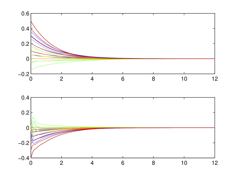
Remark 4

It should be noted that the proposed solution depends on the global information on the system topology. Specifically, the constants $\theta_{i}$ and $\sigma$ are determined by the communication topology (but do not depend on the interconnection topology). On the other hand, the LMIs (43) are setup using the knowledge of interconnection topology.

4 Example

To illustrate the proposed method, consider a mass-spring-damper system in Fig. 2. The system consists of $21$ identical masses which are coupled by different springs and dampers. Each mass is also connected to the wall with a spring. The dynamics of the coupled system are governed by the following equations

$$m\ddot{\alpha}_{0}= k_{1,1}(\alpha_{1}-\alpha_{0})+k_{1,2}(\dot{\alpha}_{1}-\dot{\alpha}_{0})+k_{0,1}(\alpha_{20}-\alpha_{0})+k_{0,2}(\dot{\alpha}_{20}-\dot{\alpha}_{0})-\bar{k}\alpha_{0},$$

$$m\ddot{\alpha}_{i}= k_{i,1}(\alpha_{i-1}-\alpha_{i})+k_{i,2}(\dot{\alpha}_{i-1}-\dot{\alpha}_{i})$$

$$+k_{i+1,1}(\alpha_{i+1}-\alpha_{i})+k_{i+1,2}(\dot{\alpha}_{i+1}-\dot{\alpha}_{i})-\bar{k}\alpha_{i}+u_{i},\quad i=1,\ldots,19,$$ (110)

$$m\ddot{\alpha}_{20}= k_{20,1}(\alpha_{19}-\alpha_{20})+k_{20,2}(\dot{\alpha}_{19}-\dot{\alpha}_{20})+k_{0,1}(\alpha_{0}-\alpha_{20})+k_{0,2}(\dot{\alpha}_{0}-\dot{\alpha}_{20})-\bar{k}\alpha_{20}+u_{20},$$

where $\alpha_{i}$, $\dot{\alpha}_{i}$ are the displacement and the velocity of mass $i$, $\bar{k}$ and $k_{i,1}$, $i=0,\ldots,20$ are the spring constants, $k_{i,2}$, $i=0,\ldots,20$ are the damper coefficients, and $m$ is the mass of each block.

Choosing the state vectors as $x_{i}=(\alpha_{i},\dot{\alpha}_{i}),i=0,\ldots,20$, each equation in (4) can be written in the form of (5), (6), where

$$A=\left[\begin{array}[]{cc}0&1\\ -\frac{\bar{k}}{m}&0\end{array}\right],\quad B_{1}=\left[\begin{array}[]{c}0\\ \frac{1}{m}\end{array}\right],\quad B_{2}=\left[\begin{array}[]{c}0\\ \frac{1}{m}\end{array}\right],$$

$$\varphi_{i,i-1}(z)=\varphi_{i-1,i}(z)=[k_{i,1}~{}k_{i,2}]z,\quad(i=1,\ldots,20)$$

$$\varphi_{0,20}(z)=\varphi_{20,0}(z)=[k_{0,1}~{}k_{0,2}]z,\quad z\in\mathbf{R}^{2}.$$

To verify the norm-bounded condition, let us assume that

$$[k_{i,1}~{}k_{i,2}]=\Delta_{i,i-1}C_{i,i-1},\quad[k_{0,1}~{}k_{0,2}]=\Delta_{0,20}C_{0,20},$$

where $C_{i,i-1}=[k_{i,1}~{}k_{i,2}]$, $C_{0,20}=[k_{0,1}~{}k_{0,2}]$, are given matrices, and $\Delta_{i,i-1}$, $\Delta_{0,20}\in[0,1]$ are scalars. Then all the couplings between the agents satisfy the norm bound condition (4). In this example, for simplicity we let $k_{i,1}=k_{i,2}=k$ for all $i=0,\ldots,20$.

The structure of the system (4) suggests that the agents are coupled according to the undirected cyclic graph shown in Fig. 3, since the force exerted by mass $i$ on mass $i+1$ exactly reciprocates the force exerted by mass $i+1$ on mass $i$:

$$k_{i+1,1}(\alpha_{i+1}-\alpha_{i})+k_{i+1,2}(\dot{\alpha}_{i+1}-\dot{\alpha}_{i})=-k_{i+1,1}(\alpha_{i}-\alpha_{i+1})-k_{i+1,2}(\dot{\alpha}_{i}-\dot{\alpha}_{i+1}).$$

We will treat the graph in Fig. 3 as a special case of directed graph with symmetric adjacency matrix. On the other hand, the communication topology of the system is assumed to be a directed graph shown in Fig 4. According to this graph, agents $1$, $8$, $12$ and $15$ observe the leader.

Figure 2: Mass-spring-damper system.

Figure 3: Undirected coupling graph.

Figure 4: Directed communication graph.

To illustrate the results of the paper, the protocol matrices were computed using Theorem 2, and then the trajectories of the coupled mass-spring-damper system with the obtained protocol were simulated. To design the protocol, the parameters of the coupled mass-spring-damper system were chosen to be $m=3$ kg, $k=0.1$ N/m, and $\bar{k}=2.4-1.4\rho(t)$ N/m with $\rho(t)=\cos(t)$. The headway distance between the mass bodies was assumed to be $1$ m.

In the simulation, the spring constants and damper coefficients were chosen to be $k_{i,1}=0.1$ N/m and $k_{i,2}=0.1$ N/(m/s), $i=0,\ldots,20$, respectively. The initial states of the leader and the followers were set to the values shown in table 1. In the cost function, we chose $Q=\begin{bmatrix}10&0\\ 0&100\end{bmatrix}$ and $R=0.001$.

Table 1: The initial states of the leader and followers.

$x_{0}^{\prime}(0)$	$x_{1}^{\prime}(0)$	$x_{2}^{\prime}(0)$	$x_{3}^{\prime}(0)$	$x_{4}^{\prime}(0)$	$x_{5}^{\prime}(0)$	$x_{6}^{\prime}(0)$
[0.5 0]	[0.45 0]	[0.4 0]	[0.3 0]	[0.2 0]	[0.15 0]	[0.25 0]
$x_{7}^{\prime}(0)$	$x_{8}^{\prime}(0)$	$x_{9}^{\prime}(0)$	$x_{10}^{\prime}(0)$	$x_{11}^{\prime}(0)$	$x_{12}^{\prime}(0)$	$x_{13}^{\prime}(0)$
[0.35 0]	[0.45 0]	[0.55 0]	[0.65 0]	[0.55 0]	[0.45 0]	[0.35 0]
$x_{14}^{\prime}(0)$	$x_{15}^{\prime}(0)$	$x_{16}^{\prime}(0)$	$x_{17}^{\prime}(0)$	$x_{18}^{\prime}(0)$	$x_{19}^{\prime}(0)$	$x_{20}^{\prime}(0)$
[0.45 0]	[0.5 0]	[0.4 0]	[0.3 0.1]	[0.2 0.2]	[0.1 0.3]	[0 0.4]

To design the synchronization protocol, we chose $\Gamma=[-1,1]$ with $4$ design points

$$\Gamma_{\ell}=\big{\{}-1,-0.3333,0.3333,1\big{\}}.$$

Choosing $\beta_{s}=0.3111$ so that the properties (62) hold for each design point, we solved the corresponding LMIs (43). Next, we constructed a continuous-gain control protocol by using the interpolation technique based on Theorem 2. We computed $\eta=0.0143$, $\varrho=0.0082$ and we need to select $q\in(0,1)$ such that $\sup_{t}|\dot{\rho}(t)|\leq 1.7485q$, $q\in(0,1)$. Since $\sup_{t}|\dot{\rho}(t)|=\sup_{t}|-\sin t|=1$, this allows us to choose $q=0.5750$. Then the theoretically predicted bound on the performance (85) is computed to be $329.1316$. On the other hand, by simulating the system on the time interval $[0,12]$, we numerically found the value of the performance cost (7) for this particular instance of the system to be equal to $\mathcal{J}(u)=39.7982$.

Moreover, switching control protocol which does not involve the interpolation technique was simulated in the example to compare difference between the gain scheduling and switching design. The computed performance cost (7) for the switching control of the system is equal to $\mathcal{J}(u)=40.2858$. The simulation results are shown in Fig. 5, 6, 7, 8 and 9.

Figure 5: Relative displacement (the top figure) and relative velocities of the followers with respect to the leader.

Figure 6: The displacement (the top figure) and velocity trajectories of the leader and followers.

Figure 7: The relative distance between the blocks.

Figure 8: The continuous control signals (the top figure) and switching control signals of the followers.

Figure 9: Accelerations of the leader and the followers without control forces (the top figure), with continuous control forces and switching control forces (the bottom figure).

The Fig. 5 demonstrates that the proposed continuous protocol enables all the followers to synchronize to the leader. The displacement and velocity trajectories of each block are shown in Fig. 6. Fig. 7 shows relative distances between the blocks $\alpha_{i}-\alpha_{i-1}+h$, where $h=1$m is the headway distance. From the figure, the relative distances vary initially between $0.9$m and $1.1$m and remain positive. This indicates that collisions between the blocks were avoided. Fig. 8 confirms that the control signals are continuous for each follower by using the interpolation technique, while the switching control scheme leads to discontinuous control signals. This also causes accelerations of the subsystems to be continuous and discontinuous, respectively; see Fig. 9. Discontinuous accelerations are often undesirable in practical systems. We also notice that the accelerations exerted by the proposed controllers are of comparable value with the accelerations occurring in the control-free system (Fig. 9); this indicates that the controller gains have been tuned to acceptable values.

5 Conclusions

The paper has considered the leader-follower control problem for a parameter varying system with directed communication topology and linear uncertain coupling, subject to norm-bounded constraints. In contrast to many existing works, we assume that the leader is selected among the agents, and remains coupled to the rest of the system. Therefore, in a sense the problem under consideration has addressed synchronization in leaderless interconnected multi-agent systems. The main technical challenge has been to overcome the effects of physical interconnections.

For this problem, we have proposed a continuous gain-scheduled consensus-type control protocol which employs an interpolation technique. The sufficient condition for the synchronization of the system is obtained which guarantees a suboptimal bound on tracking performance. The condition is in the LMI form, and is numerically tractable, although it requires solving coupled LMIs.

6 Acknowledgements

This work was supported by the Australian Research Council under Discovery Projects funding scheme (projects DP0987369 and DP120102152).

References

• [1] J. S. Shamma (editor). Cooperative control of distributed multi-agent systems. Wiley, 2007.
• [2] S. E. Tuna. Synchronizing linear systems via partial-state coupling. Automatica 2008; 44(8):2179–2184.
• [3] S. E. Tuna. Conditions for synchronizability in arrays of coupled linear systems. IEEE Transactions on Automatic Control 2009; 54(10):2416–2420.
• [4] R. Olfati-Saber and R. M. Murray. Consensus problems in networks of agents with switching topology and time-delays. IEEE Transactions on Automatic Control 2004; 49(9):1520–1533.
• [5] R. Olfati-Saber, J. A. Fax, and R. M. Murray. Consensus and cooperation in networked multi-agent systems. Proceedings of the IEEE 2007; 95(1):215–233.
• [6] P. Wieland, R. Sepulchre, and F. Allgöwer. An internal model principle is necessary and sufficient for linear output synchronization. Automatica 2011; 47(5):1068–1074.
• [7] L. M. Pecora and T. L. Carroll. Synchronization in chaotic systems. Physical Review Letters 1990; 64(8):821–824.
• [8] H. F. Grip, T. Yang, A. Saberi, and A. A. Stoorvogel. Output synchronization for heterogeneous networks of non-introspective agents. Automatica 2012; 48(10):2444–2453.
• [9] D. D. Šiljak. Large-scale dynamic systems: Stability and structure. NY: North-Holland, New York, 1978.
• [10] H. R. Pota, G. X. Athanasius, V. Ugrinovskii, and L. Li. Control design for interconnected power systems with OLTCs via robust decentralized control. American Control Conference, Minneapolis, Minnesota, USA, 2006; 3469–3474.
• [11] D. D. Šiljak. Decentralized control of complex systems. MA: Academic Press, Boston, 1991.
• [12] J. S. Shamma. An overview of LPV systems. Control of Linear Parameter Varying Systems with Applications, J. Mohammadpour and C. Scherer (editors), Springer, 2012.
• [13] F. D. Bianchi, H. De Battista, and R. J. Mantz. Wind turbine control systems: principles, modelling and gain scheduling design. Springer, 2006.
• [14] K. Morrisse, G. Solimini, and U. Khan. Distributed control schemes for wind-farm power regulation. North American Power Symposium (NAPS), Champaign, IL, USA, 2012; 1–6.
• [15] G. S. Seyboth, G. S. Schmidt, and F. Allgöwer. Cooperative control of linear parameter-varying systems. American Control Conference, Montreal, CA, USA, 2012; 2407–2412.
• [16] Q. Liu, C. Hoffmann, and H. Werner. Distributed control of parameter-varying spatially interconnected systems using parameter-dependent Lyapunov functions. American Control Conference, Washington, DC, USA, 2013; 3278–3283.
• [17] Y. Cheng, V. Ugrinovskii, and G. Wen. Guaranteed cost tracking for uncertain coupled multi-agent systems using consensus over a directed graph. Australian Control Conference, Perth, Australia, 2013; 375–378. Also, see arXiv:1309.0365.
• [18] G. S. Seyboth, G. S. Schmidt, and F. Allgöwer. Output synchronization of linear parameter-varying systems via dynamic couplings. IEEE Conference Decision and Control, Maui, Hawaii, USA, 2012; 5128–5133.
• [19] V. Ugrinovskii. Gain-scheduled synchronization of parameter varying systems via relative Hsubscript𝐻H_{\infty} consensus with application to synchronization of uncertain bilinear systems. Automatica 2014; 50(11):2880–2887.
• [20] V. Ugrinovskii. Conditions for detectability in distributed consensus-based observer networks. IEEE Tran. Autom. Contr. 2013; 58:2659–2664.
• [21] M. Yoon, V. Ugrinovskii, and M. Pszczel. Gain-scheduling of minimax optimal state-feedback controllers for uncertain linear parametervarying systems. IEEE Transactions on Automatic Control 2007; 52(2):311–317.
• [22] L. Scardovi and R. Sepulchre. Synchronization in networks of identical linear systems. Automatica 2009; 45:2557–2562.
• [23] A. Jadbabaie, J. Lin, and S. A. Morse. Coordination of groups of mobile autonomous agents using nearest neighbor rules. IEEE Transactions on Automatic Control 2003; 48(6):988–1001.
• [24] W. Ren and E. Atkins. Distributed multi-vehicle coordinated control via local information exchange. Int. J. Robust Nonlinear Control 2007; 17:1002–1033.
• [25] Z. Li, Z. Duan, G. Chen, and L. Huang. Consensus of multiagent systems and synchronization of complex networks: a unified viewpoint. IEEE Trans. Circuits Syst. I, Reg. Papers 2010; 57(1):213- 1 7224.
• [26] Y. Hong, J. Hu, and L. Gao. Tracking control for multi-agent consensus with an active leader and variable topology. Automatica 2006; 42(7):1177–1182.
• [27] J. Hu and Y. Hong. Leader-following coordination of multi-agent systems with coupling time delays. Physical A 2007; 374(2):853–863.
• [28] H. W. Zhang, Frank L. Lewis, and Z. H. Qu. Lyapunov, adaptive, and optimal design techniques for cooperative systems on directed communication graphs. IEEE Transactions on Industrial Electronics 2012; 59(7):3026–3041.
• [29] D. J. Stilwell and W. J. Rugh. Interpolation of observer state feedback controllers for gain scheduling. IEEE Transactions on Automatic Control 1999; 44(6):1225–1229.