Two and Three-Qubits Geometry, Quaternionic and Octonionic Conformal Maps, and Intertwining Stereographic Projection

Abstract

In this paper the geometry of two and three-qubit states under local unitary groups is discussed. We first review the one qubit geometry and its relation with Riemannian sphere under the action of group $SU(2)$. We show that the quaternionic stereographic projection intertwines between local unitary group $SU(2)\otimes SU(2)$ and quaternionic Möbius transformation. The invariant term appearing in this operation is related to concurrence measure. Yet, there exists the same intertwining stereographic projection for much more global group $Sp(2)$, generalizing the familiar Bloch sphere in 2-level systems. Subsequently, we introduce octonionic stereographic projection and octonionic conformal map (or octonionic Möbius maps) for three-qubit states and find evidence that they may have invariant terms under local unitary operations which shows that both maps are entanglement sensitive.

PACs Index: 03.67.a 03.65.Ud

1 Introduction

There are relations between geometry and structure of spinors in various area of quantum information theory [1, 2, 3, 4, 5, 6, 7, 8, 9, 10]. The simplest quantum states involve qubits (two-level systems), including spin states of a spin $\frac{1}{2}$ particle, the polarization states of a photon, or the ground and excited state of an atom or ion. Single qubit have simple geometric picture, i.e. pure states can be identified with points on the surface of the Bloch sphere $S^{2}$ and mixed states identified with points inside the Bloch sphere. Therefore it is tempting to find geometric pictures for the higher dimension quantum states which resemble one qubit representation. Finding the set of the Bloch vector representation for N-level systems, generalizing the familiar Bloch vector in 2-level systems, seems to be nontrivial task [11, 12].

The relation between the Hopf fibration, single qubit and two-qubit states has been studied by Mosseri and Dandoloff [13] in quaternionic skew-field and subsequently have been generalized to three-qubit state based on octonions by Bernevig and Chen [14] . However, there is also one more reason to look for conformal maps. For two qubit states the concurrence measure appears explicitly in quaternionic stereographic projection which geometrically means that non-entangled states are mapped from $S^{7}$ onto a 2-dimensional planar subspace of the target space ${\mathbb{R}}^{4}$. On the other hand it was shown that third Hopf fibration is also entanglement sensitive for three qubit states [14].

However, it seems that there is also another geometrical approach to describe one two and three qubit states called Möbius transformation [15, 16]. As is typical in physics, the local properties are more immediately useful than the global properties, and the local unitary transformation is of great importance. Therefore in this paper, we pursue a different approach to study the geometrical structure of two and three-qubit states under a local unitary transformation [17]. We show that the quaternionic stereographic projection of two-qubit states intertwines between the local unitary $SU(2)\otimes SU(2)$ and corresponding quaternionic Möbius transformations [18, 19], which can be useful in theoretical physics such as quaternionic quantum mechanics [20], quantum conformal field theory [17, 18, 19, 20, 21] and quaternionic computations [22]. This generalizes our early work restricted to group $SO(2)\otimes SU(2)$ [15]. However the action of transformations that involve with non-commutative quaternionic skew-field on a spinor (living in quaternionic Hilbert spaces) is more complicated than the complex one. Roughly speaking one must distinguish between the left and right actions of a quaternionic transformations on a given state [23]. This anomalous property of quaternionic transformation lead us of defining the special quaternionic Möbius transformations. An additional goal of this work is to generalize all feature to three-qubit states. While the formulation is almost trivial task for two-qubit case, the problem is more involved in all features as we must cast the three qubit states in noncommutative and non-associative octonion skew-field. we will show that the construction of octonionic stereographic projection and Möbius transformation under local unitary group $SU(2)\otimes SU(2)\otimes SU(2)$ turns out to be possible and as in two-qubit case, both are entanglement sensitive [24, 25, 26, 27, 28, 29], i.e. there are terms that is invariant under local unitary transformation which is related to concurrence measure. In all of these construction, we will insist on commutativity of diagrams which any two compositions of maps starting at one point in the diagram and ending at another are equal. This will be entirely in the language of algebraic topology [30, 31, 32].

The paper is organized as follows. In section 2, we briefly summarize one-qubit geometry and conformal map in a commutative diagram and give an example for evolution of quantum system in the complex plane by Hadamard like transformation. In section 3, we extend the results of Ref [15] to general local and global transformation. In section 4, we introduce the basic geometrical structure together with basic background material, incorporating all information we need for characterization of three-qubit geometry. Formulation the octonionic stereographic projection and Möbius transformation under local unitary group $SU(2)\otimes SU(2)\otimes SU(2)$ is established in this section. The paper is ended with a brief conclusion and two appendices.

2 One-qubit geometry

Let ${\mathcal{H}}_{d}^{\mathbb{F}}$ be a $d$ dimensional Hilbert space in the field or skew-field $\mathbb{F}=\mathbb{C}$, $\mathbb{Q}$ or $\mathbb{O}$ where $\mathbb{C},\mathbb{Q}$ and $\mathbb{O}$ are complex, quaternion and octonion field (or skew-field) respectively. An arbitrary one-qubit pure state in the complex two dimensional Hilbert space ${\mathcal{H}}_{2}^{\mathbb{C}}$, is given by

$$|\psi\rangle=\alpha_{0}|0\rangle+\alpha_{1}|1\rangle\quad\quad,\quad|\alpha_{0}|^{2}+|\alpha_{1}|^{2}=1\quad\quad,\quad\alpha_{0},\alpha_{1}\in\mathbb{C}.$$ (2.1)

We summarize the results of Ref. [16] for one qubit pure state in a compact form as a commutative diagram

$$\begin{CD}{\mathcal{H}}_{2}^{\mathbb{C}}@>{\mathcal{P}}>{}>\mathbb{\widetilde{C}}\\ @V{A}V{}V@V{}V{\mathcal{F}_{{}_{A}}}V\\ {\mathcal{H}}_{2}^{\mathbb{C}}@>{}>{\mathcal{P}}>\mathbb{\widetilde{C}}\end{CD}$$

where $\mathcal{P}$ denotes the stereographic projection for one-qubit state (2.1), i.e.

$$\mathcal{P}(|\psi\rangle):=\alpha_{0}\alpha_{1}^{-1}\in\mathbb{\widetilde{C}}=\mathbb{C}\cup\{\infty\},$$ (2.2)

and $\mathcal{F}_{{}_{A}}\in PSU(2)=SU(2)/\{\pm I\}$ is Möbius transformation corresponding to $2\times 2$ matrix $A\in SU(2)$ define as

$$A=\left(\begin{array}[]{cc}a&b\\ -\bar{b}&\bar{a}\end{array}\right)\ \longleftrightarrow\ \mathcal{F}_{{}_{A}}(z):=\frac{az+b}{-\bar{b}z+\bar{a}},\quad\quad|a|^{2}+|b|^{2}=1,\quad\quad a,b,z\in\mathbb{C}.$$ (2.3)

The Möbius transformations, generating the conformal group in the complex plane, can be identified with conformal transformations on the sphere using stereographic projection. Commutativity of the above diagram means that for any one-qubit state $|\psi\rangle$ and any $A\in SU(2)$ we have

$$\mathcal{F}_{{}_{A}}\mathcal{P}(|\psi\rangle)=\mathcal{P}(A|\psi\rangle).$$ (2.4)

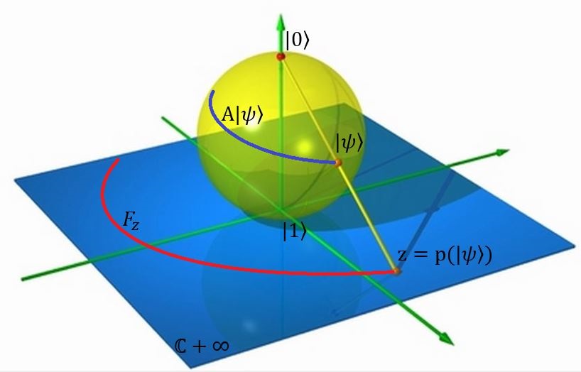
Figure 1: Stereographic map of Bloch sphere and time evolution of quantum states

This shows that the stereographic projection $\mathcal{P}$ intertwines between any single qubit unitary operation $A$ and it’s corresponding Möbius transformation $\mathcal{F}_{{}_{A}}$. The basic idea behind the stereographic projection $\mathcal{P}$ is easily to project the point on Bloch sphere (a pure quantum state) onto the point on the complex plain (see Fig. 1). The pure state (2.1) corresponds to the spin $\frac{1}{2}$ quantum states and it is well-known that it’s time evolution is governed by $2\times 2$ unitary matrices. For example, when we compare the states that differ by an exchange of coordinates on Riemannian sphere, we should, at least in principle, be able to tell by what unitary operation we effect this exchange for otherwise, we cannot really compare them other than in a formal and, in fact, in an ambiguous sense. According to Schrödinger equation $i\hbar\frac{\partial}{{\partial t}}\psi(x,t)=\mathcal{\hat{H}}\psi(x,t),$ all information about any quantum mechanical system is contained in the matrix elements of its time evolution operator

$$\psi(x,t)=e^{-i\mathcal{\hat{H}}t}\psi(x,0),$$ (2.5)

where $e^{-i\mathcal{\hat{H}}t}\equiv A\in SU(2)$, up to a global phase, describes dynamical evolution under the influence of the Hamiltonian from a time zero to time t. For example if we take the Hamiltonian as Hadamard gate

$$H=\frac{1}{{\sqrt{2}}}\left({\begin{array}[]{*{20}{c}}1&1\\ 1&{-1}\end{array}}\right),$$ (2.6)

and initial state as $|1\rangle$, then its time evolution on Bloch sphere reads

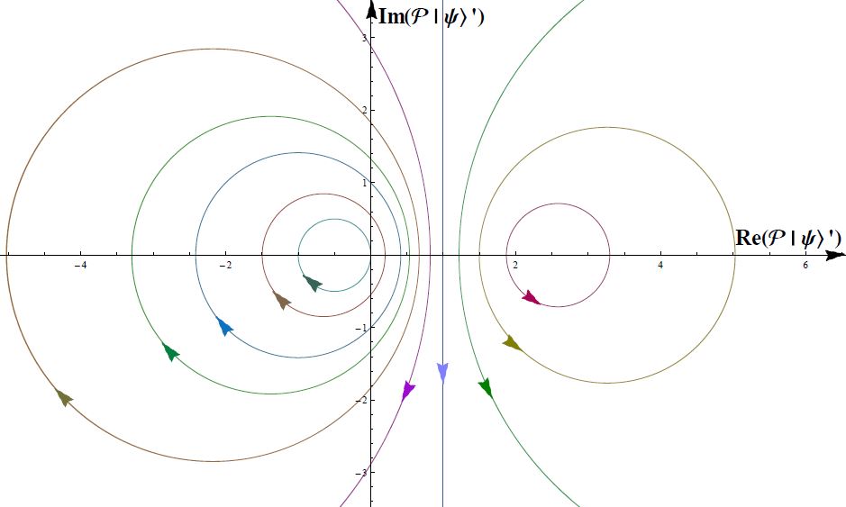
Figure 2: Time evolution of the state $(\cos\frac{\theta}{2}|0\rangle+e^{i\phi}\sin\frac{\theta}{2}|1\rangle)$ for various initial states with $\phi=0$ and $\theta=\frac{3}{15},\frac{4}{15},...,\frac{15}{15}$ by Hadamard like Hamiltonian.

$$|\psi(t)\rangle=e^{-iHt}|1\rangle=-\frac{i}{\sqrt{2}}\sin(t)|0\rangle+(\cos(t)+\frac{i}{\sqrt{2}}\sin(t))|1\rangle,$$ (2.7)

which in turn implies that its corresponding time dependent stereographic projection is

$$\mathcal{P}(e^{-iHt}|1\rangle)=\frac{-1}{2\cos^{2}(t)+\sin^{2}(t)}(\sin^{2}(t)+\sqrt{2}i\ \sin(t)\cos(t)),$$ (2.8)

(see Fig 3). On the other hand if we first map the initial state to complex plane $\mathcal{P}|1\rangle=0$ and then take its Möbius transformation

$$\mathcal{F}_{{}_{H}}(e^{-iHt}|1\rangle)=\frac{sin(t)}{\sqrt{2}i\ cos(t)-sin(t)},$$ (2.9)

which one can easily verified that it is equal to the right hand side of Eq. (2.8). An important geometrical property of Möbius transformation is that, they map circles onto circles as depicted in Fig (2). This also includes straight lines as circles of infinite radius. This result should not be too surprising: There is a group theoretical identity behind this observation, namely the isomorphism $SU(2)\simeq S^{2}\times U(1)$, where $U(1)$ is the gauge subgroup contained in $SU(2)$. Indeed, starting with any initial state and Hamiltonian yields the same result as above which come from the fact that the Möbius transformations preserve the angles (hence the name conformal).

3 Two-qubit geometry

It is tempting to try to extend the results of the last section to the system of bipartite two-qubit systems. However due to the difference between the dimensions of single qubit and two-qubit systems, there are a number mathematical differences which make the structure of the problem a much harder (but also more interesting!). Firstly, in one qubit quantum systems the state $\rho$ can be represented by its Bloch sphere representation, a vector $\vec{r}$ inside the unit ball in $\mathbb{R}^{3}$. The correspondance is given by

$$\rho=\frac{1}{2}(\mathbb{I}+\vec{r}.\vec{\sigma}),\quad\quad r_{i}=tr(\rho\sigma_{i}),$$ (3.10)

where $\mathbb{I}$ is identity matrix, $\{\sigma_{i}\}$ are the Pauli matrices and the geometry of state $\rho$ is completely described by the vector $\vec{r}$ on Bloch sphere such that, the points on the surface of the Bloch sphere correspond to the pure states of the system, whereas the interior points correspond to the mixed states. In general there is nothing like Bloch sphere representation for general two-qubit mixed states [11, 12] but rather one is dealing with a particular quaternionic representation for two-qubit pure states. Second, for two-qubit system there is a quantum correlation, i.e. entanglement which depends on locally or globally unitary transformation, therefore we must distinguish between local and global transformation.

3.1 Local unitary transformations

The Hilbert space ${\mathcal{H}}_{4}^{\mathbb{C}}$ of the compound system is the tensor product of the individual Hilbert spaces ${\mathcal{H}}_{2}^{\mathbb{C}}\otimes{\mathcal{H}}_{2}^{\mathbb{C}}$ with a direct product basis $\{|00\rangle,|01\rangle,|10\rangle,|11\rangle\}$. Any two-qubit pure state in this basis reads

$$|\psi\rangle=\alpha|00\rangle+\beta|01\rangle+\gamma|10\rangle+\delta|11\rangle\quad\quad\quad\alpha,\beta,\gamma,\delta,\in\mathbb{C},$$ (3.11)

with normalization condition $|\alpha|^{2}+|\beta|^{2}+|\gamma|^{2}+|\delta|^{2}=1$. We summarize the result of [15] in a commutative diagram fashion covenant for our purposes as

$$\begin{CD}{\mathcal{H}}_{4}^{\mathbb{C}}@>{\mathcal{Q}}>{}>{\mathcal{H}}_{2}^{\mathbb{Q}}@>{\mathcal{P}}>{}>\mathbb{\widetilde{Q}}\\ @V{B}V{}V@V{\mathbb{Q}B}V{}V@V{}V{\mathcal{F}_{{}_{B}}}V\\ {\mathcal{H}}_{4}^{\mathbb{C}}@>{\mathcal{Q}}>{}>{\mathcal{H}}_{2}^{\mathbb{Q}}@>{\mathcal{P}}>{}>\mathbb{\widetilde{Q}}\end{CD}$$

where $\mathcal{Q}$ denotes the quaternification operation which maps every $|\psi\rangle\in{\mathcal{H}}_{4}^{\mathbb{C}}$ to quaterbit $|{\psi}\rangle_{q}\in{\mathcal{H}}_{2}^{\mathbb{Q}}$ as follows

$$\mathcal{Q}(|\psi\rangle):=|{\psi}\rangle_{q}=q_{1}|{0}\rangle_{q}+q_{2}|{1}\rangle_{q}=\left(\begin{array}[]{c}q_{1}\\ q_{2}\\ \end{array}\right),\quad\quad|q_{1}|^{2}+|q_{2}|^{2}=1,$$ (3.12)

where $q_{1}=\alpha+\beta e_{2}$ and $q_{2}=\gamma+\delta e_{2}$ are quaternion numbers (see appendix A). Note that this map is bijective (one to one and onto). $\mathcal{P}$ is the quaternionic stereographic projection for quaterbit defined as

$$\mathcal{P}(|\psi\rangle_{q}):=q_{1}q^{-1}_{2}=\frac{1}{|q_{2}|^{2}}(S+Ce_{2})\in\mathbb{\widetilde{Q}}=\mathbb{Q}\cup\{\infty\},$$ (3.13)

where $S=\alpha\overline{\gamma}+\beta\overline{\delta}$ and $C=\beta\gamma-\alpha\delta$ are Schmidt and concurrence terms respectively. If $S=0$, then the two-qubit pure state have Schmidt form $(\sqrt{\lambda_{1}}|00\rangle+\sqrt{\lambda_{2}}|11\rangle)$ with positive numbers $\lambda_{1}$ and $\lambda_{2}$. On the other hand $2|C|$ is concurrence measure for two-qubit pure state meaning that if $C=0$ then the two qubit pure state (3.11) is reduced to a separable state, i.e. factorized as $|\psi\rangle_{AB}=|\psi\rangle_{A}|\psi\rangle_{B}$ [33]. This means that there is an one to one correspondence between the points on complex plane $\mathbb{\widetilde{C}}$ and two-qubit separable states. Let us mention that that the map $\mathcal{P}$ is related to the stereographic projection of the second Hopf fibration of the form

$$\mathcal{P}:\mathbb{Q}^{2}\xrightarrow{}\mathbb{Q}\mathbb{P}^{1},$$ (3.14)

where $\mathbb{Q}\mathbb{P}^{1}$ is the one dimensional quaternionic projective space. In this diagram $B\in SU(2)\otimes SU(2)$ is any local unitary transformation acting on two-qubit pure state (3.11)

$$|\psi\rangle^{\prime}=A\otimes A^{\prime}|\psi\rangle,\ \ \ \ A,A^{\prime}\in SU(2).$$ (3.15)

Remembering that, $SU(2)$ transformation can be parameterized in the complex field as

$$A=\left({\begin{array}[]{*{20}{c}}a&b\\ {-\bar{b}}&\bar{a}\end{array}}\right),\quad\quad|a^{2}|+|b^{2}|=1,$$ (3.16)

we may alternatively write the transformation (3.15) in quaternionic right module as follows

$$|{\psi}\rangle^{\prime}_{q}=\mathbb{Q}B(|{\psi}\rangle_{q}):=A|{\psi}\rangle_{q}{\mathcal{A}^{\prime}}^{(q)}=\left({\begin{array}[]{*{20}{c}}a&b\\ {-\bar{b}}&\bar{a}\end{array}}\right)\left(\begin{array}[]{c}q_{1}\\ q_{2}\end{array}\right)(a^{\prime}-\bar{b}^{\prime}e_{2}),$$ (3.17)

where

$${\mathcal{A}^{\prime}}^{(q)}=a^{\prime}-\bar{b}^{\prime}e_{2}$$ (3.18)

and the second equality by itself defines the $\mathbb{Q}B$ operation in the diagram. The definition ${\mathcal{A}^{\prime}}^{(q)}=a^{\prime}-\bar{b}^{\prime}e_{2}$ as quaternionic representation for unitary matrix $A^{\prime}$ come from the isomorphism $Sp(1)\simeq SU(2)$. Because of the associativity of quaternion numbers, there is no ambiguity when it comes to forming products of higher order, i.e. $(q_{1}q_{2})q_{3}=q_{1}(q_{2}q_{3})=q_{1}q_{2}q_{3}$. Finally, the quaternionic Möbius transformation $\mathcal{F}_{{}_{B}}$ associated to the local unitary transformation $B=A\otimes A^{\prime}\in SU(2)\otimes SU(2)$ is defined as

$$\mathcal{F}_{{}_{B}}(q):=[{{aq{\mathcal{A}^{\prime}}^{(q)}+b{\mathcal{A}^{\prime}}^{(q)}}}][{{-\bar{b}q{\mathcal{A}^{\prime}}^{(q)}+\bar{a}{\mathcal{A}^{\prime}}^{(q)}}}]^{-1}$$

$$\ \ \ \ \ \ \ \ \ =\frac{S^{\prime}+C^{\prime}e_{2}}{|q_{2}|^{2}|b|^{2}+|a|^{2}-2Re(\bar{b}q_{2}a)}$$ (3.19)

where $q=\mathcal{P}(|{\psi}\rangle_{q})$ is stereographic projection of the initial state (3.11) and $Re(q)=\frac{1}{2}(q+\bar{q})$ is a real part of quaternion number $q$ and $C^{\prime}=C=(\beta\gamma-\alpha\delta)$ is concurrence term which is invariant under local unitary operations, as one would expect, while

$$S^{\prime}=(|q_{2}|^{2}-|q_{1}|^{2})ab+S|a|^{2}-\bar{S}|b|^{2}$$ (3.20)

is Schmidt term which unlike the concurrence term is not invariant under local unitary groups, even if the initial two-qubit state (3.11) being in Schmidt form in the old basis, i.e. $S=0$. Summarizing, we have found that the quaternionic stereographic projection $\mathcal{P}$ intertwines between the unitary local operation $B$ and the corresponding quaternionic Möbius transformation $\mathcal{F}_{{}_{B}}$ viz.

$$\mathcal{P}\mathcal{Q}B|\psi\rangle=\mathcal{P}(\mathbb{Q}B)\mathcal{Q}|\psi\rangle=\mathcal{F}_{{}_{B}}\mathcal{P}\mathcal{Q}|\psi\rangle.$$ (3.21)

It should be mentioned that $\mathcal{Q}B$ acting on quaterbit $|\psi\rangle_{q}$, endowed with right module as Eq. (3.17), belongs to the general form of local unitary transformation and there was no need to do with restriction $SO(2)\otimes SU(2)$ or $SU(2)\otimes SO(2)$ as established in Ref. [15] which, in turn, implies that the imaginary part of stereographic projection (3.13) is also an entanglement measure for two-qubit pure states.

3.2 Global unitary transformations Sp(2)

In deriving the result (3.21) we have restricted ourselves to the discussion of local unitary transformations. For less restrictive geometry we consider quaternionic spinor $|\psi\rangle_{q}=q_{1}|0\rangle_{q}+q_{2}|1\rangle_{q}$ and demand its transformation under global unitary transformations $Sp(2)$, the quaternionic counterpart of group $SU(2)$, which is defined as

$$Sp(2):=\{A\in GL(2,\mathbb{Q}):A^{\dagger}A=I\},$$ (3.22)

or equivalently it can be expressed as

$$Sp(2):=\{U\in U(4):UJU^{T}=J\},$$ (3.23)

where $J=I\otimes(-i\sigma_{2})$ and $\sigma_{2}$ is usual second Pauli matrix. If we define the action of every element of $Sp(2)$ on quaternionic spinor as

$$|\psi\rangle^{\prime}_{q}=A|\psi\rangle_{q}=\left(\begin{array}[]{cc}p_{1}&p_{2}\\ p_{3}&p_{4}\\ \end{array}\right)\left(\begin{array}[]{c}q_{1}\\ q_{2}\\ \end{array}\right)=\left(\begin{array}[]{c}p_{1}q_{1}+p_{2}q_{2}\\ p_{3}q_{1}+p_{4}q_{2}\\ \end{array}\right),$$ (3.24)

and its corresponding Möbius transformation as follows

$$\mathcal{F}_{{{}_{A}}}(q)=[p_{1}q+p_{2}][p_{3}q+p_{4}]^{-1},$$ (3.25)

with all $p_{i},q_{i}\in\mathbb{Q}$ being quaternionic number, then the stereographic projection (3.13) intertwines between $Sp(2)$ and Möbius transformation, i.e. $\mathcal{P}(A|\psi\rangle)=\mathcal{F}_{{}_{A}}\mathcal{P}|\psi\rangle$. Written more explicitly,

$$\mathcal{P}(Sp(2)|\psi\rangle_{q})=\mathcal{F}_{{}_{Sp(2)}}(\mathcal{P}|\psi\rangle_{q})=\frac{(|q_{1}|^{2}p_{1}\bar{p}_{3}+p_{1}q_{1}\bar{q}_{2}\bar{q}_{4}+p_{2}q_{2}\bar{q}_{1}\bar{q}_{3}+|q_{2}|^{2}p_{2}\bar{p}_{4})}{|p_{3}q_{1}+p_{4}q_{2}|^{2}},$$ (3.26)

or in the diagrammatic form actually reads

$$\begin{CD}{\mathcal{H}}_{2}^{\mathbb{Q}}@>{\mathcal{P}}>{}>\mathbb{\widetilde{Q}}\\ @V{Sp(2)}V{}V@V{}V{\mathcal{F}_{{}_{Sp(2)}}}V\\ {\mathcal{H}}_{2}^{\mathbb{Q}}@>{}>{\mathcal{P}}>\mathbb{\widetilde{Q}}\end{CD}$$

The derivation made here is based on explicit use of the particular form of Möbius transformation (3.25) and as in the case of local unitary transformation it is unique. The description above, albeit perfectly valid, still suffers from a deficiency: There is two-qubit state representation, like as Eq. (3.11), for quaternionic spinor but the first equality in Eq. (3.21) diagram does not hold for quaternionic spinor and the discussion may have seemed somewhat abstract. Nonetheless, the derivation is instructive and helps to understand the algebraic topology of quaternionic spinors (see, e.g. [32]).

4 Geometry of three-qubit states under local unitary groups

This section devoted to provide some basic tools and background to describe the geometry of three-qubit pure states under local unitary transformations.

4.1 Octonionic conformal map

The Hilbert space ${\mathcal{H}}_{8}^{\mathbb{C}}$ for three-qubit system is the tensor product of the individual Hilbert spaces ${\mathcal{H}}_{2}^{\mathbb{C}}\otimes{\mathcal{H}}_{2}^{\mathbb{C}}\otimes{\mathcal{H}}_{2}^{\mathbb{C}}$ with a direct product basis $\{|000\rangle,|001\rangle,|010\rangle,011\rangle,|100\rangle,|101\rangle,|110\rangle,|111\rangle\}$. An arbitrary three-qubit pure state in this basis read as

$$|\psi\rangle=t_{0}|000\rangle+t_{1}|001\rangle+t_{2}|010\rangle+t_{3}|011\rangle+t_{4}|100\rangle+t_{5}|101\rangle+t_{6}|110\rangle+t_{7}|111\rangle,$$ (4.27)

where $t_{i}\in\mathbb{C}$ are complex numbers and satisfy the normalization condition $\sum_{i=0}^{7}|t_{i}|^{2}=1$. Once again, projecting onto a basis in which all coefficients are singly quaternionic number, we can equivalently rewrite every $|\psi\rangle\in{\mathcal{H}}_{8}^{\mathbb{C}}$ by two-quaterbit $|{\psi}\rangle_{q}\in{\mathcal{H}}_{4}^{\mathbb{Q}}$ as

$$\mathcal{Q}(|\psi\rangle):=|{\psi}\rangle_{q}=q_{1}|{00}\rangle_{q}+q_{2}|{01}\rangle_{q}+q_{3}|{10}\rangle_{q}+q_{4}|{11}\rangle_{q}$$ (4.28)

where

$$q_{1}=t_{0}+t_{1}e_{2}\quad,q_{2}=t_{2}+t_{3}e_{2}\quad,q_{3}=t_{4}+t_{5}e_{2}\quad,q_{4}=t_{6}+t_{7}e_{2},\quad$$ (4.29)

and $\sum_{i=1}^{4}|q_{i}|^{2}=1$, is normalization condition in the language of quaternion numbers. By a straightforward rearrangement of the quaternion numbers, this can be rewritten as

$$|{\psi}\rangle_{o}=\mathcal{O}(\mathcal{Q}(|\psi\rangle))=\mathcal{O}|{\psi}\rangle_{q}=o_{1}|{0}\rangle_{o}+o_{2}|{1}\rangle_{o},$$ (4.30)

where $o_{1}=q_{1}+q_{2}e_{4}$ and $o_{2}=q_{3}+q_{4}e_{4}$ are octonion numbers (see Appendix A). Clearly, $|{\psi}\rangle_{o}$ is an octonion bit (octobit) which belongs to the Hilbert space ${\mathcal{H}}_{2}^{\mathbb{O}}$. Consider now a general octonion number

$$o=x_{0}e_{0}+x_{1}e_{1}+x_{2}e_{2}+x_{3}e_{3}+x_{4}e_{4}+x_{5}e_{5}+x_{6}e_{6}+x_{7}e_{7},\quad x_{i}\in\mathbb{R},$$ (4.31)

with inverse $o^{-1}=\frac{1}{|o|^{2}}\bar{o}$ where $\bar{o}$ is the complex conjugate of octonion $o$ defined as

$$\bar{o}=x_{0}e_{0}-x_{1}e_{1}-x_{2}e_{2}-x_{3}e_{3}-x_{4}e_{4}-x_{5}e_{5}-x_{6}e_{6}-x_{7}e_{7}.$$ (4.32)

Another definition which is necessary to formulate the octonionic stereographic projection is to define $\tilde{o}$ as

$$\tilde{o}=x_{0}e_{0}+x_{1}e_{1}+x_{2}e_{2}+x_{3}e_{3}+x_{4}e_{4}+x_{5}e_{5}+x_{6}e_{6}-x_{7}e_{7}.$$ (4.33)

Using the above definition and Eq. (4.30) and (4.32), the octonionic stereographic projection $\mathcal{P}$ is defined [13, 14]

$$\mathcal{P}(|{\psi}\rangle_{o}):=\tilde{o}_{1}\tilde{o}^{-1}_{2}=\frac{1}{|o_{2}|^{2}}(S_{0}+S_{1}e_{2}+(S_{2}+S_{3}e_{2})e_{4})\in\mathbb{\widetilde{O}}=\mathbb{O}\cup\{\infty\},$$ (4.34)

where

$$\begin{array}[]{c}{S_{0}}=t_{0}\bar{t_{4}}+t_{1}\bar{t_{5}}+t_{2}\bar{t_{6}}+t_{3}\bar{t_{7}},\\ {S_{1}}=t_{1}t_{4}-t_{0}t_{5}+\bar{t_{3}}\bar{t_{6}}-\bar{t_{2}}\bar{t_{7}},\\ {S_{2}}=t_{2}t_{4}-t_{0}t_{6}+\bar{t_{1}}\bar{t_{7}}-\bar{t_{3}}\bar{t_{5}},\\ {S_{3}}=t_{2}t_{5}-t_{1}t_{6}+\bar{t_{3}}\bar{t_{4}}-\bar{t_{0}}\bar{t_{7}},\end{array}$$ (4.39)

and $|\tilde{o}_{2}|^{2}=|o_{2}|^{2}=|t_{4}|^{2}+|t_{5}|^{2}+|t_{6}|^{2}+|t_{7}|^{2}$. An alternative, and often more useful representation of $\tilde{o}_{1}$ and $\tilde{o}_{2}$ is given by

$$\begin{array}[]{c}\tilde{o}_{1}=t_{0}+t_{1}e_{2}+(t_{2}+{\bar{t}}_{3}e_{2})e_{4},\\ \tilde{o}_{2}=t_{4}+t_{5}e_{2}+(t_{6}+{\bar{t}}_{7}e_{2})e_{4}.\end{array}$$ (4.42)

Note that, due to the non-associativity of octonions, i.e. $o_{1}(o_{2}o_{3})\neq(o_{1}o_{2})o_{3}$ one must keep the parenthesis in all equations involving the product of three or more octonions. The octonionic stereographic projection $\mathcal{P}$ is related to the stereographic projection of the third Hopf fibration of the form

$$\mathcal{P}:\mathbb{O}^{2}\xrightarrow{}\mathbb{O}\mathbb{P}^{1},$$ (4.43)

where $\mathbb{O}\mathbb{P}^{1}$ is the one dimensional octonionic projective space. An important characteristic of the stereographic projection (4.34), (or third Hopf fibration in [13, 14]), is its sensitivity to entanglement. To give it a more concrete meaning, we must express the entanglement of three-qubit state (4.27) in terms of concurrence measure introduced by Akhtarshenas [34]. To this end we assume general form of bipartite pure state

$$\left|\psi\right\rangle_{AB}=\sum\limits_{i=1}^{N_{1}}{\sum\limits_{j=1}^{N_{2}}{a_{ij}\left|{i\rangle\otimes|j}\right\rangle}},$$ (4.44)

which the norm of concurrence vector in terms of the $a_{ij}$ reads as

$$C^{AB}=2\sqrt{\sum\limits_{i<j}^{N_{1}}{\sum\limits_{k<l}^{N_{2}}{\left|{a_{ik}a_{jl}-a_{il}a_{jk}}\right|^{2}}}},$$ (4.45)

If we take the first qubit as partition $A$ and the last two qubits as partition $B$ in three-qubit state (4.27), then its concurrence can be calculated in terms of coefficients $t_{i}$ as

$$\begin{array}[]{l}C^{1(23)}=2(|t_{0}t_{5}-t_{1}t_{4}|^{2}+|t_{0}t_{6}-t_{2}t_{4}|^{2}+|t_{0}t_{7}-t_{3}t_{4}|^{2}\\ \quad\quad\quad\quad+|t_{1}t_{6}-t_{2}t_{5}|^{2}+|t_{1}t_{7}-t_{3}t_{5}|^{2}+|t_{2}t_{7}-t_{3}t_{6}|^{2})^{\frac{1}{2}}.\end{array}$$ (4.46)

Now if $C^{1(23)}=0$, i.e. first qubit is factorized from the last two qubits, then the terms $S_{1},S_{2}$ and $S_{3}$ in stereographic projection (4.34) vanish meaning that the separable states is projected to complex plane. Note that the inverse of this statement is not true, i.e. there are points on complex plane that have no separable counterpart at all.

Following the same logic as marshalled in section 2 for two-qubit states, we consider the general form of local unitary transformation that act on three-qubit state (4.27) as

$$|\psi\rangle\to|\psi\rangle^{\prime}={A_{1}}\otimes{A_{2}}\otimes{A_{3}}|\psi\rangle.$$ (4.47)

where all ${A_{i}}$ belong to the group $SU(2)$ and they can be parameterized as

$${A_{i}}=\left({\begin{array}[]{*{20}{c}}{{a_{i}}}&{{b_{i}}}\\ {-{{\bar{b}}_{i}}}&{{{\bar{a}}_{i}}}\end{array}}\right),\quad\quad|a_{i}|^{2}+|b_{i}|^{2}=1\ .$$ (4.48)

Writing three-qubit state (4.27) in the aforementioned quaternion and octonion forms in Eqs. (4.28) and (4.30), we can perform local unitary transformation as follows

$$|\psi\rangle^{\prime}_{q}={A_{1}}\otimes{A_{2}}[|\psi\rangle_{q}\mathcal{A}_{3}^{(q)}]={A_{1}}\otimes{A_{2}}[|\psi\rangle_{q}(a_{3}-\bar{b}_{3}e_{2})],$$ (4.49)

$$|\psi\rangle^{\prime}_{o}={A_{1}}\{[|\psi\rangle_{o}(\mathcal{A}_{3}^{(q)})](\mathcal{A}_{2}^{(o)})\},$$ (4.50)

where the octonionic representation $\mathcal{A}_{2}^{(o)}=a_{2}-\bar{b}_{2}e_{4}$ is defined analogous to Eq. (3.18) except that $e_{2}$ is replaced by $e_{4}$. We now make the octonionic stereographic projection which includes the local unitary groups as

$$\mathcal{P}((|{\psi}\rangle^{\prime}_{o})=\frac{1}{|o^{\prime}_{2}|^{2}}\frac{(a_{1}\tilde{o}_{1}+b_{1}\tilde{o}_{2})([\mathcal{A}_{3}^{(q)}\{\mathcal{A}_{2}^{(o)}\bar{\mathcal{A}}_{2}^{(o)}\}\bar{\mathcal{A}}_{3}^{(q)}])(-\bar{\tilde{o}}_{1}b+\bar{\tilde{o}}_{2}a)}{|(-\bar{b_{1}}[\{{\tilde{o}}_{1}\mathcal{A}_{3}^{(q)}\}\mathcal{A}_{2}^{(o)}])+(\bar{a}_{1}[\{\tilde{o}_{2}(\mathcal{A}_{3}^{(q)}\}\mathcal{A}_{2}^{(o)}])|^{2}},$$ (4.51)

where $o^{\prime}_{2}=-\bar{b}_{1}[\{o_{1}\mathcal{A}_{3}^{(q)}\}\mathcal{A}_{2}^{(o)}]+\bar{a}_{1}[\{o_{2}\mathcal{A}_{3}^{(q)}\}\mathcal{A}_{2}^{(o)}]$. The definition (4.51) reduces to Eq. (4.34), whenever we take $A_{1},A_{2}$ and $A_{3}$ as identity operator $I$.

Finally, we define the octonionic Möbius transformations as

$$\mathcal{F}_{{}_{B}}(o):=\frac{(a_{1}o+b_{1})([\mathcal{A}_{3}^{(q)}\{\mathcal{A}_{2}^{(o)}\bar{\mathcal{A}}_{2}^{(o)}\}\bar{\mathcal{A}}_{3}^{(q)}])(-\bar{o}b+a)}{|-\bar{b}_{1}[\{o\mathcal{A}_{3}^{(q)}\}\mathcal{A}_{2}^{(o)}]+\bar{a}_{1}\{\mathcal{A}_{3}^{(q)}\mathcal{A}_{2}^{(o)}\}|^{2}},$$ (4.52)

where $o=\mathcal{P}(|{\psi}\rangle_{o})$ is stereographic projection of the initial state (4.27). This unique choice of octonionic Möbius transformation is based on the implicit fact that we treat the space of octonionic spinors as a right module (multiplication by quaternions and octonions from the right). Regarding above considerations, we finally state our main result in the commutative diagram as

$$\begin{CD}{\mathcal{H}}_{8}^{\mathbb{C}}@>{\mathcal{Q}}>{}>{\mathcal{H}}_{4}^{\mathbb{Q}}@>{\mathcal{O}}>{}>{\mathcal{H}}_{2}^{\mathbb{O}}@>{\mathcal{P}}>{}>\mathbb{\widetilde{O}}\\ @V{B}V{}V@V{}V{\mathbb{Q}B}V@V{}V{\mathbb{O}B}V@V{}V{\mathcal{F}_{{}_{B}}}V\\ {\mathcal{H}}_{8}^{\mathbb{C}}@>{\mathcal{Q}}>{}>{\mathcal{H}}_{4}^{\mathbb{Q}}@>{\mathcal{O}}>{}>{\mathcal{H}}_{2}^{\mathbb{O}}@>{\mathcal{P}}>{}>\mathbb{\widetilde{O}}\end{CD}$$

In the present case commutativity of the diagram is equivalent to the commutativity relation (for more detail see Appendix B)

$$\mathcal{P}\mathcal{O}\mathcal{Q}(B)|\psi\rangle=\mathcal{P}\mathcal{O}(\mathbb{Q}B)\mathcal{Q}|\psi\rangle=\mathcal{P}(\mathbb{O}B)\mathcal{O}\mathcal{Q}|\psi\rangle=\mathcal{F}_{{}_{B}}\mathcal{P}\mathcal{O}\mathcal{Q}|\psi\rangle,$$ (4.53)

Before concluding this section, let us make some preliminary remarks on the general properties of this diagram. As it is evident from the last equality, we have $\mathcal{P}(\mathbb{O}B)|\psi\rangle_{o}=\mathcal{F}_{{}_{B}}\mathcal{P}|\psi\rangle_{o},$ i.e. the octonion stereographic projection $\mathcal{P}$ intertwines between $(\mathbb{O}B)$ and octonionic Möbius transformation $\mathcal{F}_{{}_{B}}$. As mentioned earlier in this section, the terms $S_{1},S_{2}$ and $S_{3}$ are entanglement sensitive, therefore we expect that they become invariant under local unitary transformations, i.e. $S^{\prime}_{i}=S_{i}$ hold for $i=1,2,3$ (for aprecise proof, see Appendix B).

5 Conclusion

In summary, we have considered some geometrical aspects of one, two and three-qubit pure states under local unitary transformation. In this investigation we saw that the stereographic projection $\mathcal{P}$ plays a crucial role. For one-qubit states, the mapping is one to one correspondence between Bloch sphere and complex projective space $\mathbb{\widetilde{C}}$. In addition, $\mathcal{P}$ intertwines between unitary group $SU(2)$ and its corresponding complex Möbius transformation. As an example we have discussed the time evolution of one-qubit state under Hadamard like Hamiltonian in more detail. Considering two-qubit states we observe the following features: A rather generalized intertwining stereographic projection $\mathcal{P}$, between global group $Sp(2)$ and its corresponding quaternionic Möbius transformation, is easy to construct, but in general it is not completely equivalent to work with the two-qubit states due to the non-commutativity of quaternion numbers in its definition. However, for local unitary transformation $SU(2)\otimes SU(2)$ there is unique quaternionic stereographic projection $\mathcal{P}$ and Möbius transformation, both leave the concurrence term invariant and fulfill the Eq. (3.21), i.e. we have a commuting diagram. The geometry of the three-qubit is generally richer than that of two-qubit states. More generally, the octonionic representation of three-qubit states cannot be transformed under a global group which places it outside the line of treatments of one and two-qubit cases. This is due to the fact that, octonion numbers are not only noncommutative but also they are non-associative. For a different task, however, the construction of octonionic stereographic projection $\mathcal{P}$ and Möbius transformation under local unitary group turns out to be possible. As in the case of two-qubits, both octonionic stereographic projection and Möbius transformation are entanglement sensitive, i.e. there are terms that is invariant under local unitary transformation $SU(2)\otimes SU(2)\otimes SU(2)$ and have something to do with concurrence measure. In all of these construction, we have insisted on commutativity of diagrams.

Appendix A: Quaternion and Octonion
The quaternion skew-field $\mathbb{Q}$ is an associative algebra of rank 4 on real number $\mathbb{R}$ whose every element can be written as

$$q=\sum\limits_{i=0}^{3}{{x_{i}}{e_{i}}},\quad\quad{x_{i}}\in\mathbb{R},$$ (A-1)

where $e_{0}=1$ and $e_{1},e_{2},e_{3}$ satisfy

$$e_{1}^{2}=e_{2}^{2}=e_{3}^{2}=-1,\quad e_{1}e_{2}=-e_{2}e_{1}=e_{3},\quad e_{2}e_{3}=-e_{3}e_{2}=e_{1},\quad e_{3}e_{1}=-e_{1}e_{3}=e_{2}.$$ (A-2)

It can also be defined equivalently, using the complex numbers $z_{1}=x_{0}+x_{1}e_{1}$ and $z_{2}=x_{2}+x_{3}e_{1}$ in the form $q=z_{1}+z_{2}e_{2}$ endowed with an involutory anti-automorphism (conjugation) such as

$$q=z_{1}+z_{2}e_{2}\in\mathbb{C}\oplus\mathbb{C}e_{2}\ \longrightarrow\ \bar{q}=x_{0}-\sum\limits_{i=1}^{3}{{x_{i}}{e_{i}}}=\bar{z}_{1}-z_{2}e_{2}.$$ (A-3)

Note that quaternion multiplication is non-commutative so that $\overline{q_{1}q_{2}}={\overline{q_{2}}}\ {\overline{q_{1}}}$ and $e_{2}z=\bar{z}e_{2}$. On the other hand a two dimensional quaternionic vector space $V$ defines a four dimensional complex vector space $\mathbb{C}V$ by forgetting scalar multiplication by non-complex quaternions (i.e., those involving $e_{2}$). Roughly speaking if $V$ has quaternionic dimension $2$, with basis $|0\rangle_{q},|1\rangle_{q}$, then $\mathbb{C}V$ has complex dimension 4, with basis $\{|00\rangle,|01\rangle,|10\rangle,|11\rangle\}$.

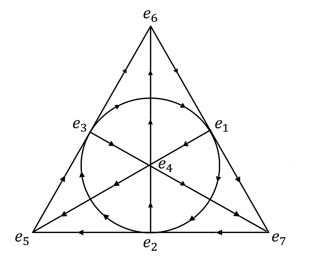
Figure 3: Multiplication rule for octonion.

The octonionic skew-field $\mathbb{O}$ is neither commutative nor associative algebra of rank 8 over $\mathbb{R}$ whose every element can be written as

$$o=\sum\limits_{i=0}^{7}{{x_{i}}{e_{i}}}\quad\quad,{x_{i}}\in\mathbb{R}\quad\quad,{e_{0}}=1\quad\mathrm{and}\quad e_{i}^{2}=-1{\kern 1.0pt}{\kern 1.0pt}(i=1,...,7).$$ (A-4)

The multiplication of octonion is given by

$${e_{i}}{e_{j}}=-{\delta_{ij}}{e_{0}}+\sum\limits_{k=1}^{7}{{f_{ijk}}{e_{k}}}\quad\quad\mathrm{for}\quad\quad i,j=1,2,...,7\ \ ,$$ (A-5)

where the ${f_{ijk}}$ are totally anti-symmetric in $i,j$ and $k$ with values $1,0,-1$ just as Levi-Civita symbol. Moreover, $f_{ijk}=+1$ for $ijk=123,145,246,347,617,725,536$. We can depict this fact graphically as in (Fig. 3) where the multiplication role can be read from orientation of arrows, for example:

$$e_{1}e_{2}=e_{3},\quad\quad e_{2}e_{4}=e_{6},\quad\quad e_{7}e_{2}=e_{5}.$$ (A-6)

The complex conjugate of a octonion is given by

$$\bar{o}=x_{0}-\sum\limits_{i=1}^{7}{{x_{i}}{e_{i}}}.$$ (A-7)

Any octonion number can be represented in terms of four complex number $z_{0}=x_{0}+x_{1}e_{1}$, $z_{1}=x_{2}+x_{3}e_{1}$, $z_{2}=x_{4}+x_{5}e_{1}$ and $z_{3}=x_{6}+x_{7}e_{1}$ as

$$o=z_{0}+z_{1}e_{2}+(z_{3}+z_{3}e_{2})e_{4},$$ (A-8)

and it’s complex conjugate is given by

$$\bar{o}=\bar{z}_{0}-z_{1}e_{2}-(z_{3}+z_{3}e_{2})e_{4},$$ (A-9)

or equivalently, in terms of quaternion numbers $q_{1}=z_{0}+z_{1}e_{2}$ and $q_{2}=z_{2}+x_{3}e_{2}$, we can write

$$\begin{array}[]{c}o=q_{1}+q_{2}e_{4}\ ,\\ \bar{o}=\bar{q}_{1}-q_{2}e_{4}\\ .\end{array}$$ (A-13)

The multiplication of two octonions

$$\begin{array}[]{c}o_{1}=z_{0}+z_{1}e_{2}+(z_{3}+z_{3}e_{2})e_{4}\ ,\\ o_{2}=p_{0}+p_{1}e_{2}+(p_{3}+p_{3}e_{2})e_{4}\ ,\\ \end{array}$$ (A-16)

using the multiplication rule of $e_{i}$, is an octonion

$$o_{3}=o_{1}o_{2}=s_{0}+s_{1}e_{2}+(s_{3}+s_{3}e_{2})e_{4},$$ (A-17)

where $s_{i},i=0,1,2,3$ are complex numbers and are given by

$$\begin{array}[]{c}s_{0}=z_{0}p_{0}-z_{1}\bar{p}_{1}-z_{2}\bar{p}_{2}-\bar{z}_{3}p_{3},\\ s_{1}=z_{0}p_{1}+z_{1}\bar{p}_{0}+\bar{z}_{2}p_{3}-z_{3}\bar{p}_{2},\\ s_{2}=z_{0}p_{2}-\bar{z}_{1}p_{3}+z_{2}\bar{p}_{0}+z_{3}\bar{p}_{1},\\ s_{3}=\bar{z}_{0}p_{3}+z_{1}p_{2}-z_{2}\bar{p}_{1}+z_{3}\bar{p}_{0}.\end{array}$$ (A-22)

Every non-zero ($p\in\mathbb{Q}$ or $\mathbb{O}$) is invertible, and the unique inverse is given by $p^{-1}=\frac{1}{|p|^{2}}\bar{p}$ where the quaternion or octonionic norm $|p|$ is defined by $|p|^{2}=p\bar{p}.$ The norm of two quaternions or octonions $p_{1}$ and $p_{2}$ satisfies $|p_{1}p_{2}|=|p_{2}p_{1}|=|p_{1}||p_{2}|.$ Note that octonion multiplication is non-commutative and non-associative that is $(o_{1}o_{2})o_{3}\neq o_{1}(o_{2}o_{3})$. On the other hand a two dimensional octonionic vector space $V$ defines a four dimensional quaternionic vector space $\mathbb{Q}V$ by forgetting scalar multiplication by octonion (i.e., those involving $e_{4}$). Roughly speaking if $V$ has octonionic dimension $2$, with basis $\{|0\rangle_{o},|1\rangle_{0}\}$, then $\mathbb{Q}V$ has quaternion dimension 4, with basis $\{|00\rangle_{q},|01\rangle_{q},|10\rangle_{q},|11\rangle_{q}\}$ and $\mathbb{C}V$ has complex dimension 8, with basis $\{|000\rangle,|001\rangle,|010\rangle,|011\rangle,|100\rangle,|101\rangle,|110\rangle,|111\rangle\}$.

Appendix B: Calculating
In this appendix we calculate the terms appearing in the main commutative diagram related to three-qubit pure state.

Calculating $\mathcal{P}\mathcal{O}\mathcal{Q}B|\psi\rangle$
It is convenient to start with the first statement in equation(4.53),

$$\mathcal{P}\mathcal{O}\mathcal{Q}B|\psi\rangle=\mathcal{P}\mathcal{O}\mathcal{Q}|\psi\rangle^{\prime}=\mathcal{P}\mathcal{O}|\psi\rangle^{\prime}_{q}=\mathcal{P}|\psi\rangle^{\prime}_{o},$$ (B-1)

where $|\psi\rangle^{\prime}_{o}=o^{\prime}_{1}|0\rangle_{o}+o^{\prime}_{2}|1\rangle_{o}$ and $o^{\prime}_{1}$ and $o^{\prime}_{2}$ are results of the action of local unitary transformation $B=A_{1}\otimes A_{2}\otimes A_{3}$ on the general three-qubit pure state (4.27) followed by the map $\mathcal{O}\mathcal{Q}$ as

$${o}^{\prime}_{1}=t_{0}^{\prime}+t_{1}^{\prime}e_{2}+(t_{2}^{\prime}+t_{3}^{\prime}e_{2})e_{4}=\quad\quad\quad\quad\quad\quad\quad\quad\quad\quad\quad\quad\quad\quad\quad\quad\quad\quad\quad\quad\quad\quad\quad\quad\quad\quad\quad\quad\quad\quad\quad\quad\quad\quad\quad\quad\quad\quad\quad\quad\quad\quad\quad\quad\quad$$

$$\quad(t_{0}{a_{1}}{a_{2}}{a_{3}}+t_{1}{a_{1}}{a_{2}}{b_{3}}+t_{2}{a_{1}}{b_{2}}\bar{a_{3}}+t_{3}{a_{1}}{b_{2}}{b_{3}}+t_{4}{b_{1}}{a_{2}}{a_{3}}+t_{5}{b_{1}}{a_{2}}{b_{3}}+t_{6}{b_{1}}{b_{2}}{a_{3}}+t_{7}{b_{1}}{b_{2}}{b_{3}})$$

$$+(-t_{0}{a_{1}}\bar{a_{2}}\bar{b_{3}}+t_{1}{a_{1}}\bar{a_{2}}\bar{a_{3}}-t_{2}{a_{1}}{b_{2}}\bar{b_{3}}+t_{3}{a_{1}}{b_{2}}\bar{a_{3}}-t_{4}{b_{1}}\bar{a_{2}}\bar{b_{3}}+t_{5}{b_{1}}{a_{2}}{a_{3}}-t_{6}{b_{1}}{b_{2}}\bar{b_{3}}+t_{7}{b_{1}}{b_{2}}\bar{a_{3}})e_{2}$$

$$+(-t_{0}{a_{1}}\bar{b_{2}}{a_{3}}-t_{1}{a_{1}}\bar{b_{2}}{b_{3}}+t_{2}{a_{1}}\bar{a_{2}}{a_{3}}+t_{3}{a_{1}}\bar{a_{2}}{b_{3}}-t_{4}{b_{1}}\bar{b_{2}}{a_{3}}-t_{5}\bar{b_{1}}\bar{b_{2}}\bar{b_{3}}+t_{6}{b_{1}}\bar{a_{2}}{a_{3}}+t_{7}{b_{1}}\bar{a_{2}}{b_{3}})e_{4}$$

$$+([t_{0}{a_{1}}{b_{2}}\bar{b_{3}}-t_{1}{a_{1}}\bar{b_{2}}\bar{a_{3}}-t_{2}{a_{1}}\bar{a_{2}}\bar{b_{3}}+t_{3}{a_{1}}\bar{a_{2}}\bar{a_{3}}+t_{4}{b_{1}}{b_{2}}\bar{b_{3}}-t_{5}{b_{1}}\bar{b_{2}}\bar{a_{3}}-t_{6}{b_{1}}\bar{a_{2}}\bar{b_{3}}+t_{7}{b_{1}}\bar{a_{2}}\bar{a_{3}}]e_{2})e_{4},$$

$${o}^{\prime}_{2}=t_{4}^{\prime}+t_{5}^{\prime}e_{2}+(t_{6}^{\prime}+t_{7}^{\prime}e_{2})e_{4}=\quad\quad\quad\quad\quad\quad\quad\quad\quad\quad\quad\quad\quad\quad\quad\quad\quad\quad\quad\quad\quad\quad\quad\quad\quad\quad\quad$$

$$\quad(-t_{0}\bar{b_{1}}{a_{2}}{a_{3}}-t_{1}\bar{b_{1}}{a_{2}}{b_{3}}-t_{2}\bar{b_{1}}{b_{2}}{a_{3}}-t_{3}\bar{b_{1}}{b_{2}}{b_{3}}+t_{4}\bar{a_{1}}{a_{2}}{a_{3}}+t_{5}\bar{a_{1}}{a_{2}}{b_{3}}+t_{6}\bar{a_{1}}{b_{2}}{a_{3}}+t_{7}\bar{a_{1}}{b_{2}}{b_{3}})$$

$$+(t_{0}\bar{b_{1}}\bar{a_{2}}\bar{b_{3}}-t_{1}\bar{b_{1}}\bar{a_{2}}\bar{a_{3}}+t_{2}\bar{b_{1}}{b_{2}}\bar{b_{3}}-t_{3}\bar{b_{1}}r{b_{2}}\bar{a_{3}}-t_{4}\bar{a_{1}}\bar{a_{2}}\bar{b_{3}}+t_{5}\bar{a_{1}}\bar{a_{2}}\bar{a_{3}}-t_{6}\bar{a_{1}}{b_{2}}\bar{b_{3}}+t_{7}\bar{a_{1}}{b_{2}}\bar{a_{3}})e_{2}$$

$$+(t_{0}\bar{b_{1}}\bar{b_{2}}{a_{3}}+t_{1}\bar{b_{1}}\bar{b_{2}}{b_{3}}-t_{2}\bar{b_{1}}\bar{a_{2}}{a_{3}}-t_{3}\bar{b_{1}}\bar{a_{2}}{b_{3}}-t_{4}\bar{a_{1}}\bar{b_{2}}{a_{3}}-t_{5}\bar{a_{1}}\bar{b_{2}}{b_{3}}+t_{6}\bar{a_{1}}\bar{a_{2}}{a_{3}}+t_{7}\bar{a_{1}}\bar{a_{2}}{b_{3}})e_{4}$$

$$+([t_{0}\bar{b_{1}}\bar{b_{2}}\bar{b_{3}}+t_{1}\bar{b_{1}}\bar{b_{2}}\bar{a_{3}}+t_{2}\bar{b_{1}}\bar{a_{2}}\bar{b_{3}}-t_{3}\bar{b_{1}}\bar{a_{2}}\bar{a_{3}}+t_{4}\bar{a_{1}}\bar{b_{2}}\bar{b_{3}}-t_{5}\bar{a_{1}}\bar{b_{2}}\bar{a_{3}}-t_{6}\bar{a_{1}}\bar{a_{2}}\bar{b_{3}}+t_{7}\bar{a_{1}}\bar{a_{2}}\bar{a_{3}}]e_{2})e_{4},\quad\quad$$ (B-3)

According to the relation $\mathcal{O}|\psi\rangle^{\prime}_{o}=(\mathcal{O}B)\mathcal{O}|\psi\rangle_{o}$, the $o^{\prime}_{1}$ and $o^{\prime}_{2}$ can be factorized as

$$\begin{array}[]{c}o^{\prime}_{1}=a_{1}[\{o_{1}\mathcal{A}_{3}^{(q)}\}\mathcal{A}_{2}^{(o)}]+b_{1}[\{o_{2}\mathcal{A}_{3}^{(q)}\}\mathcal{A}_{2}^{(o)}]\ ,\\ o^{\prime}_{2}=-\bar{b}_{1}[\{o_{1}\mathcal{A}_{3}^{(q)}\}\mathcal{A}_{2}^{(o)}]+\bar{a}_{1}[\{o_{2}\mathcal{A}_{3}^{(q)}\}\mathcal{A}_{2}^{(o)}]\ ,\\ \end{array}$$ (B-6)

where $\mathcal{A}_{3}^{(q)}$ and $\mathcal{A}_{2}^{(o)}$ are quaternion and octonionic form of unitary transformation $A_{3}$ and $A_{2}$, introduced in (3.18) and (4.50), respectively.

Calculating $\mathcal{P}\mathcal{O}(\mathbb{Q}B)\mathcal{Q}|\psi\rangle$
We can proceed another approach to understand more about three-qubit entangled pure state. Unlike in definition of $\mathbb{Q}B$, in order to correctly represent the complex transformation on the three-qubit pure state, the transformation $B$ on the two-quaterbit should be represented by left action of the $4\times 4$ matrix $A_{1}\otimes A_{2}$ and right multiplication with the quaternion $\mathcal{A}_{3}^{(q)}$ as in equation (4.49), hence applying the $\mathbb{Q}B$ on a two-quaterbit $|\psi\rangle_{q}$ one can get

$$A_{1}\otimes A_{2}[|\psi\rangle\mathcal{A}_{3}^{(q)}]=\left({\begin{array}[]{*{20}{c}}{t{{}^{\prime}_{0}}+t{{}^{\prime}_{1}}{e_{2}}}\\ {t{{}^{\prime}_{2}}+t{{}^{\prime}_{3}}{e_{2}}}\\ {t{{}^{\prime}_{4}}+t{{}^{\prime}_{5}}{e_{2}}}\\ {t{{}^{\prime}_{6}}+t{{}^{\prime}_{7}}{e_{2}}}\end{array}}\right),$$ (B-7)

where $t^{\prime}_{0},...,t^{\prime}_{7}$ are the same forms as in equation (5). It is clear that the operation $\mathcal{O}$ leads to equation (B-6), hence the relevant part of the crucial diagram (the first quadrangle) is commutative, i.e.,

$$\mathcal{O}\mathcal{Q}B|\psi\rangle=\mathcal{O}(\mathbb{Q}B)\mathcal{Q}|\psi\rangle,$$ (B-8)

and it is clear that applying the octonionic stereographic projection on the both side of the above equation lead to the first equality in equation (4.53).

Calculating $\mathcal{P}(\mathbb{O}B)\mathcal{O}\mathcal{Q}|\psi\rangle$
We mentioned that the octonionic form of local unitary transformation should be represented by left action of the $2\times 2$ matrix $(A_{1}\in SU(2))$ and right multiplication with the octonion $\mathcal{A}_{3}^{(q)},\mathcal{A}_{2}^{(o)}$ keeping in mind that the ordering is as Eq. (B-6). Now, applying the $(\mathbb{O}B)$ on a octabit one can get

$${A_{1}}\{[|\psi\rangle_{o}\mathcal{A}_{3}^{(q)}]\mathcal{A}_{2}^{(o)}\}=\left({\begin{array}[]{*{20}{c}}{{a_{1}}}&{b_{1}}\\ {-\bar{b_{1}}}&{{a_{1}}}\end{array}}\right)\left({\begin{array}[]{*{20}{c}}{\{{o_{1}}\mathcal{A}_{3}^{(q)}\}\mathcal{A}_{2}^{(o)}}\\ {\{{o_{2}}\mathcal{A}_{3}^{(q)}\}\mathcal{A}_{2}^{(o)}}\end{array}}\right)=\left({\begin{array}[]{*{20}{c}}{o{{}^{\prime}_{1}}}\\ {o{{}^{\prime}_{2}}}\end{array}}\right),$$ (B-9)

where $o{{}^{\prime}_{1}}$ and $o{{}^{\prime}_{2}}$ have the same forms as in equation (B-6). Altogether, we obtain

$$\mathcal{O}\mathcal{Q}(\mathbb{C}B)|\psi\rangle=\mathcal{O}(\mathbb{Q}B)\mathcal{Q}|\psi\rangle=(\mathbb{O}B)\mathcal{O}\mathcal{Q}|\psi\rangle,$$ (B-10)

Now, applying the octonionic stereographic projection $\mathcal{P}$ on above equation lead to the second equality in (4.53), or more precisely we have

$$\mathcal{P}(|\psi\rangle^{\prime}_{o})=\frac{1}{|o^{\prime}_{2}|^{2}}[a_{1}b_{1}(\tilde{o}_{2}\bar{\tilde{o}}_{2}-o_{1}\bar{o}_{1})+(a_{1}\frac{o_{1}\bar{\tilde{o}}_{2}}{|o_{2}|^{2}}a_{1}-b_{1}\frac{{\tilde{o}_{2}}\bar{o}_{1}}{|o_{2}|^{2}}b_{1})],$$ (B-11)

where we used the relations $\tilde{o}_{2}\bar{\tilde{o}}_{2}-o_{1}\bar{o}_{1}=|o_{2}|^{2}(1-o\bar{o})$) and $o=\mathcal{P}(|{\psi}\rangle_{o})=\frac{\tilde{o}_{1}\bar{\tilde{o}}_{2}}{|o_{2}|^{2}}$ to get

$$\mathcal{P}(o^{\prime}_{1}|0\rangle_{o}+o^{\prime}_{2}|1\rangle_{o})=\frac{|o_{2}|^{2}}{|o^{\prime}_{2}|^{2}}(a_{1}b_{1}(1-o\bar{o})+a_{1}oa_{1}-b_{1}\bar{o}b_{1})$$

$$=\frac{|o_{2}|^{2}}{|o^{\prime}_{2}|^{2}}[S^{\prime}_{0}+S^{\prime}_{1}e_{2}+(S^{\prime}_{2}+S^{\prime}_{3}e_{2})e_{4}],$$ (B-12)

where

$$\begin{array}[]{c}S^{\prime}_{0}=[a_{1}b_{1}(1-|S_{0}|^{2}-|S_{1}|^{2}-|S_{2}|^{2}-|S_{3}|^{2})+(a_{1}^{2}S_{0}-b_{1}^{2}\bar{S_{0}})+S_{1}e_{2}\ ,\\ S^{\prime}_{1}=S_{1}\ ,\\ S^{\prime}_{2}=S_{2}\ ,\\ S^{\prime}_{3}=S_{3}\ ,\\ \end{array}$$ (B-17)

and $S_{0},S_{1},S_{2}$ and $S_{3}$ are complex number that we introduce in (4.39)

Calculating $\mathcal{F}_{{}_{B}}\mathcal{P}\mathcal{O}\mathcal{Q}|\psi\rangle$
So far we have shown that the first two equalities in equation (4.53) holds. We will henceforth focus on the role of octonionic Möbius transformation. Using the linear map $\mathcal{Q}$ and $\mathcal{O}$ together with octonionic stereographic projection $\mathcal{P}$ on a three-qubit pure state in equation (4.27) yields

$$\mathcal{P}\mathcal{O}\mathcal{Q}|\psi\rangle=\mathcal{P}\mathcal{O}|\psi\rangle_{q}=\mathcal{P}|\psi\rangle_{o}=\tilde{o}_{1}\tilde{o}^{-1}_{2}=\frac{1}{|o_{2}|^{2}}(S_{0}+S_{1}e_{2}+(S_{2}+S_{3}e_{2})e_{4}).$$ (B-18)

Furthermore, this point is mapped under the action of the octonionic Möbius transformation in equation(4.52) as follows

$$\mathcal{F}_{B}(\frac{1}{|o_{2}|^{2}}(S_{0}+S_{1}e_{2}+(S_{2}+S_{3}e_{2})e_{4})$$

$$=\frac{1}{|o_{2}|^{2}}[a_{1}b_{1}(1-|S_{0}|^{2}-|S_{1}|^{2}-|S_{2}|^{2}-|S_{3}|^{2})+(a_{1}^{2}S_{0}-b_{1}^{2}\bar{S_{0}})+S_{1}e_{2}+(S_{2}e_{4}+S_{3}e_{2})e_{4})]$$

$$=\frac{1}{|o_{2}|^{2}}[S^{\prime}_{0}+S^{\prime}_{1}e_{2}+(S^{\prime}_{2}e_{4}+S^{\prime}_{3}e_{2})e_{4}],$$ (B-19)

in which the term $S_{1}e_{2}+S_{2}e_{4}+(S_{3}e_{2})e_{4}$ is invariant. Remembering that the entanglement between the first qubit and the last two qubits of the state (4.27) is given by concurrence measure (4.46), we have $S_{1}=S_{2}=S_{3}=0$ for separable three-qubit states. For completeness we mention that the first qubit lives on the base space of the Hopf fibration while the other two-qubit lives on the fiber space of the Hopf map. On the other hand, since there is, in general, a symmetry in choosing the partitions of a three-qubit state, we could have started from $|{\psi}\rangle_{2,(13)}$ or $|{\psi}\rangle_{3,(12)}$ (instead of $|{\psi}\rangle_{1,(23)}$), hence there are three kind of octonionification and subsequently three stereographic projections. Two others are

$$|{\psi}\rangle_{o^{\prime}}=m_{1}|{0}\rangle_{o^{\prime}}+m_{2}|{1}\rangle_{o^{\prime}}$$

$$|{\psi}\rangle_{o^{\prime\prime}}=n_{1}|{0}\rangle_{o^{\prime\prime}}+n_{2}|{1}\rangle_{o^{\prime\prime}},$$ (B-20)

where $m_{1},m_{2},n_{1},n_{2}$ are octonion numbers

$$m_{1}=t_{0}+t_{1}e_{2}+(t_{4}+t_{5}e_{2})e_{4},$$

$$m_{2}=t_{2}+t_{3}e_{2}+(t_{6}+t_{7}e_{2})e_{4},$$

$$n_{1}=t_{0}+t_{2}e_{2}+(t_{4}+t_{6}e_{2})e_{4},$$

$$n_{2}=t_{1}+t_{3}e_{2}+(t_{5}+t_{7}e_{2})e_{4}.$$ (B-21)

Acting the stereographic projection $\mathcal{P}$ on two states $|{\psi}\rangle_{o^{\prime}}$ and $|{\psi}\rangle_{o^{\prime\prime}}$ yields

$$M=(t_{0}\bar{t_{2}}+t_{1}\bar{t_{3}}+t_{4}\bar{t_{6}}+t_{3}\bar{t_{7}})+(t_{1}t_{2}-t_{0}t_{3}+\bar{t_{5}}\bar{t_{6}}-\bar{t_{4}}\bar{t_{7}})e_{2}$$

$$+[(t_{4}t_{2}-t_{0}t_{6}+\bar{t_{1}}\bar{t_{7}}-\bar{t_{5}}\bar{t_{3}})+(t_{4}t_{3}-t_{1}t_{6}+\bar{t_{5}}\bar{t_{2}}-\bar{t_{0}}\bar{t_{7}})e_{2}]e_{4}$$

$$N=(t_{0}\bar{t_{1}}+t_{2}\bar{t_{3}}+t_{4}\bar{t_{5}}+t_{6}\bar{t_{7}})+(t_{2}t_{1}-t_{0}t_{3}+\bar{t_{6}}\bar{t_{5}}-\bar{t_{4}}\bar{t_{7}})e_{2}$$

$$+[(t_{4}t_{1}-t_{0}t_{5}+\bar{t_{2}}\bar{t_{7}}-\bar{t_{6}}\bar{t_{3}})+(t_{4}t_{3}-t_{2}t_{5}+\bar{t_{6}}\bar{t_{1}}-\bar{t_{0}}\bar{t_{7}})e_{2}]e_{4}$$ (B-22)

respectively. Corresponding to each octonification there are concurrence measures which relate the entanglement between one qubit with other two-qubit i.e.

$$\begin{array}[]{l}C^{2(13)}=2(|t_{0}t_{3}-t_{1}t_{2}|^{2}+|t_{0}t_{6}-t_{2}t_{4}|^{2}+|t_{0}t_{7}-t_{2}t_{5}|^{2}\\ \quad\quad\quad\quad+|t_{1}t_{6}-t_{3}t_{4}|^{2}+|t_{1}t_{7}-t_{3}t_{5}|^{2}+|t_{4}t_{7}-t_{5}t_{6}|^{2})^{\frac{1}{2}},\\ C^{3(12)}=2(|t_{0}t_{3}-t_{1}t_{2}|^{2}+|t_{0}t_{5}-t_{1}t_{4}|^{2}+|t_{0}t_{7}-t_{1}t_{6}|^{2}\\ \quad\quad\quad\quad+|t_{2}t_{5}-t_{3}t_{4}|^{2}+|t_{2}t_{7}-t_{3}t_{6}|^{2}+|t_{4}t_{7}-t_{5}t_{6}|^{2})^{\frac{1}{2}}.\\ \end{array}$$ (B-23)

According the above concurrence, the results $M$ and $N$, which arise from projecting of the states $|{\psi}\rangle_{o^{\prime}}$ and $|{\psi}\rangle_{o^{\prime\prime}}$, are also entanglement sensitive.

Acknowledgments
The authors also acknowledge the support from the Mohaghegh Ardabili University.

References

- [1] Varadarajan, V.S.: Geometry of Quantum Theory. USA, Los Angeles, University of California (2000)
- [2] Życzkowski, K.: Geometry of Quantum States: An Introduction to Quantum Entanglement. USA, New York, Cambridge University Press (2006)
- [3] Chruscinski, D., Kossakowski, A.:Geometry of quantum states: new construction of positive maps. Physics Letters A 373, 2301-2305 (2009)
- [4] Schirmer, S.G., Zhang, T., Leahy, J.V.: Orbits of quantum states and geometry of Bloch vectors for N-level systems. J. Phys. A Math. Gen. 37, 1389-1402 (2004)
- [5] Lévay, P.: The geometry of entanglement: metrics, connections and the geometric phase. J. Phys. A Math. Gen. 37, 1821-1841 (2004)
- [6] Lévay, P.: On the geometry of four-qubit invariants. J. Phys. A Math. Gen. 39, 9533-9545 (2006)
- [7] Lévay, P.: Geometry of three-qubit entanglement. Phys. Rev. A 71, 012334 (2005)
- [8] Życzkowski, K., Horodecki, P., Sanpera, A., Lewenstein, M.: Volume of the set of separable states. Phys. Rev. A 58, 883 (1998)
- [9] Mäkelä, H., Messina, A.: N-qubit states as points on the Bloch sphere. Physica Scripta T140, 014054– (2010)
- [10] Życzkowski, K., Horodecki, P., Sanpera, A., Lewenstein, M.: Volume of the set of separable states. Phys. Rev. A 58, 833 (1998)
- [11] Kimura, G., Kossakowski, A.: The Bloch-vector space for n-level systems: the spherical-coordinate point of view. Open Sys. Information Dyn. 12, 207-229 (2005)
- [12] Kimura, G.: The Bloch vector for N-level systems, Phys. Lett. A 314, 339-349 (2003)
- [13] Mosseri, R., Dandoloff, R.: Geometry of entangled states, Bloch spheres and Hopf fibrations. J. Phys. A Math. Gen. 34, 10243-10252 (2001)
- [14] Bernevig, B.A., Chen, H.D.: Geometry of the three-qubit state, entanglement and division algebras. J. Phys. A Math. Gen. 36, 8325 (2003)
- [15] Najarbashi, G., Ahadpour, S., Fasihi, M.A., Tavakoli, Y.: Geometry of a two-qubit state and intertwining quaternionic conformal mapping under local unitary transformations. J. Phys. A Math. Theor. 40, 6481-6489 (2007)
- [16] Lee, J.W., Kim, C.H., Lee, E.K., Kim, J., Lee, S.: Qubit geometry and conformal mapping. Quantum Inf. Process. 1, 129-134 (2002)
- [17] Leo, S.De., Ducati, G.C.: Quaternionic groups in physics. Int. J. Theor. Phys. 38, 2197-2220 (1999)
- [18] Aslaksen, H.: Quaternionic determinants. Math. Intelligencer 18, 57-65 (1996)
- [19] Harvey, F.R.: Spinors and Calibrations. Academic Press, New York (1990)
- [20] Adler, S.L.: Quaternionic Quantum Mechanics and Quantum Fields. Oxford University Press, New York (1995)
- [21] Francesco, P.D., Mathieu, P.,Śenéchal, D.: Conformal Field Theory. Berlin, Springer (1996)
- [22] Fernandez, J.M., Schneeberger, W. A.: Quaternionic computing. Preprint, quant-ph/0307017 (2003)
- [23] Leo, S.De., Scolarici, G.: Right eigenvalue equation in quaternionic quantum mechanics. J. Phys. A Math. Gen. 33, 2971 (2000).
- [24] Einstein, A., Podolsky, B., Rosen, N.: Can quantum-mechanical description of physical reality be considered complete?. Phys. Rev. 47, 777 (1935)
- [25] Peres, A.: Separability criterion for density matrices. Phys. Rev. Lett. 77, 1413 (1996)
- [26] Horodecki, M., Horodecki, P., Horodecki, R.: Separability of mixed states: necessary and sufficient conditions. Phys. Lett. A 223, 1-8 (1996)
- [27] Horodecki, P.: Separability criterion and inseparable mixed states with positive partial transposition. Phys. Lett. A 232, 333-339 (1997)
- [28] Horodecki, R., Horodecki, P., Horodecki, M.: Violating Bell inequality by mixed spin-1/2 states: necessary and sufficient condition. Phys. Lett. A 200, 340-344 (1995)
- [29] Horodecki, R., Horodecki, P., Horodecki, M.: Quantum -entropy inequalities: independent condition for local realism?. Phys. Lett. A 210, 377-381 (1996)
- [30] Heydari, H.: The geometry and topology of entanglement: conifold, segre variety, and hopf fibration. Quantum Information and Computation. 6 400-409 (2006)
- [31] Heydari, H.: General pure multipartite entangled states and the Segre variety. J. Phys. A Math. Gen. 39, 9839 (2006)
- [32] Hatcher, A.: Algebraic Topology. Cambridge, United Kingdom, Cambridge University Press (2002)
- [33] Wootters, W.K.: Entanglement of formation of an arbitrary state of two qubits. Phys. Rev. Lett. 80, 2245-2248 (1998)
- [34] Akhtarshenas, S.J.: Concurrence vectors in arbitrary multipartite quantum systems. J. Phys. A Math. Gen. 38, 6777-6784 (2005)