Stochastic Analysis of Synchronization in a Supermarket Refrigeration System

Abstract

Display cases in supermarket systems often exhibit synchronization, in which the expansion valves in the display cases turn on and off at exactly the same time. The study of the influence of switching noise on synchronization in supermarket refrigeration systems is the subject matter of this work. For this purpose, we model it as a hybrid system, for which synchronization corresponds to a periodic trajectory. Subsequently, we investigate the influence of switching noise. We develop a statistical method for computing an intensity function, which measures how often the refrigeration system stays synchronized. By analyzing the intensity, we conclude that the increase in measurement uncertainty yields the decrease at the prevalence of synchronization.

1 Introduction

In a supermarket refrigeration, the interaction between temperature controllers leads to a synchronization of the display cases in which the expansion valves in the display cases turn on at the same time. This phenomenon causes high wear of compressors [7].

In this article, we apply the concepts in [8] to study a system in [13]. More precisely, we combine the hybrid system model of a refrigeration system presented in [13] with the proposed method for modeling switching noise presented in [8], and show that this formalism is able to characterize de-synchronizing behavior as a consequence of inaccuracy of temperature measurement. The affect of this inaccuracy has been utilized in a patent that proposes to adjust the cut-in and cut-out temperatures for the refrigeration entities to de-synchronize them [11].

The definitions of synchronization have been formulated in [2], and numerous examples of synchronization have been analyzed in [10]. In [13], the synchronization of a supermarket refrigeration system was studied as periodic trajectories of a hybrid system with a state space consisting of a disjoint union of polyhedral sets and discrete transitions realized by reset maps defined on the facets of the polyhedral sets.

However in real life applications, the switching instances are not deterministic, they are influenced by system and measurement noise. Therefore, we suggest a practical method rooted in stochastic analysis [8], where noise is introduced into the system. For the stochastic analysis, we “thicken” the switching surfaces to a neighborhood around them and formulate a probability measure of the switching in such a way that the longer the trajectory stays within the neighborhood, the higher is the probability of switching. As a result, this method provides the means of computing intensity plots. By analyzing them, we conclude that contrarily to the deterministic behavior, the system synchronizes intermittently. In addition, we infer that the prevalence of synchronization increases with decreasing uncertainties of the temperature measurements. In conclusion, the method of intensity plots provides a tangible test of whether and how frequently synchronization occurs in a refrigeration system.

The article is organized as follows. In Section 2 and Section 3 we recall, from [13], a simple model of a refrigeration system and demonstrate that this model coincide with the notion of a hybrid system, technical details are given in the appendix. Section 4 start by introducing the notion of switching uncertainity from [8], which then is used to incorporate inaccuracy of temperature measurement into the model. Subsequently a synchronization analysis of the refrigeration system is performed.

2 Refrigeration system

First, a brief description of a refrigeration cycle of a supermarket refrigeration systems with display cases and compressors connected in parallel, see figure 1 for a graphic layout.

The compressors, which maintain the flow of refrigerant, compress refrigerant drained from the suction manifold. Subsequently, the refrigerant passes through the condenser and flows into the liquid manifold. Each display case is equipped with an expansion valve, through which the refrigerant flows into the evaporator in the display case. In the evaporator, the refrigerant absorbs heat from the foodstuffs. As a result, it changes its phase from liquid to gas. Finally, the vaporized refrigerant flows back into the suction manifold.

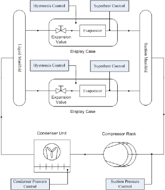
Figure 1: Layout of a simple supermarket refrigeration system.

In a typical supermarket refrigeration system, the temperature in each display case is controlled by a hysteresis controller that opens the expansion valve when the air temperature $T$ (measured near to the foodstuffs) reaches a predefined upper temperature limit $T^{u}$. The valve stays open until $T$ decreases to the lower temperature limit $T^{l}$. At this point, the controller closes the valve again. Practice reveals that if the display cases are similar, the hysteresis controllers have tendency to synchronize the display cases [7]. It means that the air temperatures $T_{i}$ for $i\in\{1,\ldots,N\}$, where $N$ is the number of display cases, tend to match as time progresses.

In the sequel we discuss, for simplicity, a model of a refrigeration system that consists of only two identical display cases and a compressor. The dynamics of the air temperature $T_{i}$ for display case $i\in\{1,2\}$ and the suction pressure $P$ for the system of two display cases are governed by the following system of equations,

$$\dot{x}=\xi_{\delta}(x)=A_{\delta}x+B_{\delta},$$ (1)

where

$$A_{\delta}=\begin{bmatrix}-a-\delta_{1}c&0&\delta_{1}d\\ 0&-a-\delta_{2}c&\delta_{2}d\\ 0&0&-\alpha\end{bmatrix},~{}B_{\delta}=\begin{bmatrix}b+e\delta_{1}\\ b+e\delta_{2}\\ \beta+\delta_{1}+\delta_{2}\end{bmatrix},~{}x=\begin{bmatrix}T_{1}\\ T_{2}\\ P\end{bmatrix},$$

with $a,b,c,d,e,\alpha,\beta$ constants whose specific values are provided in Appendix 6.1, and $\delta=(\delta_{1},\delta_{2})\in\mathbf{2}^{2}$ with $\mathbf{2}=\{0,1\}$ and $\delta_{i}\in\{0,1\}$ the switching parameter for display case $i$; it indicates whether the expansion valve is closed ($\delta_{i}=0$) or open ($\delta_{i}=1$). The switching law is given by the hysteresis control:

$${\delta_{i}=\begin{cases}1&\text{if}~{}T_{i}\geq T_{i}^{u}\\ 0&\text{if}~{}T_{i}\leq T_{i}^{l}\\ \delta_{i}&\text{if}~{}T_{i}^{l}<T_{i}<T_{i}^{u},\end{cases}}$$ (2)

where $T_{i}^{u}$ and $T_{i}^{l}$ are respectively the predefined upper and lower temperature limits for display case $i$. By convention, $\delta_{i}=0$ for any initial condition $T_{i}(t_{0})=T_{i}^{0}\in]T_{i}^{l},T_{i}^{u}[$. Such an initial condition is assumed throughout this paper; hence, (2) is well defined.

3 Refrgeration system as a hybrid system

Consider the following scenario. Let $x(t_{0})~{}\in~{}]T_{1}^{l},T_{1}^{u}[\times]T_{2}^{l},T_{2}^{u}[\times\mathbb{R}_{+}$, and $\delta=(0,0)$; thereby, both display cases are initially switched off. Suppose that at time $t$, the air temperature $T_{i}$ of the $i$th display case reaches the upper temperature limit $T_{i}^{u}$, then the $i$th display case is switched on, and $\delta_{i}=1$. This scenario indicates that the refrigeration system (1) comprises four dynamical systems, each defined on a copy of the polyhedral set

$$Q=[T_{1}^{l},T_{1}^{u}]\times[T_{2}^{l},T_{2}^{u}]\times\mathbb{R}_{+},$$ (3)

as illustrated in Fig. 2.

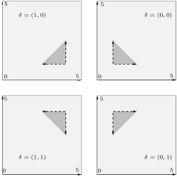
Figure 2: The state space of the refrigeration system consisting of two display cases is illustrated. Here, the pressure axis is suppressed, and $(T^{l}_{i},T^{u}_{i})=(0,5)$. The direction of the vector field $\xi_{\delta}$ is indicated by the dark shaded triangles (see Proposition 1 in [13]).

A discrete transition between these four systems takes place whenever a trajectory reaches one of the following four facets of $Q$

$$F^{\alpha}_{1} =F^{\alpha}_{1}(Q)=\delta^{\alpha}[T_{1}^{l},T_{1}^{u}]\times[T_{2}^{l},T_{2}^{u}]\times\mathbb{R}_{+}~{}\hbox{ and }~{}$$

$$F^{\alpha}_{2} =F^{\alpha}_{2}(Q)=[T_{1}^{l},T_{1}^{u}]\times\delta^{\alpha}[T_{2}^{l},T_{2}^{u}]\times\mathbb{R}_{+},$$

with $\alpha\in\mathbf{2}$ and $\delta^{0}[a,b]=\{a\}$, $\delta^{1}[a,b]=\{b\}$.

Moreover, the transitions between subsystems can be describe by eight reset maps $R_{i}(\delta):F_{i}^{l_{i}(i,\delta)}\times\{\delta\}\to F_{i}^{l_{i}(i,\delta)}\times\{l(i,\delta)\}$ defined by $R_{i}(\delta)\left(x,\delta\right)=(x,l(i,\delta))$ with

$$l(i,\delta)=(l_{1}(i,\delta),l_{2}(i,\delta))=\left\{\begin{matrix}(\delta_{1}+1,\delta_{2})&\hbox{if}&i=1\\ (\delta_{1},\delta_{2}+1)&\hbox{if}&i=2,\end{matrix}\right.$$

where the results of the summation are computed modulo $2$. Intuitively, the map $l$ takes a polyhedral set enumerated by $\delta$ to the future polyhedral set. The variable $i$ indicates that the discrete transition takes place when the temperature $T_{i}$ reaches its upper or lower boundary. The domain of a reset map, will be referred to as a switching surface. Specifically, a switching surface is a facet of one of the polyhedral sets making up the state space of the refrigeration system (1).

The above construction allows us to identify the refrigeration system as a switched hybrid system. More precisely, let ${\cal P}=\{P_{\delta}~{}|~{}P_{\delta}=Q\times\{\delta\},~{}\delta\in{\mathbf{2}}^{2}\}$ consist of the four polyhedral sets making up the state space, ${\cal S}=\{\xi_{\delta}~{}|~{}\xi_{\delta}(x)=A_{\delta}x+B_{\delta},~{}\delta\in{\mathbf{2}}^{2}\}$ consist of the four dynamical systems, and $\mathcal{R}=\{R_{i}(\delta)~{}|~{}(i,\delta)\in\{1,2\}\times\mathbf{2}^{2}\}$ consist of the eight reset maps. Then the triple $({\cal P},{\cal S},{\cal R})$ constitute a hybrid system as defined in Appendix 6.2. Hence the behavior of the system is expressed by means of a (hybrid) trajectory which heuristically can be described simply as the union of trajectories generated by four local dynamical systems, see Appendix 6.3 for a precise describtion.

With this notion at hand we say that a refrigeration system exhibit asymptotic synchronization if there exists a $(T,l)$-periodic trajectory which is asymptotically stable in $X^{*}$ [6, Definition 13.3], where $X^{*}$ denote the quotient space $X/\sim$ with $X=\bigcup_{\delta\in{\mathbf{2}}^{2}}P_{\delta}$ and $\sim\subset X\times X$ the equivalence relation, [3], generated by the reset maps in $\mathcal{R}$. For a detailed explanation see [13], where it is also shown that the refrigeration system generates an asymptotically stable $(T_{p},2)$-periodic trajectory, with $T_{p}\approx 261$, lying on the diagonal of $P_{(0,0)}$ and $P_{(1,1)}$.

The (hybrid) refrigeration system with two display cases is illustrated in Fig. 3. Here, each element of $\cal P$ has been (orthogonally) projected onto the $(T_{1},T_{2})$-space. Hence, the polyhedral sets $P_{\delta}$ are represented by cubes. The three cubes $P_{(0,1)}$, $P_{(1,0)}$, $P_{(1,1)}$ have been vertically and/or horizontally reflected (compare with Fig. 2). The stippled lines in the drawing indicate the reset maps in $\cal R$.

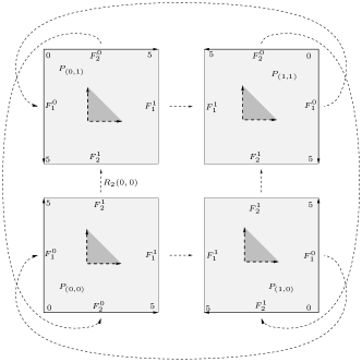
Figure 3: The $T_{1}T_{2}$-state space of the refrigeration system consists of two display cases. The reset maps are indicated by the stippled lines (see Fig. 2 and its caption for further explanation). The pressure axis has been suppressed; thus, each $P_{\delta}=Q\times\{\delta\}$ is illustrated by a square. By abuse of notation, the facets of $P_{\delta}$ are denoted by $F_{i}^{\alpha}$ (instead of $F_{i}^{\alpha}\times\{\delta\}$).

4 Stochastic analysis of synchronisation

So far, the discrete transition from a local system to another has been described as deterministic. In other words, it take place with probability one when a trajectory “hits” a switching surface. However, from a practical point of view, this causes a problem. For instance, any sampling step will result in the trajectory “hitting” the switching surface with probability zero. On account of model uncertainty, noise, and most of all the inaccuracy of temperature measurement, the switching surface should therefore be “thickened” by replacing each switching surface with an open neighborhood of it.

In the sequel, we incorporate the “thickening of switching surfaces” into our model of the refrigeration system. Specifically, we construct an open neighborhood around the switching surfaces within which a probability measure on each trajectory is proposed. Afterwards, we use this measure to describe the probability of a discrete transition, in such a way that the longer a trajectory stays within the neighborhood the higher becomes the probability of a transition. This makes it possible to devise a method for analyzing the typical behavior of the system, as well as a way of visualizing it.

Let $U$ be a stochastic variable uniformly distributed on $[-\epsilon,\epsilon]$ with density function $p(u)=\mathbf{I}_{[-\epsilon,\epsilon]}(u)/2\epsilon$, where $\mathbf{I}_{A}$ denotes the indicator function of a set $A$. Consequently, the distribution of $U$ can be described by the survivor function

$$S(u)=1-\int_{-\epsilon}^{u}p(v)dv=\begin{cases}1&u<-\epsilon\\ 1-(u+\epsilon)/2\epsilon&|u|\leq\epsilon\\ 0&u>\epsilon,\end{cases}$$

which is the probability of $U\geq u$, $\textbf{P}(U\geq u)$. The distribution of $U$ can also be described by its conditional intensity (or hazard) function $h(u)=p(u)/S(u)=\mathbf{I}_{[-\epsilon,\epsilon]}(u)/(\epsilon-u)$. Heuristically, a small variation of $h(u)$ is the probability of $U$ being in a small region around $u$ conditional on $U$ not being smaller than $u$, $\textbf{P}(U\in du~{}|~{}U\geq u)$. The conditional intensity function, for short intensity, turns out to be a convenient starting point for defining stochastic transitions between the different local dynamical systems.

To this end, we derive an intensity function suitable for our purpose. Recall the notation introduced in Section 6.2, and let $F(\delta)=F_{1}^{l_{1}(1,\delta)}\cup F_{2}^{l_{2}(2,\delta)}$ denote the union of switching surfaces in the polyhedral set $P_{\delta}$. Furthermore, let $F(\delta)^{\epsilon}$ denote the $\epsilon$-neighborhood of $F(\delta)$ in $\mathbb{R}^{3}$.

For $x\in F(\delta)^{\epsilon}$, let $F_{i}^{l_{i}(i,\delta)}$ be a switching surface within $\epsilon$ (Hausdorff) distance to $x$, and define $x_{(i,\delta)}=x-\pi_{(i,\delta)}(x)$, where $\pi_{(i,\delta)}$ is the orthogonal projection onto $F_{i}^{l_{i}(i,\delta)}$. Hence, when $x_{(i,\delta)}$ is non-zero, it is a normal vector to $F_{i}^{l_{i}(i,\delta)}$ (more precisely, to the affine hull of $F_{i}^{l_{i}(i,\delta)}$). It points into $P_{\delta}$ when $x\in P_{\delta}-F_{i}^{l_{i}(i,\delta)}$ and out of $P_{\delta}$ when $x\in F(\delta)^{\epsilon}-P_{\delta}$. Let $n_{(i,\delta)}$ denote a normal vector to $F_{i}^{l_{i}(i,\delta)}$ which points out of $P_{\delta}$. By means of the above quantities, we define the parameter $u_{(i,\delta)}(x)=|x_{(i,\delta)}|\text{sign}\langle n_{(i,\delta)},x_{(i,\delta)}\rangle$ where $x_{(i,\delta)}=x_{(i,\delta)}(x)$ is regarded as a function of $x$.

Now let $\gamma(t;k)$ denote a trajectory (see Appendix 6.3) of the refrigeration system, and assume that $\gamma(t;k)$ follows system $\delta$, i.e., $\dot{\gamma}(t;k)=\xi_{\delta}(\gamma(t;k))$. The intensity function $h_{(i,\delta)}$ for switching from system $\delta$ to system $l(i,\delta)$ at $\gamma(t;k)$ can now be defined as

$$h_{(i,\delta)}(\gamma(t;k))=\begin{cases}0&u_{ij}(\gamma(t;k))<-\epsilon\\ h(u_{ij}(\gamma(t;k)))&|u_{ij}(\gamma(t;k))|\leq\epsilon\\ \infty&u_{ij}(\gamma(t;k))>\epsilon.\end{cases}$$

Hence, $h_{(i,\delta)}(\gamma(t;k))$ is the intensity of the signed orthogonal distance from $\gamma(t;k)$ to the switching surface $F_{i}^{l_{i}(i,\delta)}$ in the $\epsilon$-neighborhood of $P_{\delta}$. As a result, any trajectory whose intersection with the $\epsilon$-neighborhood of $F_{i}^{l_{i}(i,\delta)}$ is contained in a normal subspace to $F_{i}^{l_{i}(i,\delta)}$ will switch according to the uniform distribution on the restriction of the trajectory to the $\epsilon$-neighborhood.

The above construction successfully copes with switching for which a trajectory reaches one switching region at a time. To deal with the situation where a point of switching is within distance $\epsilon$ to both switching surfaces, we will assume that switching to each of the systems will happen independently. With this assumption, we immediately conclude that if $\gamma(t;k)$ follows system $\delta$, and is within distance $\epsilon$ from both $F_{2}^{l_{2}(2,\delta)}$ and $F_{2}^{l_{2}(2,\delta)}$ then the intensity function $h_{\delta}$ for switching from system $\delta$ to system $l(i,\delta)$ at $\gamma(t;k)$ is given by $h_{\delta}(\gamma(t;k)(t))=h_{(1,\delta)}(\gamma(t;k))+h_{(2,\delta)}(\gamma(t;k))$. Thus, if the discrete transition occurs at $\gamma(t;k)$, the switch to the system $l(i,\delta)$ happens with probability $h_{(i,\delta)}(\gamma(t;k))/h_{(\delta)}(\gamma(t;k)).$ Equivalently, we can allow switching to happen according to all of the intensities $h_{(1,\delta)}(\gamma(t;k))$ and $h_{(2,\delta)}(\gamma(t;k))$ independently of each other and disregard all the switchings except the first one which determines the switching.

Based on the above theory and numerical simulations, we now conduct synchronization analysis of the refrigeration system when switching noise is present. To begin with, we describe how the theory is implemented in simulation. For this, we follow Algorithm 7.4III in [4, p. 260].

When a trajectory enters the switching region $F(\delta)^{\epsilon}$, an exponentially distributed variable with mean one is simulated. Thereafter, for each sample, the intensity is calculated, and subsequently the integral of the intensity is computed inductively. Afterwards, the exponentially distributed variable is compared with the number obtained by the integral computation [4, p. 258 (Lemma 7.4II)]. As a consequence, the switching occurs at the sample point where the integral exceed the exponentially distributed variable.

In the above setup, the system trajectories become stochastic; hence, we can apply concepts such as mean values to describe the system behavior. For a trajectory $(\gamma,\mathcal{T}_{\infty})$, $A\subset X$ and $I=[t^{\prime},t^{\prime\prime}]\subset[0,\infty)$, let $Z_{\gamma}(A,I)$ be the arc length from $t^{\prime}$ to $t^{\prime\prime}$ of $\gamma$ inside $A$. As a consequence, $\gamma\mapsto Z_{\gamma}(A,I)$ defines a non-negative random variable, whose mean $\mathbb{E}[Z(A,I)]$ describes the curve intensity relative to $(A,I)$. The curve intensity measures the typical behavior of trajectories by the mean length of trajectories on $I$ inside $A$.

We illustrate the typical behavior of the refrigeration system with two display cases by simulation of the curve intensity. For this purpose, we use the following algorithm: (1) Fix a time interval $I\subset[0,\infty)$ and a sufficiently regular subset $A\subset X$. (2) Simulate $n$ trajectories $\gamma_{1},\dots\gamma_{n}$. (3) Divide $A$ into small subsets $A_{i}$. (4) Calculate $\mathbb{E}[Z(A_{i},I)]\approx\frac{1}{n}\sum_{j}Z_{\gamma_{j}}(A_{i},I)$ where $Z_{\gamma_{j}}(A_{i},I)$ is approximated by the number of sampling points (on trajectories) falling in $A_{i}$.

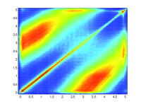
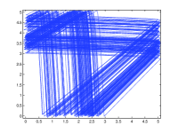
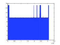
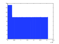
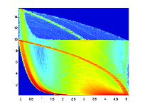
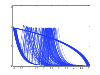
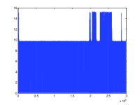
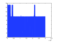
Figure 4: Each of the plots in column one and two are illustrated on various projections of the space obtained by identifying the four copies of $Q$ in (3) used to define the state space of the refrigeration system. The first column represents intensity plots, $\epsilon=0.1,~{}I=[0,10^{6}]$, based on $n=10$ trajectories at the point $(0,0,15.23)$ on the asymptotically stable $(T_{p},2)$-periodic trajectory found in [13] (top: $T_{1}T_{2}$-plane, bottom: $T_{1}P$-plane). The second column represents one of the ten trajectories in a subinterval of $I$ (top: $T_{1}T_{2}$-plane, bottom: $T_{1}P$-plane) shown in the time interval $[10^{6},1.1\cdot 10^{6}]$. The last two columns represent four of the ten simulations and show the sample-time evolution of suction pressure $P$.

Intensity plots for $I=[0,10^{6}]$, $\epsilon=0.1$ and $n=10$ have been generated for initial values both within and outside the basin of attraction of the asymptotically stable $(T_{p},2)$-periodic trajectory found in [13]. The resulting intensity plots are similar to the one illustrated in the first column of Figure 4. Contrarily to the deterministic behavior, the system synchronizes occasionally over the time interval $I$, as seen in the last two columns of Figure 4, where the pressure peaks at $15.23$ correspond to the presence of the $(T_{p},2)$-periodic trajectory (synchronization). The behavior of the system in the remaining time is indicated in the first column of Figure 4 as the colored area except for the diagonal (top) and yellow/green circle through $(0,15.23)$, and in the last two columns as pressure peaks at $10$. We remark that the peaks at $10$ do not correspond to another limit cycle, as shown in the second column of Figure 4 (in fact this correspond to the interval $[10^{6},1.1~{}10^{6}]$ of the plot in the right lower corner).

Further simulations reveal that the time spent in the $(T_{p},2)$-periodic trajectory is highly dependent on $\epsilon$. For $\epsilon=0.1$, relatively little time is spent in the $(T_{p},2)$-periodic trajectory, whereas for $\epsilon=0.01$, the behavior closely matches that of the deterministic case. More precisely, for $\epsilon=0.01$ and initial values in the basin of attraction, the system rapidly converges to the $(T_{p},2)$-periodic trajectory and stays close to it with a high probability, while for initial values outside the basin of attraction, the system has a small probability of converging to the $(T_{p},2)$-periodic trajectory within the time interval $I$. As a consequence, the relative frequency of appearance of the $(T_{p},2)$- trajectory can be described as a monotonically decreasing function $f(\epsilon)\in[0,1]$, where $f(0)=1$ corresponds to the deterministic case.

In summary, uncertainties of the temperature measurements influence synchronization and can be used to design de-synchronization scheme. We conclude that adding noise as above to temperature measurements de-synchronizes the refrigeration system: An increase in measurement uncertainty yields a decrease of the prevalence of synchronization.

5 Conclusion

In this paper, we have investigate the influence of switching noise on the synchronization phenomenon in supermarket refrigeration systems. We have developed a numerical method for computing intensity plots. By analyzing them, we have concluded that the time the refrigeration system stays synchronized is dependent on uncertainties of the temperature measurements. A greater measurement uncertainty yields a smaller accumulated time in which the refrigeration system is in synchronization.

6 Appendix

6.1 Model of refrigeration system

The mathematical model presented here is a summary of the model developed in [12]. For the $i$th display case, dynamics of the air temperature $T_{air,i}$ can be formulated as

$$\frac{{d}T_{air,i}}{{d}t}=\frac{\dot{Q}_{goods-air,i}+\dot{Q}_{load,i}-\delta_{i}\dot{Q}_{e,max,i}}{\left(1+\frac{UA_{goods-air,i}}{UA_{air-wall,i}}\right)M_{wall,i}C_{p,wall,i}}~{}~{}\hbox{ with }$$ (4a)

$$T_{wall,i}=T_{air,i}-\frac{\dot{Q}_{goods-air,i}+\dot{Q}_{load,i}}{UA_{air-wall,i}},$$ (4b)

$$\dot{Q}_{goods-air,i}=UA_{goods-air,i}(T_{g0,i}-T_{air,i}),$$ (4c)

$$\dot{Q}_{e,max,i}=UA_{wall-ref,max,i}(T_{wall,i}-a_{T}P_{suc}-b_{T}),$$ (4d)

where the process parameters are specified in Table 1, and $\delta_{i}\in\{0,1\}$ is the switch parameter for the $i$th display case. When $\delta_{i}=0$, the $i$th expansion valve is switched off, whereas when $\delta_{i}=1$ it is switched on. The suction manifold dynamics is governed by the differential equation

$$\frac{{d}P_{suc}}{{d}t}=\frac{\textstyle\sum_{i=1}^{k}\delta_{i}\dot{m}_{0,i}+\dot{m}_{r,const}-\dot{V}_{comp}(a_{\rho}P_{suc}+b_{\rho})}{V_{suc}\cdot\nabla\rho_{suc0}},$$ (5)

where $N$ is the number of display cases, and $\dot{m}_{0,i}=\dot{m}_{0}$ for $i\in\{1,\ldots,N\}$.

We denote $T_{i}=T_{air,i}$ and $P=P_{suc}$ and write the dynamics of the air temperature and suction pressure in the concise form (with the process constants in (4a) collected in $a,b,c,d,e,\alpha,\beta$ and then replaced by their numerical values)

$$\dot{T}_{i} =-aT_{i}+b-\delta_{i}(cT_{i}-dP-e)$$ (6a)

$$=-0.0019T_{i}+0.0244-\delta_{i}(-0.0012T_{i}+0.0506P+0.1065),$$

$$\dot{P} =-\alpha P+\beta+\delta_{1}+\delta_{2}=-0.056P+0.0038+\delta_{1}+\delta_{2}.$$ (6b)

Display cases
$UA_{wall-ref,max}$	500 $\frac{J}{s\cdot K}$	$T_{g0}$	3.0 ${}^{0}C$
$UA_{goods-air}$	300 $\frac{J}{s\cdot K}$	$\dot{m}_{0}$	1.0 $kg/s$
$UA_{air-wall}$	500 $\frac{J}{s\cdot K}$	$\dot{Q}_{load}$	3000 $J/s$
$\dot{m}_{r,const}$	0.2 $\frac{kg}{s}$	$M_{wall}$	260 $kg$
$\nabla\rho_{suc0}$	4.6 $\frac{kg}{m^{3}bar}$	$C_{p,wall}$	385 $\frac{J}{kg\cdot K}$
The same parameters has been used for all display cases.
Compressor
$\dot{V}_{comp}$	0.28 $\frac{m^{3}}{s}$
Suction manifold
$V_{suc}$	5.00 $m^{3}$
Air temperature control
$T_{i}^{l}$	0.00 ${}^{0}C$	$T_{i}^{u}$	5.00 ${}^{0}C$
Coefficients
$a_{T}=-16.2072$	$b_{T}={-41.9095}$	$a_{\rho}=4.6$	$b_{\rho}=0.4$

Table 1: Parameters for a simplified supermarket refrigeration system

6.2 Hybrid systems

A detailed study of the hybrid system presented below can be found in [9]. We write $F\prec P$ if $F$ is a face of the polyhedral set $P$. A map $f:P\to P^{\prime}$ is polyhedral if 1) it is a continuous injection, and 2) for any $F\prec P$ there is $F^{\prime}\prec P^{\prime}$ with $\dim(F)=\dim(F^{\prime})$ such that $f(F)\subseteq F^{\prime}$.

Definition 1 (Hybrid System)

For finite index sets $J$ and $D$, a hybrid system (of dimension $n$) is a triple $({\cal P},{\cal S},{\cal R})=({\cal P}_{D},{\cal S},{\cal R}_{J})$, where

1. $\mathcal{P}=\{P_{\delta}\subset\mathbb{R}^{n}~{}|~{}P_{\delta}\hbox{ a polyhedral set},\dim(P_{\delta})=n,~{}\delta\in D\}$ is a family of polyhedral sets.

2. ${\cal S}=\{\xi_{\delta}:P_{\delta}\rightarrow\mathbb{R}^{n}~{}|~{}P_{\delta}\in{\cal P},~{}{\delta}\in D\}$ is a family of smooth vector fields.

3. ${\cal R}=\{R_{j}:F\rightarrow F^{\prime}~{}|~{}F\prec P\in{\cal P},~{}F^{\prime}\prec P^{\prime}\in{\cal P},~{}\dim(F)=\dim(F^{\prime})=n-1,~{}j\in J\}$ is a family of polyhedral maps, called reset maps.

After identifying $D$ with a finite subset of $\mathbb{R}$, we can rewrite the hybrid system $({\cal P}_{D},{\cal S},{\cal R}_{J})$ as Fig.

$$\frac{\mathrm{d}}{\mathrm{d}t}(x,q) \in \bar{F}(x,q)=\{(\xi_{q}(x),0)|~{}x\in P_{q}\}~{}\hbox{ for }(x,q)\in\bar{C},\hbox{ and }$$

$$(x,q)^{+}\in\{R_{k}(x,q)|~{}x \in \bar{G}(x,q)=\mathrm{dom}(R_{k})\prec P_{q}\}~{}\hbox{ for }(x,q)\in\bar{D},$$

where $\bar{C}=\bigcup_{\delta\in D}(P_{\delta}\times\{\delta\})$ and $\bar{D}=\bigcup_{\{(\delta,j)\in D\times J~{}|~{}\mathrm{dom}(R_{j})\prec P_{\delta}\}}(\mathrm{dom}(R_{j})\times\{\delta\})$. This is precisely the hybrid system in [5].

6.3 Trajectories of a refrigeration system

We bring in a concept of a (hybrid) time domain [5]. Let $k\in\mathbb{N}\cup\{\infty\}$; a subset $\mathcal{T}_{k}\subset\mathbb{R}_{+}\times\mathbb{Z}_{+}$ will be called a time domain if there exists an increasing sequence $\{t_{i}\}_{i\in\{0,\ldots,k\}}$ in $\mathbb{R}_{+}\cup\{\infty\}$ such that

$$\mathcal{T}_{k}=\bigcup_{i\in\{1,\ldots,k\}}T_{i}\times\{i\}$$

where $T_{i}=[t_{i-1},t_{i}]\hbox{ if }i\in\{1,\dots,k-1\},\hbox{ and }T_{k}=\left\{\begin{matrix}[t_{k-1},t_{k}]\hbox{ if }t_{k}<\infty\\ [t_{k-1},\infty[\hbox{ if }t_{k}=\infty.\end{matrix}\right.$

Note that $T_{i}=[t_{i-1},t_{i}]$ for all $i$ if $k=\infty$. We say that the time domain is infinite if $k=\infty$ or $t_{k}=\infty$. The sequence $\{t_{i}\}_{i\in\{0,\ldots,k\}}$ corresponding to a time domain will be called a switching sequence.

Definition 2 (Trajectory)

A trajectory of the hybrid system $({\cal P}_{D},{\cal S},{\cal R}_{J})$ is a pair $({\cal T}_{k},\gamma)$ where $k\in\mathbb{N}\cup\{\infty\}$ is fixed, and

• $\mathcal{T}_{k}\subset\mathbb{R}_{+}\times\mathbb{Z}_{+}$ is a time domain with corresponding switching sequence $\{t_{i}\}_{i\in\{0,\ldots,k\}}$,

• $\gamma:\mathcal{T}_{k}\to X=\bigcup_{\delta\in D}P_{\delta}\times\{\delta\}$ is continuous ($X$ has the disjoint union topology) and satisfies:

  1. For each $i\in\{1,\ldots,k-1\}$, there exist $\delta\neq\delta^{\prime}\in D$ such that $\gamma(t_{i};i)\in\text{bd}(P_{\delta})$, and $\gamma(t_{i};i+1)\in\text{bd}(P_{\delta^{\prime}})$.

  2. For each $i\in\{1,\ldots,k\}$, there exists $\delta\in D$ such that the Cauchy problem $\frac{\partial}{\partial t}\gamma(t;i)=\dot{\gamma}(t;i)=\xi_{\delta}(\gamma(t;i)),~{}\gamma(t_{i-1};i)=x_{i-1}\in P_{\delta},$ has a solution on $T_{i}\subset\mathcal{T}_{k}$.

  3. For each $i\in\{1,\ldots,k-1\}$, there exists $j\in J$ such that $R_{j}(\gamma(t_{i};i))=\gamma(t_{i};i+1)$.

A trajectory at $x$ is a trajectory $({\cal T}_{k},\gamma)$ with $\gamma(t_{0};1)=x$. By abuse of notation $\gamma$ will sometimes be referred to as a trajectory.

The next definition formalizes the notion of a periodic trajectory, which will be used in defining synchronization of the refrigeration system.

Definition 3 ($(T,l)$-periodic trajectory)

Let $(T,l)\in\mathbb{R}_{+}\times\mathbb{Z}_{+}$. A trajectory $({\cal T}_{k},\gamma)$ is $(T,l)$-periodic (or just periodic) if (1) ${\cal T}_{k}$ is an infinite time domain, and (2) for any $i\in\{1,\ldots,k\}$ and $t\in p({\cal T}_{k})$, where $p:{\cal T}_{k}\to[t_{0},\infty[$ is the projection $p(t,i)=t$, we have $\gamma(t+T;i+l)=\gamma(t;i)$.

In particular, if $({\cal T}_{k},\gamma)$ is a $(T,l)$-periodic trajectory, and $T$ is nonzero then $p:{\cal T}_{k}\to[t_{0},\infty[$ is surjective.

References

- [1]
- [2] I. I. Blekhman, A. L. Fradkov, H. Nijmeijer & A. Yu. Pogromsky (1997): On self-synchronization and controlled synchronization. Systems Control Lett. 31(5), pp. 299–305, 10.1016/S0167-6911(97)00047-9.
- [3] G. E. Bredon (1997): Topology and geometry. Graduate Texts in Mathematics 139, Springer-Verlag, New York, 10.1007/978-1-4757-6848-0.
- [4] D. J. Daley & D. Vere-Jones (2003): An introduction to the theory of point processes. Vol. I, second edition. Probability and its Applications (New York), Springer-Verlag, New York, 10.1007/978-0-387-49835-5.
- [5] R. Goebel, R. G. Sanfelice & A. R. Teel (2009): Hybrid dynamical systems: robust stability and control for systems that combine continuous-time and discrete-time dynamics. IEEE Control Syst. Mag. 29(2), pp. 28–93, 10.1109/MCS.2008.931718.
- [6] W. M. Haddad, V. Chellaboina & S. G. Nersesov (2006): Impulsive and hybrid dynamical systems. Princeton Series in Applied Mathematics, Princeton University Press, Princeton, NJ, 10.1515/9781400865246.
- [7] L.F.S. Larsen, C. Thybo, R. Wisniewski & R. Izadi-Zamanabadi (2007): Synchronization and desynchronizing control schemes for supermarket refrigeration systems. In: 16th IEEE International Conference on Control Applications. Part of IEEE Multi-conference on Systems and Control, IEEE, pp. 1414–1419, 10.1109/CCA.2007.4389434.
- [8] J. Leth, J. G. Rasmussen, H. Schioler & R. Wisniewski (2012): A class of stochastic hybrid systems with state-dependent switching noise. In: Decision and Control (CDC), 2012 IEEE 51st Annual Conference on, pp. 4737–4744, 10.1109/CDC.2012.6427010.
- [9] J. Leth & R Wisniewski (2014): Local analysis of hybrid systems on polyhedral sets with state-dependent switching. Applied Mathematics and Computer Science 24(2), pp. 341–355, 10.2478/amcs-2014-0026.
- [10] A. Pikovsky & Y. Maistrenko, editors (2003): Synchronization: theory and application. NATO Science Series II: Mathematics, Physics and Chemistry 109, Kluwer Academic Publishers, Dordrecht, 10.1007/978-94-010-0217-2.
- [11] C. Thybo & L. F. S. Larsen (2011): Methods of Analysing a Refrigeration Sytem and a Method of Controlling a Refrigeration Systems. US patent 2011/0289948 A1.
- [12] R. Wisniewski & L. F. S. Larsen (2008): Method for analysis of synchronization applied to supermarket refrigeration system. In: 17th IFAC World Congress, 17, 10.3182/20080706-5-KR-1001.3621.
- [13] R. Wisniewski & J. Leth (2014): Analysis of Synchronization in a Supermarket Refrigeration System. Control Theory and Technology 12(2), pp. 154–162, 10.1007/s11768-014-0077-2.