The Role of Turbulence and Magnetic Fields in Simulated Filamentary Structure

Helen Kirk^*^*affiliation: Banting Fellow ¹¹affiliation: Origins Institute, McMaster University, Hamilton, ON, L8S 4M1, Canada ²²affiliation: Department of Physics and Astronomy, McMaster University, Hamilton, ON, L8S 4M1, Canada ³³affiliation: National Research Council Canada, Herzberg Astronomy and Astrophysics, Victoria, BC, V9E 2E7, Canada; helen.kirk@nrc-cnrc.gc.ca , Mikhail Klassen²²affiliation: Department of Physics and Astronomy, McMaster University, Hamilton, ON, L8S 4M1, Canada , Ralph Pudritz¹¹affiliation: Origins Institute, McMaster University, Hamilton, ON, L8S 4M1, Canada ²²affiliation: Department of Physics and Astronomy, McMaster University, Hamilton, ON, L8S 4M1, Canada , Samantha Pillsworth²²affiliation: Department of Physics and Astronomy, McMaster University, Hamilton, ON, L8S 4M1, Canada ⁴⁴affiliation: Saint Mary’s University, Department of Astronomy and Physics, Halifax, NS, B3H 3C3, Canada

Abstract

We use numerical simulations of turbulent cluster-forming regions to study the nature of dense filamentary structures in star formation. Using four hydrodynamic and magnetohydrodynamic simulations chosen to match observations, we identify filaments in the resulting column density maps and analyze their properties. We calculate the radial column density profiles of the filaments every 0.05 Myr and fit the profiles with the modified isothermal and pressure confined isothermal cylinder models, finding reasonable fits for either model. The filaments formed in the simulations have similar radial column density profiles to those observed. Magnetic fields provide additional pressure support to the filaments, making ‘puffier’ filaments less prone to fragmentation than in the pure hydrodynamic case, which continue to condense at a slower rate. In the higher density simulations, the filaments grow faster through the increased importance of gravity. Not all of the filaments identified in the simulations will evolve to form stars: some expand and disperse. Given these different filament evolutionary paths, the trends in bulk filament width as a function of time, magnetic field strength, or density, are weak, and all cases are reasonably consistent with the finding of a constant filament width in different star-forming regions. In the simulations, the mean FWHM lies between 0.06 and 0.26 pc for all times and initial conditions, with most lying between 0.1 to 0.15 pc; the range in FWHMs are, however, larger than seen in typical Herschel analyses. Finally, the filaments display a wealth of substructure similar to the recent discovery of filament bundles in Taurus.

1. Introduction

Filaments appear to be an important ingredient in the formation of stars. While filaments have been known to be associated with star forming regions for decades (e.g., Schneider79; Bally87), observations from the Herschel Space Telescope, particularly the Gould Belt (Andre10) and HOBYS (Motte10) Legacy Surveys have underlined the prevalence of filamentary structures within star forming regions. With Herschel’s unprecedented ability to sensitively map large areas of the sky, several common properties of filaments have now been identified. First, filaments appear to not be well represented by the Ostriker64 equilibrium model of an isothermal cylinder; the column density profile is shallower (e.g., Arzoumanian11). This may indicate that magnetic fields (e.g., FiegePudritz00a) contribute to supporting the filament from collapse, although Smith14 demonstrate that filaments formed in purely turbulent environments also have a similarly shallow slope. Rotation may also lead to a shallower slope (Recchi14). Second, the mass per unit length of filaments appears to correlate with star-formation activity: filaments with mass per unit length less than the value needed for collapse of an isothermal cylinder (Ostriker64) tend to be associated with regions which are forming few if any stars, while filaments with supercritical mass per unit length values tend to be associated with active star forming regions (e.g., Arzoumanian11; Hennemann12). What is still unclear, however, is what forces dominate the formation and evolution of the filaments, and how the filaments contribute to star formation. For example, are the filaments formed primarily through turbulent shocks, or under the influence of magnetic fields or gravity? Does turbulence control the ability of filaments to fragment into star-forming cores? What forces set the observed (column) density profiles? And do filaments primarily provide a denser collection of gas to promote local star formation (e.g. Hacar11), or do they play a significant role in providing a conduit of mass for the formation of larger stellar clusters, which appear to form preferentially at the intersection of several filaments (see e.g., Myers09; Myers11; Schneider12; Hennemann12; Kirk13)?

In this paper, we investigate the first of these issues, namely the formation and evolution of filaments, through the analysis of our numerical simulations. We compare the column density properties of filaments formed within four different simulations: higher and lower density, and with and without magnetic fields. These analyses provide a complementary look at simulations to those recently published in Smith14, where the influence of different types of turbulence on filament properties was examined, but the effect of the inclusion of magnetic fields or differing initial mean densities was not.

We find that while the largest-scale structures in the gas are set by turbulent motions, and appear similar in all four simulations, magnetic fields and gravity do influence the properties of individual filaments. In particular, magnetic fields cushion the initial turbulent gas compressions, leading to filaments which are initially less condensed, and subsequently evolve more slowly (due to the weaker gravitational pull) than the corresponding hydrodynamic case. We note that the simulations we analyze were only able to be run for a few tenths of the global free-fall time, limiting our sensitivity to later-time evolutionary trends. The simulated filaments have properties which are consistent with those measured in real filaments characterized by Herschel, suggesting that the general insights gained with these simulations are applicable to real molecular clouds. Finally, turbulence and magnetic fields, and not just the thermal properties of molecular gas, appears to set the critical conditions for gravitational instability leading to star formation.

In what follows, we first discuss our numerical methods and simulations (Section 2), discuss the basic filament properties resulting from the simulations (Section 3), compare various models of filament structure (Section 4), and examine the effects of spatial resolution in characterizing filaments (Section 5). We discuss our results and their implications, as well as the limitations of our present analysis in Section 6.

2. Numerical Methods

2.1. Simulation Setup

We used the flash hydrodynamics code (Fryxell2000) version 2.5 to perform numerical simulations of molecular clumps, i.e., parsec-scale condensations of gas capable of forming a cluster of stars. flash solves the fluid-dynamical equations on an adaptive Eulerian grid, making use of the paramesh library (Olson+1999; MacNeice+2000). It includes self-gravity, Lagrangian sink particles to represent gravitationally collapsing cores and (proto)stars (Banerjee2009; Federrath2010), and gas cooling by dust and by molecular lines (Banerjee+2006). Stellar properties are self-consistently evolved via a one-zone model (Offner2009; Klassen+2012).

We initialize our simulation volume with a turbulent velocity field. The turbulence is a mixture of compressive and solenoidal turbulence (Federrath+2008; Girichidis11) with a Burgers spectrum, i.e. $E_{\textrm{k}}\propto k^{-2}$ as in Girichidis11, and largest modes having a size scale roughly equal to the side length of the simulation box. See also Larson81; Boldyrev2002; HeyerBrunt2004. The turbulent velocity field has a root-mean-square Mach number of 6.

We perform a grid of simulations in a cube-shaped volume containing either approximately 500 ${\rm M}_{\mathord{\odot}}$ or 2000 ${\rm M}_{\mathord{\odot}}$ of molecular gas with a power-law density profile scaling as $\rho(r)=\rho_{c}r^{-3/2}$ . The choice of density profile is motivated by observations of dense gas associated with high-mass star formation (Pirogov2009); Kauffmann10 similarly analyze a suite of dust emission and extinction maps of molecular clouds within the solar neighbourhood, and find that those which are not forming high-mass stars obey $\rho(r)\propto r^{-1.63}$ . The simulation volume has a side length of 2 pc, and the molecular gas is at an initial temperature of 10 K.

These initial conditions were chosen to be representative of nearby molecular clumps, with a focus on NGC1333, a cluster-forming region within the Perseus molecular cloud, located roughly 250 pc away, and currently forming a young cluster of low- and intermediate-mass stars (Walawender08). Using a large-scale column density map derived from 2MASS-based extinction, Kirk06 estimate that NGC1333 contains $\sim$ 1000 M ${}_{\odot}$ within a radius of $\sim$ 1 pc; the simulations contain 500 and 2000 M ${}_{\odot}$ within a 2 pc cube, thus bracketing NGC1333’s mean density. The free-fall time for these simulations is $\sim 1$ and 0.5 Myr respectively. A Mach number of 6 is consistent with the typical ${}^{13}$ CO velocity dispersion measured across NGC1333 reported in Kirk10, and we also note is also consistent with the standard linewidth-size relationship Larson81. Molecular clumps tend to have temperatures of 10-20 K (BerginTafalla07), and pointed observations toward dense cores in Perseus (Rosolowsky08) have a mean temperature of 11 K, although those found in NGC1333 and other clustered environments tend to have slightly higher values (Schnee09; Foster09). Similarly, the dust temperature is estimated to be slightly elevated in areas near luminous young protostars (Hatchell13). None of these heating effects, however, would have been present prior to the onset of star formation in the region, suggesting that an initial temperature of 10 K is reasonable.

We used the same initial turbulent velocity field for each simulation, but compared magnetohydrodynamic runs with pure hydro simulations where the magnetic field strength was set to zero. When including magnetic effects, we initialize a magnetic field parallel to the z-axis with uniform field strength. We select a field strength for our MHD simulation so our mass-to-flux ratio is $\lambda\sim 1-2$ ; this is slightly stronger than the typical range estimated by Crutcher2010 of $2-3$ . The mass-to-flux ratio is given by

\lambda=\frac{M_{tot}}{\pi R^{2}<B>}\frac{\sqrt{G}}{0.13}

(1)

where $M_{tot}$ is the total cloud mass, $R$ the cloud radius, and $<B>$ the initial mean magnetic field strength. The factor of 0.13 is required to normalize the flux ratio relative to the critical value where the magnetic field just prevents gravitational collapse (MouschoviasSpitzer1976; Seifried2011). High-mass star forming cores typically have values $\lambda\lesssim 5$ (Falgarone+2008; Girart+2009; Beuther+2010).

Table 1 lists the parameters for the grid of simulations run. We note that while stars (sink cells) do form in all of our simulations, as we would expect in reality, the resolution (50 AU) is insufficient to correctly predict the masses of the stars that form; tests we ran with an increased resolution led to a larger number of lower mass stars. This is not a problem for our analysis, as the resolution is more than sufficient to characterize the structure of the filamentary gas at observable scales. Furthermore, the simulations are stopped at an early enough time that stellar feedback would not have had time to influence the evolution of the gas.

Table 1Simulation parameters

Physical simulation parameters
Parameter			500HYD	500MHD	2000HYD	2000MHD
cloud radius	[pc]	$R_{0}$	0.99978	0.99978	0.99978	0.99978
total cloud mass	[ ${\rm M}_{\mathord{\odot}}$ ]	$M_{\textrm{tot}}$	502.603	502.603	2152.11	2152.11
mean mass density	[g/cm ${}^{3}$ ]	$\langle\rho\rangle$	$4.256\times 10^{-21}$	$4.256\times 10^{-21}$	$1.822\times 10^{-20}$	$1.822\times 10^{-20}$
mean number density	[cm ${}^{-3}$ ]	$\langle n\rangle$	1188.98	1188.98	5091.14	5091.14
mean molecular weight		$\mu$	2.14	2.14	2.14	2.14
temperature	[K]	$T$	10	10	10	10
sound speed	[km/s]	$c_{\textrm{s}}$	0.196	0.196	0.196	0.196
rms Mach number		$\mathcal{M}$	6.01	6.01	6.01	6.01
rms turbulent Alfvenic Mach Number		$\mathcal{M}_{A}$	2.1	2.1	2.2	2.2
mean freefall time	[Myr]	$t_{\textrm{ff}}$	0.74	0.74	0.370	0.370
sound crossing time	[Myr]	$t_{\textrm{sc}}$	9.96	9.96	9.96	9.96
turbulent crossing time	[Myr]	$t_{\textrm{tc}}$	1.66	1.66	1.66	1.66
Jeans length	[pc]	$\lambda_{\textrm{J}}$	0.413	0.413	0.199	0.199
Jeans volume	[pc ${}^{3}$ ]	$V_{\textrm{J}}$	0.294	0.294	0.033	0.033
Jeans mass	[ ${\rm M}_{\mathord{\odot}}$ ]	$M_{\textrm{J}}$	4.42	4.42	2.13	2.13
magnetic field	[ $\mu$ G]	$B$	0	56.7	0	120.5
mass-to-flux ratio		$\lambda$	$\infty$	1.17144	$\infty$	2.35979
rigid rotation angular frequency	[rad/s]	$\Omega_{\textrm{rot}}$	1.114e-14	1.114e-14	1.114e-14	1.114e-14
rotational energy fraction		$\beta_{\textrm{rot}}$	1.8 %	1.8 %	0.4%	0.4%
Numerical simulation parameters
simulation box size	[pc]	$L_{\textrm{box}}$	1.99956	1.99956	1.99956	1.99956
simulation box volume	[pc ${}^{3}$ ]	$V_{\textrm{box}}$	7.99471	7.99471	7.99471	7.99471
smallest cell size	[AU]	$\Delta x$	50.3465	50.3465	50.3465	50.3465
Simulation outcomes
final simulation time	[kyr]	$t_{\textrm{final}}$	179.3	232.2	42.8	49.6
number of sink particles formed		$n_{\textrm{sinks}}$	16	6	45	3
max sink mass	[ ${\rm M}_{\mathord{\odot}}$ ]		2.01528	9.53198	19.4442	31.2937
min sink mass	[ ${\rm M}_{\mathord{\odot}}$ ]		0.0264274	0.164572	0.00759937	8.42947
mean sink mass	[ ${\rm M}_{\mathord{\odot}}$ ]		0.696485	2.84511	0.680372	19.8616
median sink mass	[ ${\rm M}_{\mathord{\odot}}$ ]		0.525414	1.56426	0.0548092	19.8616

2.2. Filament Identification

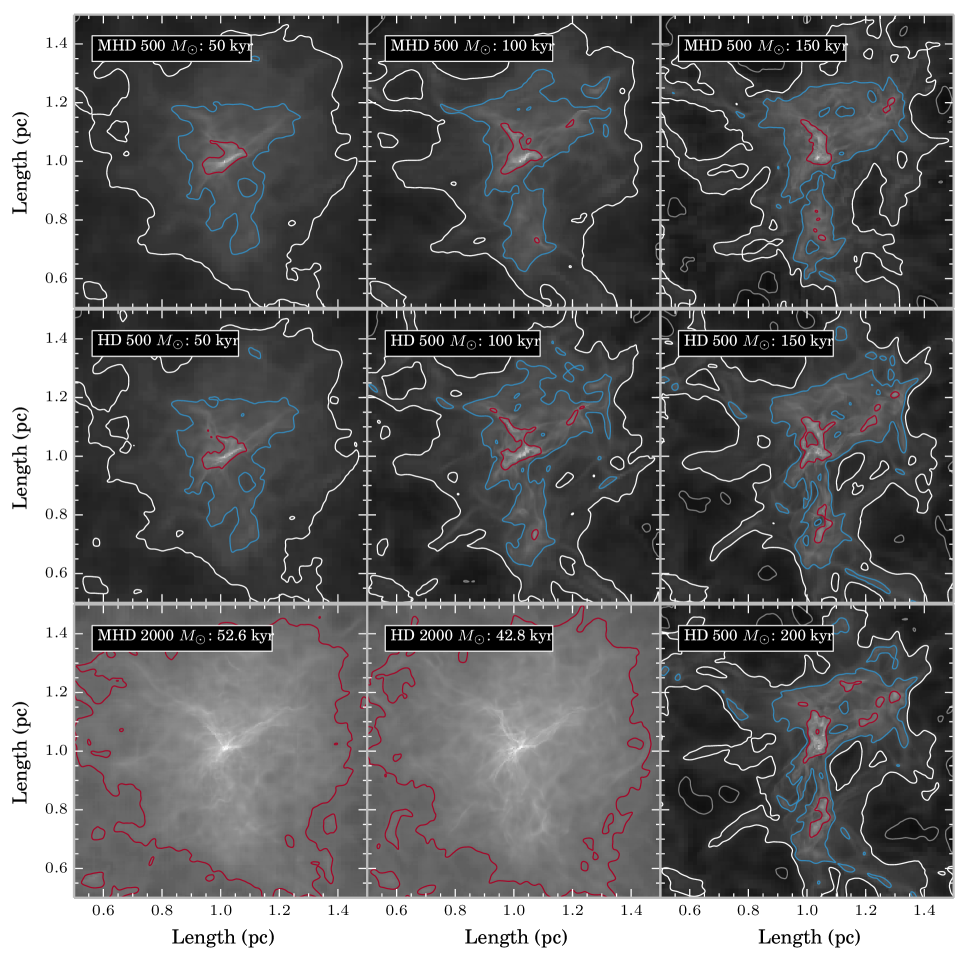
The initial turbulent velocity field quickly results in a highly filamentary structure, as illustrated in Figure 1. We run each of our simulations until the filamentary structure is well-developed; the simulation is stopped at 0.2 to 0.3 free-fall times for the 500 M ${}_{\odot}$ simulations (for the MHD and HD simulations respectively), and 0.13 free-fall times for the 2000 M ${}_{\odot}$ simulations. As flash is an adaptive mesh refinement (AMR) code, we first take the output files and map them to a uniform grid, downsampling somewhat to allow the entire grid to fit into memory. Even with the downsampling, our resolution is $\sim$ 0.002 pc, much better than achievable with Herschel for nearby star-forming regions. We then project the density along each of the coordinate axes to create column density maps.

Figure 1 shows the column density in the X projection for both the 500 M ${}_{\odot}$ and 2000 M ${}_{\odot}$ simulations at all time steps analyzed. Note that the MHD simulation was run for 0.15 Myr, while the HD simulation was run for 0.2 Myr for the 500 M ${}_{\odot}$ simulations, giving one additional time step for our HD analyses. In this figure, all the panels have the same dynamic range shown for the greyscale column density, highlighting that material accumulates into filamentary structures quite quickly (top and middle panel from left to right), and that having an initially higher density more rapidly leads to dense filamentary structures due to the increased importance of gravity (bottom row, left and middle panels). Finally, the presence of a magnetic field acts to slow the accumulation of material into dense filaments, as can be seen comparing the top and middle row panels, or the bottom row left and middle panels. We will return to this point in more detail in Section 3 and beyond.

To extract the filamentary structure evident in Figure 1 , we use the DisPerSE filament-finding algorithm¹¹1http://www2.iap.fr/users/sousbie/ described in Sousbie1 and Sousbie2. The DisPerSE algorithm identifies persistent topological structures such as peaks, voids, and filaments, and is effective even if the image is noisy. It has been extensively used on Herschel observations for filamentary structure identification, e.g. Arzoumanian11; Schneider12; Peretto+2012; Palmeirim13. In DisPerSE, there are several user-defined parameters to control the resulting filamentary network: persistence and robustness thresholds, smoothing, and a maximum angle. The two thresholds can be thought of as very roughly corresponding to criteria for a minimum absolute brightness (persistence threshold) and a minimum relative brightness compared to neighbouring features (robustness threshold). Smoothing removes small-scale ‘wiggles’ from the initial filament spine, while the angle is used to specify the minimum angular rotation between two initial filament spine segments that can be joined together and still be classified as the same filament. Filament spine segments which meet at a right angle, for example, are likely not part of the same filament.

Refer to caption — Figure 1.— A comparison of the column density distribution projected along the X axis for the simulations. The top two rows show the 500 M ${}_{\odot}$ simulations at 0.05, 0.1, and 0.15 Myr after the start of the simulation (left to right) for the MHD (top) and HD (middle) runs. The bottom row shows the MHD and HD 2000 M ${}_{\odot}$ simulations at 0.05 Myr (left and middle) and the HD 500 M ${}_{\odot}$ simulation at 0.2 Myr (right). All simulations are shown cropped to the inner 1.5 pc to better show the smaller-scale structure that forms. The greyscale range is the same in all panels, going from 0.01 to 10 g cm ${}^{-2}$ ( $\sim 3\times 10^{21}$ to $3\times 10^{23}$ cm ${}^{-2}$ ) from black to white, with a logarithmic scaling applied. The overlaid contours show column densities of 0.02, 0.04, 0.075, and 0.2 g cm ${}^{-2}$ (5.3, 1.1, 2.1, and 53 $\times 10^{21}$ cm ${}^{-2}$ ) in grey, white, blue, and red, respectively. If several assumptions are made, including that all pixels belong to cylindrical structures with a characteristic width of 0.1 pc, then the contours also correspond to mass per unit length values 0.5, 1, 2, and 5 times the critical mass per unit length at a temperature of 10 K (18 M ${}_{\odot}$ pc ${}^{-2}$ ). Note that these assumptions are poor for regions not associated with filamentary structure. See Section 3.4 for more detail.

We identify filaments using a persistence threshold of 0.025 g cm ${}^{-2}$ and a robustness threshold of 0.05 g cm ${}^{-2}$ in the 500 M ${}_{\odot}$ simulation (or 7 and 14 $\times 10^{21}$ cm ${}^{-2}$ ) and thresholds of 0.1 g cm ${}^{-2}$ and 0.2 g cm ${}^{-2}$ (or 2.8 and 5.6 $\times 10^{22}$ cm ${}^{-2}$ ) respectively for the 2000 M ${}_{\odot}$ simulation, smoothing the resulting filaments 1000 times, and allowing the initially identified filament segments to be connected for angles of less than 60 degrees (relative to a straight line). These parameters were chosen after testing a range of values to determine which values produced a filamentary structure that best matched visually-apparent structures. All of these thresholds for DisPerSE are above the standard ‘threshold for star formation’ found in nearby molecular clouds of around $\sim 5-7\times 10^{21}$ cm ${}^{-2}$ (e.g., Johnstone04; Konyves13). Unlike the Herschel analyses, we applied DisPerSE directly on the column density map. Since our column density maps include only the gas from the simulated star-forming clump, with no potential contribution from other dense structures within the larger cloud, we have less need than with Herschel data to apply filament-enhancing algorithms. Finally, we excluded several very short filaments that DisPerSE initially identified - in order to accurately determine the filament profile (below), we set a minimum length of 0.1 pc.

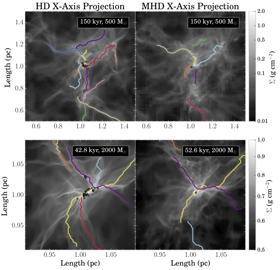
Figure 2 shows the network of filaments identified in the X projection of the 500 M ${}_{\odot}$ and 2000 M ${}_{\odot}$ HD simulations overlaid on their column density maps.

One of the goals of our analysis is to track the time evolution of and the effect of magnetic fields on individual filaments. In order to do so, DisPerSE was not used to identify a different network of filaments at every time step and magnetic field value, as this could potentially lead to different filaments being identified at different snapshots. Instead, for each of the three projections, we started with the network of filaments identified with DisPerSE at 0.15 Myr in the HD simulation, and then searched for the corresponding structures at different times and with magnetic fields present. For the 2000 M ${}_{\odot}$ simulations, we instead started with the single 0.05 Myr time step. We started with an automated procedure to identify equivalent filaments at other time steps and / or with magnetic fields, by searching for local column density maxima near the reference set of filament spines. After this step, all filament spines were verified and adjusted as necessary by hand, using a combination of visual inspection of the current column density snapshot and a movie of the time evolution of the column density map for the 500 M ${}_{\odot}$ simulations. The simulations, particularly without the moderating presence of magnetic fields, form significant substructure on all scales, making it difficult to impossible for an automated procedure to correctly ‘follow’ the filaments in time and across initial conditions.

There are several cases where a filament could not be fully traced to earlier times or in the corresponding simulation with magnetic fields. Some, but not all, of these cases appear to be attributable to structures which are only apparent as filaments in 2D due to a coincidence of independent 3D structures; at other time steps, the real 3D structures have moved by different amounts and no longer appear connected. We include these structures in our analysis where they do appear as a single filamentary structure, as any real observation which only has column density information is fallible to the same line of sight coincidence confusion. We will address the full 3D nature of filaments in these simulations in an upcoming paper.

A comparison of Figure 1 and Figure 2 shows that the filamentary network identified lies only in the very densest part of the cloud, where the estimated mass per unit length value is signficantly above the thermal critical value (white contours in Figure 1). We will return to this point further in Sections 3.2 and 3.3.

2.3. Calculating Radial Column Density Profiles

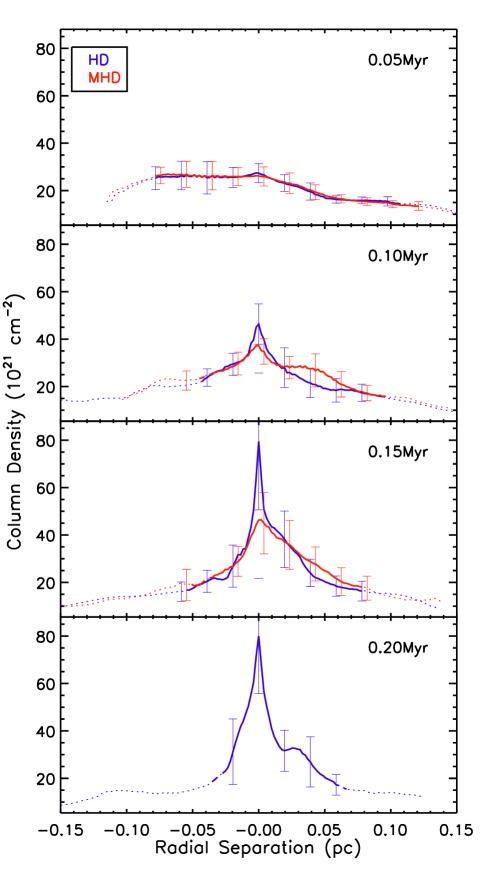
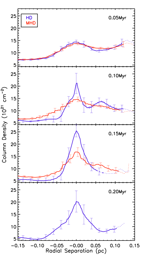
Once the filaments are identified, we measure the radial column density profiles along them. Since the filaments tend to converge toward the simulation centre, and sometimes even intersect, care is needed to properly calculate the radial column density profile. First, we assign every pixel to the filament which it is closest to. Next, we exclude pixels which lie very close ( $<0.01$ pc) to two or more filaments – this value was chosen to provide a balance between not including too many locations which might provide non-representative measures of a given filament profile, and not excluding too large a fraction of material around the filaments. We then calculate the mean column density of pixels in separation bins equal to the pixel size ( $\sim 0.002$ pc). Finally, to ensure that the filament profiles are accurate, we exclude the measurement for any radial bin where at least 25% of the total length of the filament, at that separation, was not included in the profile calculation. This final criterion ensures that all radial column density profile measurements used in our analysis are reliable - there are no cases where data from only a few pixels are used to infer the filament’s properties. We note that the above restrictions limit our analysis to a smaller range in radii than used in Smith14, although the range is closer to Arzoumanian11. Smith14 analyze only the brightest one or two filaments in any given simulation snapshot, which ensures that the contamination in filament profiles will be minimal; with our inclusion of fainter filaments, only smaller radial separations from a given filament spine are free from material from neighbouring filaments. Figures 3 and 4 show several example radial column density profiles which will be further discussed in Section 4.

3. Basic Filament Properties

Visual inspection of the resulting radial column density profiles (e.g., Figures 3 and 4) reveals a variety of characteristics. We expect that after the first turbulent shocks form a filamentary structure, gravity acts to continue to concentrate mass onto these filaments, leading to higher and narrower peaks with time. An initially higher mean density should increase gravity’s pull and lead to a faster filament evolution. The presence of a magnetic field should cushion the initial turbulent compressions, reducing the amount of material initially in the filament, and giving the appearance of ‘fluffier’ filaments. The subsequent evolution of MHD filaments should then be slowed relative to the HD case by gravity’s weaker pull on the the initial lower concentration of mass, and possibly also further action by the magnetic field, depending on its orientation.

Broadly, these behaviours do hold – the visual impression from watching movies of each simulation suggest this behaviour, nevertheless, we find instances of filaments dissipating over time, suggesting gravity was insufficient to prevent the initial turbulent compression from re-expansion. In some of these cases, magnetic fields appear to help to slow or prevent this re-expansion, causing the HD filament to have a higher and narrower peaked profile than in the MHD case. In other instances, data excluded for one or more of the reasons mentioned above (difficulty in tracing the filament, or exclusion due to unreliability) also prevents the full influence of time or magnetic fields to be fully assessed.

Despite this more complex behaviour, there are still several simple measures that we can make to gain insight into the behaviour observed.

3.1. Filament Widths

The conceptually simplest measureable filament property is its width. Although filament widths measured with Herschel span at least a factor of five (e.g., Figure 7 in Arzoumanian11), it is often stated that filaments have a constant width of $\sim$ 0.1 pc. Note, however, that Juvela12b find a larger scatter in filament FWHM values in their analysis of (different) Herschel data, although some of their filaments are much more massive and / or more distant than the Arzoumanian11 sample. We measure the width of all of the filaments tracked in our simulations in the simplest possible method – the extent of the radial profile at half of the peak value, i.e., the FWHM. Table 2 shows our results, separated by time step, magnetic field, and mass. Included is the mean and standard deviation of FWHM values measured, along with the number of FWHM values considered. Some filaments did not have reliable radial column density profiles out to sufficiently large radial separations to allow the FWHM to be measured; these were excluded from the values given in Table 2.

Table 2Filament FWHM values

Mass	Time	HD - FWHM stats ${}^{a}$		MHD - FWHM stats ${}^{a}$		HD - FWHM stats ${}^{b}$		MHD - FWHM stats ${}^{b}$
(M ${}_{\odot}$ )	(Myr)	mean(pc)	stddev(pc)	mean(pc)	stddev(pc)	mean(pc)	stddev(pc)	mean(pc)	stddev(pc)
500	0.05	0.212	0.132	0.262	0.164	0.211	0.127	0.268	0.175
500	0.10	0.105	0.086	0.176	0.130	0.066	0.051	0.116	0.087
500	0.15	0.079	0.073	0.130	0.090	0.050	0.028	0.104	0.051
500	0.20	0.058	0.047	N/A	N/A	0.044	0.025	N/A	N/A
2000	0.05	0.119	0.113	0.168	0.147	0.132	0.137	0.170	0.142

${}^{a}$ All measureable filaments included. ${}^{b}$ Only filaments where the FWHM could be measured at all times in HD and MHD were included. Note that the 500 M ${}_{\odot}$ and 2000 M ${}_{\odot}$ filaments are different samples.