Quantum Critical Scaling of Dirty Bosons in Two Dimensions

Abstract

We determine the dynamical critical exponent, $z$, appearing at the Bose glass to superfluid transition in two dimensions by performing large scale numerical studies of two microscopically different quantum models within the universality class; The hard-core boson model and the quantum rotor (soft core) model, both subject to strong on-site disorder. By performing many simulations at different system size, $L$, and inverse temperature, $\beta$, close to the quantum critical point, the position of the critical point and the critical exponents, $z$, $\nu$ and $\eta$ can be determined independently of any prior assumptions of the numerical value of $z$. This is done by a careful scaling analysis close to the critical point with a particular focus on the temperature dependence of the scaling functions. For the hard-core boson model we find $z=1.88(8)$, $\nu=0.99(3)$ and $\eta=-0.16(8)$ with a critical field of $h_{c}=4.79(3)$, while for the quantum rotor model we find $z=1.99(5)$, $\nu=1.00(2)$ and $\eta=-0.3(1)$ with a critical hopping parameter of $t_{c}=0.0760(5)$. In both cases do we find a correlation length exponent consistent with $\nu=1$, saturating the bound $\nu\geq 2/d$ as well as a value of $z$ significantly larger than previous studies, and for the quantum rotor model consistent with $z=d$.

Most familiar quantum critical points (QCP’s) are characterized by Lorentz invariance implying a symmetry between correlations in space and time and consequently also between the respective correlation lengths $\xi\sim\xi_{\tau}$. In turn, this implies that the dynamical critical exponent, defined through $\xi_{\tau}\sim\xi^{z}$, is simply $z=1$ although $\xi$ and $\xi_{\tau}$ typically differ by an overall pre-factor. Systems for which $z\neq 1$ are comparatively less common and possess a distinct anisotropy between space and time since $\xi$ and $\xi_{\tau}$ are not only different but now also scale differently. One model for which it is generally believed that $z\neq 1$ is the Bose glass to super fluid (BG-SF) transition describing interacting bosons subject to disorder, the so called dirty-boson problem, modelled by the hamiltonian:

$$H_{bh}=-t\sum_{{\mathbf{r}},\bf e}\left(b^{\dagger}_{{\mathbf{r}}}b_{{\mathbf{r}}+\bf e}+h.c.\right)-\sum_{{\mathbf{r}}}\mu_{{\mathbf{r}}}\tilde{n}_{{\mathbf{r}}}+\frac{U}{2}\sum_{{\mathbf{r}}}\tilde{n}_{{\mathbf{r}}}\left(\tilde{n}_{{\mathbf{r}}}-1\right).$$ (1)

Here ${\bf e}={\bf x,y}$, and $b^{\dagger}_{{\mathbf{r}}},b_{\bf r}$ are the boson creation and annihilation operators at site ${\mathbf{r}}$ with $\tilde{n}_{{\mathbf{r}}}$ the corresponding number operator. The parameters of the model are the hopping constant $t$, Hubbard repulsion $U$, and site-dependent chemical potential $\mu_{\mathbf{r}}$, inducing the disorder.

Experimental setups emulating dirty boson physics include optical lattices Greiner et al. (2002); *Pasienski10 adsorbed Helium in random media Crowell et al. (1997), Josephson-junction arrays van der Zant et al. (1992), thin-film superconductors Haviland et al. (1989); *Jaeger89; *Liu91; *Markovic98; *Lin2011 as well as quantum magnets such as doped-DTN Yu et al. (2010); *Rong12nature; *Rong12. For recent reviews see Ref. Zheludev and Roscilde (2013); Weichman (2008).

The dynamical critical exponent, $z$, appearing at the BG-SF transition has proven exceedingly hard to determine. Initial theoretical work Fisher and Fisher (1988); *Fisher90; *Fisher89 argued that $z=d$ in any dimension. This has intriguing implications since it implies the absence of an upper critical dimension, although a scenario involving a discontinuous onset of mean field behavior has beeen proposed Dorogovtsev (1980); *Weichman89; *Mukhopadhyay96. Subsequent numerical studies Krauth et al. (1991); *Runge92; *Batrouni93; Sørensen et al. (1992); *Wallin94; Zhang et al. (1995); Kisker and Rieger (1997); Prokof’ev and Svistunov (2004); Pollet et al. (2009); *Gurarie09; *Carleo13; *Lin11 of the system in two dimensions were consistent with $z=d=2$ and the phase-diagram is well understood Bernardet et al. (2002); *Sengupta07; *Soyler11. More recently, the transition in three dimensions has been investigated both numerically Hitchcock and Sørensen (2006); *Gurarie09; *Yao14 and experimentally White et al. (2009), yielding evidence for $z=d=3$. However, the majority of these numerical studies were not unbiased since implicit assumptions about $z$ are needed to fix the aspect ratio $L^{z}/\beta$ in the simulations.

The arguments leading to the equality $z=d$ starts with hyperscaling Stauffer et al. (1972); *Aharony74; *Hohenberg76 which states that the singular part of the free energy inside a correlation volume is a universal dimensionless number, $(f_{s}/\hbar)\xi^{d}\xi_{\tau}=A.$ With $\xi\sim\delta^{-\nu}$ it follows that $f_{s}\sim\delta^{\nu(d+z)}$ with a finite-size form: Fisher et al. (1989)

$$f_{s}(\delta,L,\beta)\sim\delta^{\nu(d+z)}F(\xi/L,\xi_{\tau}/\beta).$$ (2)

Imposing a a phase gradient $\partial\phi$ along one of the spatial directions will then give rise to a free energy difference $\Delta f_{s}/\hbar=\frac{1}{2}\rho(\partial\phi)^{2}$ where $\rho$ is the stiffness (superfluid density). Since $\Delta f_{s}$ must obey a form similar to Eq. (2) and since $\partial\phi$ has dimension of inverse length implying $\partial\phi\sim 1/\xi$, it follows that $\rho\sim\xi^{2}\delta^{\nu(d+z)}\sim\delta^{\nu(d-2+z)}$, with a finite-size scaling form of:

$$\rho=L^{d-2-z}R(\delta L^{1/\nu},\beta/L^{z}),$$ (3)

Following Ref. Fisher et al., 1989, an analoguous argument imposing a twist in the temporal direction leads to $\Delta f_{s}/\hbar=\frac{1}{2}\kappa(\partial_{\tau}\phi)^{2}$ and $\kappa\sim\xi_{\tau}^{2}\delta^{\nu(d+z)}\sim\delta^{\nu(d-z)}$ assuming $\partial_{\tau}\phi\sim 1/\xi_{\tau}$. On the other hand, if $\delta=(\mu-\mu_{c})$, the singular part of the compressibility $\kappa_{s}$ must from Eq. (2) obey $\kappa_{s}\sim\delta^{\nu(d+z)-2}$. Assuming that $z>d$, so that $\kappa$ diverges, it follows that $\kappa=\kappa_{s}$ which leads to $z\nu=1$. With $z>d$ this result would then contradict the (quantum) Harris inequality $\nu\geq 2/d$ Chayes et al. (1986) invalidating the initial assumption. Hence, one must have $z\leq d$. Finally, if one argues that for the disordered system $\kappa$ cannot vanish at criticality the relation $\kappa\sim\delta^{\nu(d-z)}$ implies $z=d$.

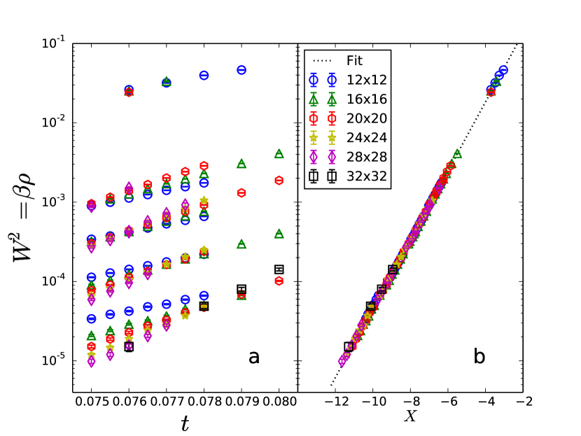
Figure 1: (Color online) Scaling collapse of 142  independent simulations of $W^{2}=\beta\rho$ for the QR model. (a) Unscaled data of $W^{2}$ versus $t$ for $L=12,\ldots,32$. (b) Scaling collapse of the data of panel (a). The data is plotted against the scaling variable $X=\ln(a\beta/L^{z})+b(t-t_{c})L^{1/\nu}-cL/\beta^{1/z}-d(L/\beta^{1/z})^{2}$ obtaining $z=1.99(5)$, $\nu=1.00(2)$, $t_{c}=0.0760(5)$.

More recent theoretical work Weichman and Mukhopadhyay (2007); *Weichmanprb08; Weichman (2008) has questioned the arguments leading to the equality $z=d$. In particular, in the presence of disorder breaking particle-hole symmetry, it was argued Weichman and Mukhopadhyay (2007); *Weichmanprb08 that $\kappa-\kappa_{s}$ is dominated by the analytical background and $\partial_{\tau}\phi\sim 1/\xi_{\tau}$ should not apply, invalidating the relation $\kappa\sim\delta^{\nu(d-z)}$, leaving $z$ unconstrained. A recent numerical Priyadarshee et al. (2006) study of the hard-core version of Eq. (1) finds $z=1.4\pm 0.05$, by analyzing scaling behavior of quantities relatively far from criticality. However, in that study, relatively few disorder realizations ($10-10^{3}$) were used and the location of the QCP was not reliably determined. In more recent work, Meier et al Meier and Wallin (2012) performed a state of the art calculation of a soft-core version of Eq. (1) finding a significantly larger value of $z=1.75\pm 0.05$ and $\nu=1.15(3)$. While the location of the QCP was determined with an impressive precision this latter study does not employ a fully quantum mechanical model but instead uses an effective classical model for which the temperature dependence, at the heart of the scaling with $z$, is only approximately accounted for. It is for instance not possible to calculate the specific heat of the underlying quantum model using the representation of Meier and Wallin (2012).

At present, the value of $z$ at the dirty-boson QCP along with many of the other exponents most notably $\nu$ can therefore best be regarded as ill determined, at least for the fully quantum mechanical model. It is not known to what extent, if any, the relation $z=d$ is violated nor if the relation $\nu\geq 2/d$ Chayes et al. (1986) is obeyed, although, as outline above it seems reasonable to expect $z\leq d$ if indeed the inequality $\nu\geq 2/d$ is obeyed and, as shown in Fisher et al. (1989), $z\geq 1$ in any dimension. Here we try to answer these questions by performing large-scale simulations on two fully quantum mechanical models; A hard-core boson model (HCB) modelled as a transverse field $XY$ model and a soft-core quantum rotor model (QR), both of which are subject to strong on-site disorder. In all cases do we use $10^{4}-10^{5}$ disorder realizations over a large range of temperatures extending down to $\beta=1024$ for linear system sizes $L=12-32$.

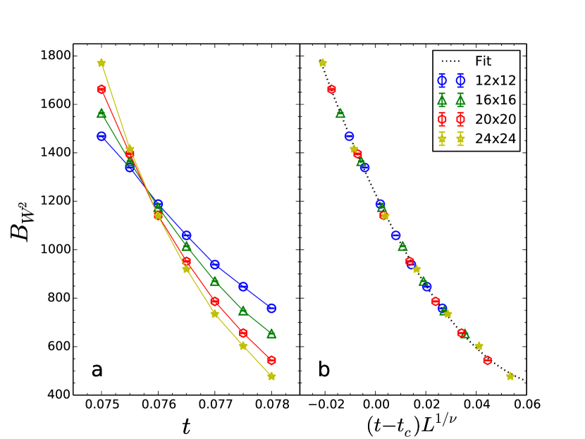
Figure 2: (Color online) The Binder cumulant $B_{W^{2}}$ for the QR model versus $t$ with $\beta=L^{2}/4$. (a) Unscaled data showing a crossing close to the critical point $t_{c}=0.0760(5)$. (b) Scaling plot versus $(t-t_{c})L^{1/\nu}$ obtained by fitting the data in (a) to the form $a+b(t-t_{c})L^{1/\nu}+c(t-t_{c})^{2}L^{2/\nu}$ yielding $t_{c}=0.758(5)$ and $\nu=0.98(3)$.

Models: The first model we study, closely related to Eq. (1), is the quantum rotor (QR) model. It is defined in terms of conjugate phase and number operators $\theta_{\mathbf{r}},n_{\mathbf{r}}$ satisfying $[\theta_{\mathbf{r}},n_{{\mathbf{r}}^{\prime}}]=\delta_{{\mathbf{r}},{{\mathbf{r}}^{\prime}}}$ on a $L\times L$ lattice:

$$H_{\text{qr}}=-\sum_{{{\mathbf{r}}},{{\mathbf{r}}+\bf e}}t\cos(\theta_{\bf r}-\theta_{\bf r+e})-\sum_{\bf r}\mu_{\bf r}n_{\mathbf{r}}+\frac{U}{2}\sum_{\bf r}n^{2}_{\mathbf{r}}\,$$ (4)

where $U$ is the onsite repulsion, $t$ is the nearest neighbor tunneling amplitude and $\mu_{r}\in[-\Delta,\Delta]$ represents the uniformly distributed on-site disorder in the chemical potential. As before, ${\bf e}={\bf x,y}$. The disorder for a given disorder realization is not constrained and in all simulations we use $\Delta=\frac{1}{2}$, $U=1$ and tune through the BG-SF transtion varying $t$ at constant $\Delta$. In contrast to Eq. (1) $n_{\mathbf{r}}$ can take negative as well as positive values and one can loosely associtate $n_{\mathbf{r}}$ with deviations from the average filling $n_{0}$ in Eq. (1), $\tilde{n}_{\mathbf{r}}-n_{0}$. For convenience we study Eq. (4) using a link-current representation Witczak-Krempa et al. (2014) for which directed worm algorithms are available Alet and Sørensen (2003a); *Aletb. We use lattice ranging from $L=12$ to $L=32$, with 50,000 disorder realizations for $L=12,\ldots,28$ and 10,000 disorder realizations for $L=32$ in all cases with $6\times 10^{4}$ MCS  per disorder realization. For the simulations of the QR model a temporal discretization of $\Delta\tau=0.1$ was used, sufficiently small that remaining discretization errors could be neglected.

The second model we consider is the $U\to\infty$ hard-core limit of Eq. (1) where the boson occupation number is constrained to $0,1$. It is therefore therefore equivalent to the following $S=1/2$ $XY$-model on a $L\times L$ lattice in a random transverse field:

$$H_{xy}=-\frac{1}{2}\sum_{{\mathbf{r}},\bf e}\left(S^{+}_{{\mathbf{r}}}S^{-}_{{\mathbf{r}}+\bf e}+S^{-}_{{\mathbf{r}}}S^{+}_{{\mathbf{r}}+\bf e}\right)+\sum_{\mathbf{r}}h_{\mathbf{r}}S^{z}_{\mathbf{r}},$$ (5)

where $h_{\mathbf{r}}\in\left[-h,h\right]$ uniformly. In this case we tune through the transition by increasing the disorder strength, $h$. Despite the representation as a spin model, we shall refer to this as the hard-core boson model (HCB). We use a directed loop version of the stochastic series expansion (SSE) Sandvik and Kurkijärvi (1991); *Olav02 to simulate this model. This technique does not have discretization errors and efficient directed algorithms Syljuåsen and Sandvik (2002); Alet et al. (2005) are available. For the SSE calculations, we use a beta-doubling scheme Sandvik (2002) that allows us to very quickly equilibrate at large $\beta$ values. For each temperature in the beta-doubling scheme, we average over $48$ Monte Carlo sweeps (MCS), with each sweep consisting of one diagonal update and $N_{l}$ directed loop updates. $N_{l}$ is set during the equilibration phase so that on average $2\langle n_{H}\rangle$ vertices are visited, where $n_{H}$ is the number of non-trivial operators in the SSE string. In contrast to the QR model, we use here a microcanonical ensemble for the disorder by constraining each disorder realization to have exactly $\sum h_{\mathbf{r}}=0$. This facilitates the analysis and is not believed to affect the results Dhar and Young (2003); *Monthus04. We use at least $\sim 10^{5}$ disorder realizations per data point, a large improvement over Priyadarshee et al. (2006).

In the following $[\ldots]$ denotes the disorder average while $\left<\ldots\right>$ denotes the thermal average. In simulations of both models two independent replicas $\alpha,\beta$ of each disorder realization are simulated in parallel so that combined averages $[\left<\ldots\right>^{2}]$ may be correctly estimated as $[\left<\ldots\right>_{\alpha}\left<\ldots\right>_{\beta}]$.

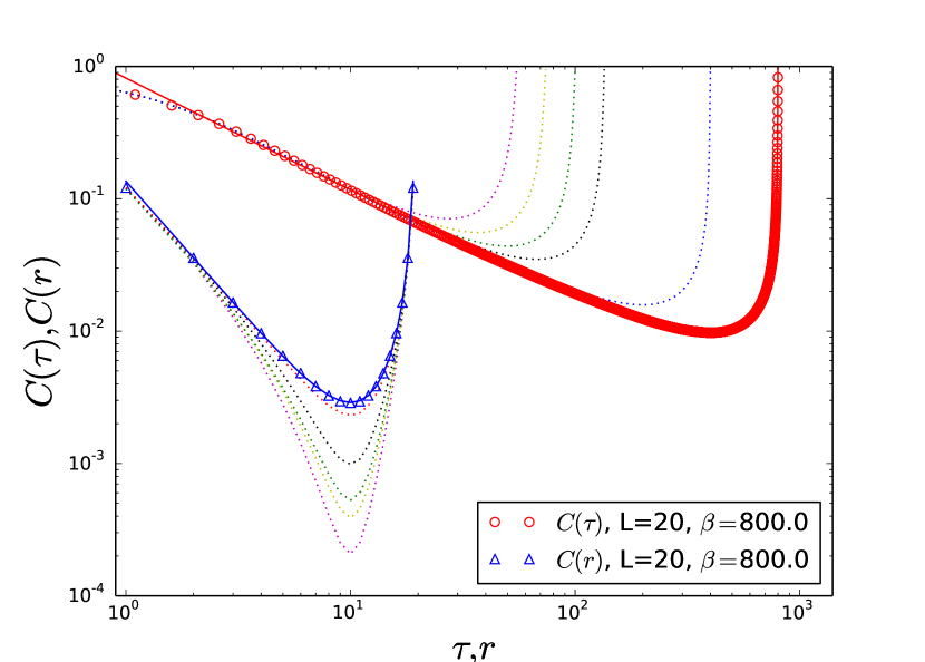
Figure 3: (color online) The correlation functions $C(\tau)$ and $C({\bf r})$ as a function of $\tau,{\bf r}$ for a system size $L=20$. Results are shown for the QR model at the critical point and a range of $\beta=55,\ldots,800$. The solid red line is a fit to $\beta=800$ results for $C(\tau)$ using the form $a(\tau^{-y_{\tau}}+(\beta-\tau)^{-y_{\tau}})$ with $(z+\eta)/z$=$y_{\tau}=0.85(2)$.

Observables: Our main focus is the scaling behaviour of the superfluid stiffness, $\rho$, for which the finite-size scaling form Eq. (3) was derived. For both models we measure $\rho$ as:

$$\rho=\frac{[\left<W_{x}^{2}+W_{y}^{2}\right>]}{2\beta},$$ (6)

where $W_{x}$ and $W_{y}$ are the winding numbers in the spatial directions. (For the HCB model Eq. (6) is multiplied by $\pi$ to yield $\rho$.) From Eq (6) it follows that $\beta\rho=W^{2}$ has a particularly attractive scaling form when $d=2$, which we may write:

$$W^{2}=\frac{\beta}{L^{z}}W(\delta L^{1/\nu},L/\beta^{1/z}),$$ (7)

where we define $\delta=(t-t_{c})$ (QR model) and $\delta=(h-h_{c})$ (HCB model). We also make extensive use of the correlation functions, defined as $C({\mathbf{r}}-{\mathbf{r}}^{\prime},\tau-\tau^{\prime})=[\left<\exp(i(\theta_{\mathbf{r}}(\tau)-\theta_{{\mathbf{r}}^{\prime}}(\tau^{\prime})))\right>]$ for the QR model and as $C({\mathbf{r}}-{\mathbf{r}}^{\prime},\tau-\tau^{\prime})=[\left<S^{+}_{\mathbf{r}}(\tau),S^{-}_{{\mathbf{r}}^{\prime}}(\tau^{\prime})\right>]$ for the HCB model.

Results, QR: A large number of independent simulations of Eq. (4) were carried out at different $L=12,\ldots,32$ and $\beta=20,\ldots,400$ close to the QCP. Since we expect $\rho$ to approach zero in an exponential manner as $L$ is increased at fixed $\beta$ and since $\rho$ is likely exponentially suppressed in the insulating phase it seems reasonable to approximate the function $W(x,y)$ in Eq. (7) as $a\exp(f(x,y))$ with $x=\delta L^{1/\nu},\ y=L/\beta^{1/z}$. If the temperature dependence is carefully mapped out Sup one indeed sees that $W(x,y)$ has a clear exponential dependence. As a first step, we then assume $f(x,y)=bx-cy-dy^{2}$. We can then fit all 142  data points to this form determining the coefficients $a,b,c,d$ along with $t_{c}=0.0760(5)$  $\nu=1.00(2)$ and $z=1.99(5)$. The results are shown in Fig. 1 with a scaling plot using the scaling variable $X=\ln(a\beta/L^{z})+b(t-t_{c})L^{1/\nu}-cL/\beta^{1/z}-d(L/\beta^{1/z})^{2}$. A more refined analysis Sup shows that the temperature dependence likely involves a correction term $W^{2}=ay^{z}\exp(bx-cy)+dy^{-w}\exp(bx-c^{\prime}y)$. The correction term is here proportional to $T^{w}$ and disappears as $T$ tends to zero. It is straight forward to fit all our data to this form which yields identical estimates for $t_{c},\nu$, $z$ along with $w=0.6(2)$. Estimating the AIC (Akaike Information Criterion) for the two forms heavily favors the latter.

With a reliable estimate of $z$ we can fix the scaling argument $L^{z}/\beta$ by appropriately selecting $\beta$ for each $L$. If we then study the Binder cumulant $B_{W^{2}}=[\left<W^{4}\right>]/[\left<W^{2}\right>]^{2}$ we see that at fixed $L^{z}/\beta$ it should follow a simplified form of Eq. (7), $B_{W^{2}}=B(\delta L^{1/\nu})$. As shown in Fig. 2, lines for different $L$ will then cross at $t_{c}$. This is indeed the case, confirming our previous estimates.

Our results for the correlation functions for the QR models are shown in Fig. 3 for a $L=20$ lattice at $t_{c}$ for a range of temperatures. Asymptotically, one expects Fisher et al. (1989) $C(\tau)\sim\tau^{-(d+2-z+\eta)/z}$ and $C({\mathbf{r}})\sim r^{-(d+2-z+\eta)}$. Clearly, $C({\mathbf{r}})$ drops off much faster than $C(\tau)$ confirming that $z\neq 1$. However, pronounced finite temperature effects are visible in $C({\mathbf{r}})$ arising because the limit $\beta\gg L^{z}$ has not yet been reached and we have not been able to reliable determine the power-law describing $C({\mathbf{r}})$. However, from $C(\tau)$ we determine $(z+\eta)/z$=$y_{\tau}=0.85(2)$ and hence $\eta=-0.3(1)$ using our previous estimate $z=1.99(5)$.

For the QR model we have also verified that the compressibility, $\kappa$, remains finite and independent of $L$ throughout the transition, consistent with $z\leq d$. Furthermore, a direct evaluation of $\frac{\partial W^{2}}{\partial t}$ directly at $t_{c}$ for fixed $L^{z}/\beta$, expected from Eq. (7) to scale as $\sim L^{1/\nu}$, yields $\nu=0.98(4)$ consistent with our previous results.

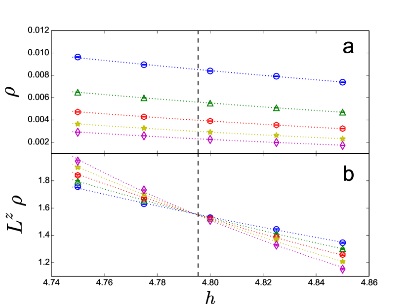
Figure 4: (Color online) Finite-size scaling analysis of the stiffness for the HCB model using data only at $\beta=512$. (a) $\rho$ vs $h$ for system sizes: $L=16,20,\dots 32$. (b) Crossing of the scaling function: $\tilde{R}=L^{z}\rho$ at the critical point: $h_{c}=4.79(3)$ (vertical dashed line). For both panels, the dotted lines are second order series expansions of $\tilde{R}(x)=a+bx+cx^{2}$, fitted to the data.

Results, HCB: Due to the hard-core constraint number fluctuations are dramatically suppressed in the HCB model. Combined with the very effective beta-doubling scheme we can effectively reach much lower temperatures with the HCB model relative to the QR model. Hence, we use a simplified form of Eq. (3):

$$\rho=L^{d-2-z}\tilde{R}(\delta L^{1/\nu}),$$ (8)

suppressing the temperature dependence. We have extensively verified that this is permissible for the system sizes used Sup and that our data appear independent of temperature at $\beta=512$ to within numerical precision. We then fit our data for $\rho$ at $\beta=512$ to an expansion of $\tilde{R}$ in Eq. (8) to second order: $\tilde{R}=a+b\delta L^{1/\nu}+c(\delta L^{1/\nu})^{2}$ obtaining the estimates: $h_{c}=4.79(3)$, $z=1.88(8)$, $\nu=0.99(3)$. The result of this fit is shown in Fig. 4, where our simulation data (unfilled markers) is superimposed with the quadratic fit (dotted lines). In panel $b$ of Fig. 4, we show the crossing of the scaling function $\tilde{\rho}$, at $h_{c}=4.79(3)$. By including all results for $\beta<512$ it is also possible to perform an identical analysis to the one performed for the QR model in Fig. 1. Such an analysis similar results for $z$, $\nu$ and $h_{c}$.

As was the case for the QR model the correlation functions show a pronounced temperature dependence as shown in Fig. 5(a) for $C({\mathbf{r}})$. However, as we lower the temperature, $C({\mathbf{r}})$ reaches a stable power-law form at $\beta=512$ for all $L$ studied showing that the regime $\beta\gg L^{z}$ is reached for all $L$ and confirming that the temperature dependence can be neglected in Eq. (8). To determine the anomalous dimension $\eta$ we then fit the results in Fig. 5(a) for $L=20$, $\beta=512$ $h_{c}=4.79(3)$ to a power-law form with $z+\eta$=$y_{r}=1.718(1)$ as shown in Fig. 5(b). Using our earlier estimate of $z$, we obtain $\eta=-0.16(8)$ in reasonable agreement with the result for the QR model.

For the HCB model we have also calculated the compressibility, $\kappa$. It remains roughly constant and independent of $L$ through the transition.

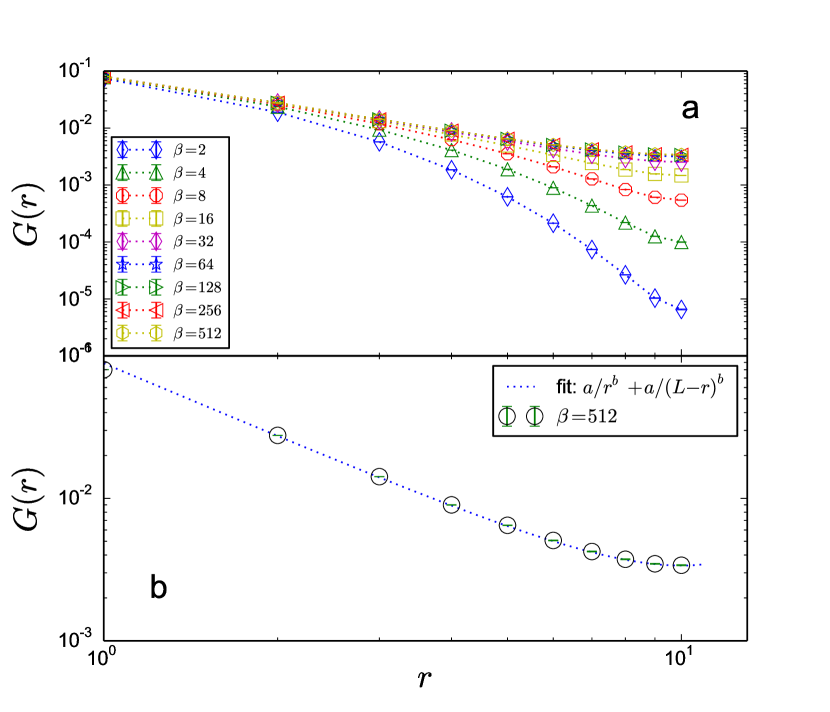
Figure 5: (color online). The equal-time spatial correlation function: $C({\mathbf{r}})$ of a $20\times 20$ lattice for the HCB model at $h_{c}$. (a) Convergence of $C({\mathbf{r}})$ using the beta-doubling procedure. For $L=20$, $C({\mathbf{r}})$ appears independent of $\beta$ for $\beta\geq 128$. (b) $C({\mathbf{r}})$ simulation data (open circles) at $\beta=512$ fitted to the form $a\left(1/r^{y_{r}}+1/(L-r)^{y_{r}}\right)$ (dashed line), yielding $z+\eta=$$y_{r}=1.718(1)$.

Conclusion: Our results for $\nu$ for both models studied indicate clearly that $\nu\geq 2/d$ is satisfied as an equality. For the dynamical critical exponent $z$, describing the BG-SF transition, we find a value that is significantly larger than previous estimates. While there is a slight disagreement in the estimate of $z$ for the two models we studied it seems possible that indeed $z=d$. In light of this it now seems particularly interesting to focus attention on the transition in $d=4$.

During the final stages of writing this manuscript we became aware of Ref. Álvarez Zúñiga et al., 2014 which for the HCB model reach conclusions similar to ours.

I Acknowledgements

Appendix A Supplementary material

A.1 HCB simulation details

A central assumption made in our analysis of the HCB results was that a simplified scaling function, Eq. (8), for $\rho$. In the main text, we showed the convergence of the equal-time spatial correlation function: $C({\mathbf{r}})$ in Fig. 5 at the critical point using data from the beta-doubling procedure. For completeness, we show the convergence of the stiffness in Fig. 6 for a $32\times 32$ lattice. Unlike the $20\times 20$ system, we need to go up to $\beta=512$ before finite temperature effects are eliminated. The data indicates that for the simulation of even larger system sizes, one may need to go up to $\beta=1024$ to validate the use of the simplified scaling form.

Another important point that is often overlooked, is the convergence of observable data with the number of disorder realizations, $N_{r}$ used. For the SSE parameters chosen, we find that it was necessary to use at least $\sim 5\times 10^{4}$ disorder samples before disorder fluctuations are reasonably small. This is demonstrated in Fig. 7 for the largest lattice size: $32\times 32$. For reliable data with controlled errorbars, all the HCB data points were averaged over least $10^{5}$ independent disorder realizations. This is contrast to earlier studies Priyadarshee et al. (2006) most relevant to our work, where only $10^{2}-10^{3}$ disorder realizations were used. We note that it is quite unlikely that self-averaging applies in this model and increasing the lattice size does therefore not decrease the number of disorder realizations needed.

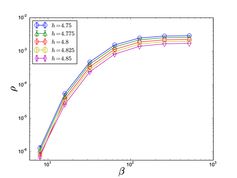
Figure 6: Demonstration of the convergence of the spin stiffness: $\rho$ versus $\beta$ using the beta-doubling procedure, for a $32\times 32$ lattice. As $\beta$ increases, thermal effects can be clearly seen to disappear, thereby justifying the use of the simplified scaling form in Eq. (8).

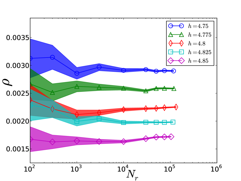
Figure 7: Convergence of spin stiffness: $\rho$ with number of disorder realizations, $N_{r}$, for $h$ values used. The shaded region indicates the errorbars of points which decrease as more samples are used. Note that for the equilibration step size chosen in our simulations, $\sim 10^{5}$ disorder realizations are necessary to obtain true convergence.

Appendix B Temperature dependence of $W^{2}=\beta\rho$

Insight into the temperature dependence of $W^{2}$ can be gained by first studying $\rho$ for the QR model without disorder. A model for which it is know that $z=1$. Results for $\rho$ for a $40\times 40$ lattice are shown in Fig. 8 for $\beta=9,\ldots 400$. For $\beta\ll L$ we expect $\rho$ to go zero in an exponential manner while for $\beta\gg L$ it should approach a constant. The simplest ansatz is therefore:

$$\rho=\frac{a}{L}e^{-c\frac{L}{\beta}},$$ (9)

where we have tentatively included an $L$ dependence. However, as is clearly evident in Fig. 8, $\rho$ has a maximum close to $L/\beta=0.4$. The presence of this maximum signals that there are likely two contributions to $\rho$ describing the $\beta\ll L$ and $\beta\gg L$ regimes. (Although we note that the existence of two terms does not imply a maximum.) We therefore assume the presence of a correction term proportional to $T^{y}$ with $y>0$. Such a term will therefore disappear in the zero temperature limit. For our final ansatz we therefore take:

$$\rho=\frac{a}{L}e^{-c\frac{L}{\beta}}+b\left(\frac{L}{\beta}\right)^{y}e^{-d\frac{L}{\beta}}.$$ (10)

This is the form used in Fig. 8 and it gives an essentially perfect fit over the entire range of the figure. We can immediately generalize to a scaling form for $W^{2}=\beta\rho$:

$$W^{2}=a\frac{\beta}{L}e^{-c\frac{L}{\beta}}+b\left(\frac{L^{z}}{\beta}\right)^{w}e^{-d\frac{L}{\beta}}.$$ (11)

A fit to this form yields $\omega=0.97(9)$ in relative good agreement with similar correction terms used in Ref. Witczak-Krempa et al. (2014).

We now turn to the QR model in the presence of disorder. In this case we assume that the scaling variable $L/\beta$ generalizes to $L/\beta^{1/z}$. We therefore expect to find:

$$W^{2}=a\frac{\beta}{L^{z}}e^{-cL/\beta^{1/z}}+b\left(\frac{L^{z}}{\beta}\right)^{w}e^{-dL/\beta^{1/z}}.$$ (12)

In Fig. 9 results are shown for $W^{2}$ for two different lattice sizes $L=12,20$ Assuming $z=2$ in this case we plot the results against $L/\sqrt{\beta}$ demonstrating that the results fall on a single curve with only slight deviations from a straight line. It is perhaps surprising that it is the variable $L/\beta^{1/z}$ that appears as opposed to $L^{z}/\beta$ but this can very clearly be verified from the simulations. Performing a fit to the ansatz we find exceedingly good agreement with the expected form with a correction exponent $w=0.92(7)$, close to the value for the model without disorder. An inspection of our results for $\rho$ for this system size shows that in this case there is no maximum in $\rho$ versus $\beta$.

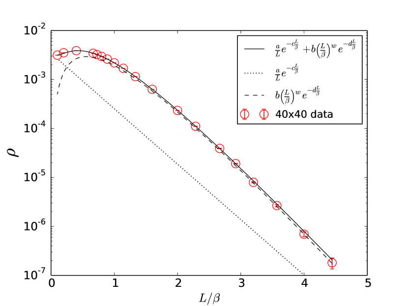
Figure 8: (Color online) $\rho$ as a function of $L/{\beta}$ for the QR model without disorder. Results are shown for $L=40$. The solid black line indicates a fit to the $L=40$ data of the form $\frac{a}{L}e^{-c\frac{L}{\beta}}+b\left(\frac{L}{\beta}\right)^{y}e^{-d\frac{L}{\beta}}$ yielding $y=1.97(9)$. The dotted line indicates the first part of this fit while the dashed line shows the second part.

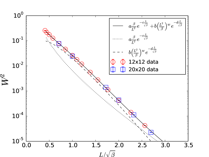
Figure 9: (Color online) $\beta\rho$ as a function of $L/\sqrt{\beta}$ for the QR model. Results are shown for $L=12,20$. The solid black line indicates a fit to the $L=12$ data of the form $a\frac{\beta}{L^{2}}e^{-c\frac{L^{2}}{\beta}}+b\left(\frac{L^{2}}{\beta}\right)^{w}e^{-d\frac{L}{\sqrt{\beta}}}$ yielding $w=0.92(7)$. The dotted line indicates the first part of this fit while the dashed line shows the second part.

We have performed a similar analysis of $W^{2}$ as a function of $\beta$ for the QR model again clearly confirming the overall exponential dependence and the presence of the two terms.

Appendix C Crossing of $\beta\rho$ for the QR model.

With the $z$ and $t_{c}$ determined from the fit in Fig. 1 $\beta\rho$ plotted for different $L$ at a fixed aspect ratio $\beta=L^{z}/4$ should also cross at the critical point $t_{c}=0.0760(5)$. This is indeed the case and is shown Fig. 10. Since this data is essentially already shown in Fig 1(a) we have in the main text opted to show the crossing using the related quantity $B_{W^{2}}=[\left<W^{4}\right>]/[\left<W^{2}\right>]^{2}$ shown in Fig. 2.

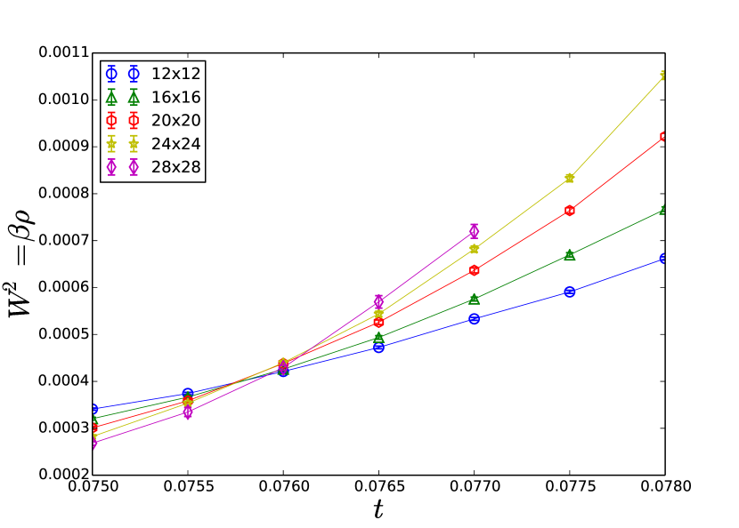
Figure 10: (Color online) $\beta\rho$ as a function of $t$ for the QR model. All simulations are performed using the fixed aspect ratio $\beta=L^{z}/4$ with $z=2$. Lines cross at the critical point $t_{c}=0.0760(5)$.