A CONTINUUM OF SMALL PLANET FORMATION BETWEEN 1 AND 4 EARTH RADII

Abstract

It has long been known that stars with high metallicity are more likely to host giant planets than stars with low metallicity. Yet the connection between host star metallicity and the properties of small planets is only just beginning to be investigated. It has recently been argued that the metallicity distribution of stars with exoplanet candidates identified by Kepler provides evidence for three distinct clusters of exoplanets, distinguished by planet radius boundaries at $1.7\,R_{\oplus}$ and $3.9\,R_{\oplus}$. This would suggest that there are three distinct planet formation pathways for super-Earths, mini-Neptunes, and giant planets. However, as I show through three independent analyses, there is actually no evidence for the proposed radius boundary at $1.7\,R_{\oplus}$. On the other hand, a more rigorous calculation demonstrates that a single, continuous relationship between planet radius and metallicity is a better fit to the data. The planet radius and metallicity data therefore provides no evidence for distinct categories of small planets. This suggests that the planet formation process in a typical protoplanetary disk produces a continuum of planet sizes between $1\,R_{\oplus}$ and $4\,R_{\oplus}$. As a result, the currently available planet radius and metallicity data for solar-metallicity F and G stars give no reason to expect that the amount of solid material in a protoplanetary disk determines whether super-Earths or mini-Neptunes are formed.

1. Introduction

The probability that a giant planet orbits a star is a steeply rising function of the host star’s metallicity (e.g., Santos et al., 2004; Fischer & Valenti, 2005). This observation is the key piece of evidence that the giant planets identified by the radial velocity and transit techniques form through core accretion and not through gravitational instability. This observation is perhaps the most important constraint placed on models of planet formation since the discovery of the first exoplanets.

The connection between stellar metallicity and the presence of small planets is less clear. The Neptune-mass planets discovered by radial velocity surveys do not appear to preferentially orbit metal-rich FGK stars (e.g., Sousa et al., 2008; Mayor et al., 2011). While Kepler has discovered a large number of small exoplanet candidates (planets from here), it has not yet settled the issue. Schlaufman & Laughlin (2011) showed that while the giant planets discovered by Kepler orbit metal-rich stars, the small planets discovered around F and G stars did not appear to prefer metal-rich stars. This observation was later confirmed by Buchhave et al. (2012).

Recently, Buchhave et al. (2014) (B14 from here) argued that the observed distribution of metallicity in a sample of more than 400 Kepler planet host stars revealed three distinct clusters of exoplanets: terrestrial planets with planet radius $R_{p}\lesssim 1.7\,R_{\oplus}$, “gas dwarf” planets with $1.7\,R_{\oplus}\lesssim R_{p}\lesssim 3.9\,R_{\oplus}$, and ice or gas giants with $R_{p}\gtrsim 3.9\,R_{\oplus}$. They suggested that these three populations formed via distinct planet formation channels.

To reach that conclusion, B14 repeatedly split their sample of planet host star metallicity measurements into small-planet and large-planet subsamples for different choices of the radius boundary dividing the two subsamples. They calculated the $p$-value from a two-sample Kolmogorov–Smirnov test on the two subsamples as a function of planet radius and identified local minima $p$-values. They saved the radii at which the local minima occurred. To account for measurement uncertainties, they repeated this process $10^{6}$ times, sampling the planet radius and host star metallicity from their uncertainty distributions on each iteration. They identified a distinct $p$-value minimum at $R_{p}=1.7\,R_{\oplus}$ and argued that it represents a boundary between terrestrial and “gas dwarf” planets. This approach is inappropriate because it performs a large number of hypothesis tests on the same data set without correcting the test thresholds to account for the large number of tests. That strategy is known to produce a high false-discovery rate (e.g., Dunn, 1959, 1961). Moreover, the B14 technique creates a sequence of $p$-values at many split points for data subject to measurement uncertainty. Consequently, before attaching any significance to features in that sequence of $p$-values, it is also critical to ensure that the $p$-values that result from the Monte Carlo simulation accurately represent the $p$-value measurement uncertainties that result from uncertainties in the input sample.

There are at least four more problems with the analysis presented in B14. First, B14 overlooked the effect of planet radius uncertainty due to transit depth uncertainty. Second, their approach used an asymptotically inconsistent estimator of the average $p$-value at each split point in the presence of observational uncertainty. Third, their analysis is subject to the multiple comparisons problem, which reduces the significance of their observation by a large amount. Fourth, while B14 assert that local minima in a plot of $p$-value as a function of split radius indicate transitions between distinct clusters of exoplanets, this is not necessarily so. I describe my sample selection in Section 2, I detail each issue with the B14 calculation in Section 3, I outline a more rigorous way to investigate the issue in Section 4, and I discuss the implications and my conclusion in Section 5.

2. Sample Construction

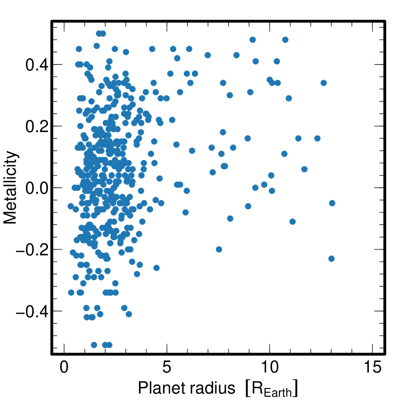
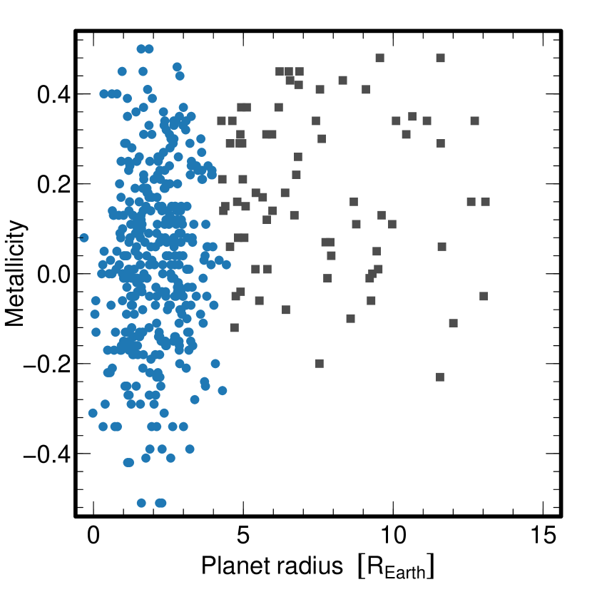
I use the planet host star data from B14. Those data include $T_{\mathrm{eff}},\log{g}$, [M/H], $M_{\ast}$, $R_{\ast}$, and their associated uncertainties. B14 did not include in their planet radius uncertainties the effect of uncertainties in transit depth, even though transit depth uncertainties are more important than the host star radius uncertainties in 25% of the sample. As a result, I supplement the B14 data with the latest Kepler object of interest period and $R_{p}/R_{\ast}$ estimates from the Kepler CasJobs database hosted by the Mikulski Archive for Space Telescopes. I then recompute planet radii from the B14 stellar radii and the updated transit depths. Following B14, I remove from the sample all planets smaller than $3\,R_{\oplus}$ subject to strong stellar irradiation (i.e., $F_{\nu}>5\times 10^{5}$ J s^-1 m^-2), as these planets may have lost a significant fraction of their initial atmospheres. I plot these data in Figure 1.

3. Issues With the Buchhave et al. (2014) Calculation

3.1. An Asymptotically Inconsistent p-value Estimator

An asymptotically inconsistent estimator of a parameter does not converge to the true value of the parameter in the large-sample limit. One problem with the B14 analysis is that they used an asymptotically inconsistent estimator of the $p$-value averaged over planet radius measurement uncertainty in their Monte Carlo simulation. The $p$-value measurements depend on the planet radius measurements, which are subject to measurement uncertainty in the inferred stellar radii $R_{\ast}$ and the measured ratios $R_{p}/R_{\ast}$. The true $p$-values in the absence of uncertainty cannot be measured directly. Instead, one can only measure $p^{\prime}$

$$p^{\prime} = p+N\left(0,\sigma^{2}\right),$$ (1)

where $p$ is the true $p$-value and $N(0,\sigma^{2})$ is due to measurement uncertainties in $R_{\ast}$ and $R_{p}/R_{\ast}$. Repeatedly calculating $p^{\prime}$ after perturbing each planet radius due to the uncertainties in $R_{\ast}$ and $R_{p}/R_{\ast}$ and averaging the result will provide an asymptotically consistent estimate of $p$ by the central limit theorem

$$E\left[p^{\prime}\right] = E\left[p+N(0,\sigma^{2})\right],$$ (2)

$$E\left[p^{\prime}\right] = E\left[p\right]+E\left[N(0,\sigma^{2})\right],$$ (3)

$$\frac{1}{n}\sum_{i=1}^{n}p^{\prime} = \frac{1}{n}\sum_{i=1}^{n}p+\frac{1}{n}\sum_{i=1}^{n}N(0,\sigma^{2}),$$ (4)

$$\overline{p^{\prime}} = \overline{p}+0\Rightarrow\overline{p^{\prime}}=\overline{p}.$$ (5)

B14 never averaged the $p$-value produced for each split point over all iterations. Instead, after each iteration of their Monte Carlo simulation they identified the local $p$-value minima and saved them. After completing 10⁶ Monte Carlo iterations, they determined the mean radii at which local $p$-value minima occurred by averaging over the individual radii calculated on each iteration. In other words, they applied the nonlinear function $f$ that takes a sequence of $p$-values and identifies the radii of local $p$-value minima before averaging over all iterations to identify the mean radii at which $p$-value minima occur. The central limit theorem does not apply in this case, as

$$f(p^{\prime}) = f\left(p+N(0,\sigma^{2})\right),$$ (6)

$$E\left[f(p^{\prime})\right] = E\left[f\left(p+N(0,\sigma^{2})\right)\right],$$ (7)

$$\frac{1}{n}\sum_{i=1}^{n}f(p^{\prime}) = \frac{1}{n}\sum_{i=1}^{n}f\left(p+N(0,\sigma^{2})\right),$$ (8)

$$\overline{f(p^{\prime})} = \overline{f\left(p+N(0,\sigma^{2})\right)}\not\Rightarrow\overline{f(p^{\prime})}=\overline{f(p)}.$$ (9)

As a result, the $p$-values in their Figure 1 improperly account for measurement uncertainty and are asymptotically inconsistent with the true $p$-values absent measurement uncertainty.

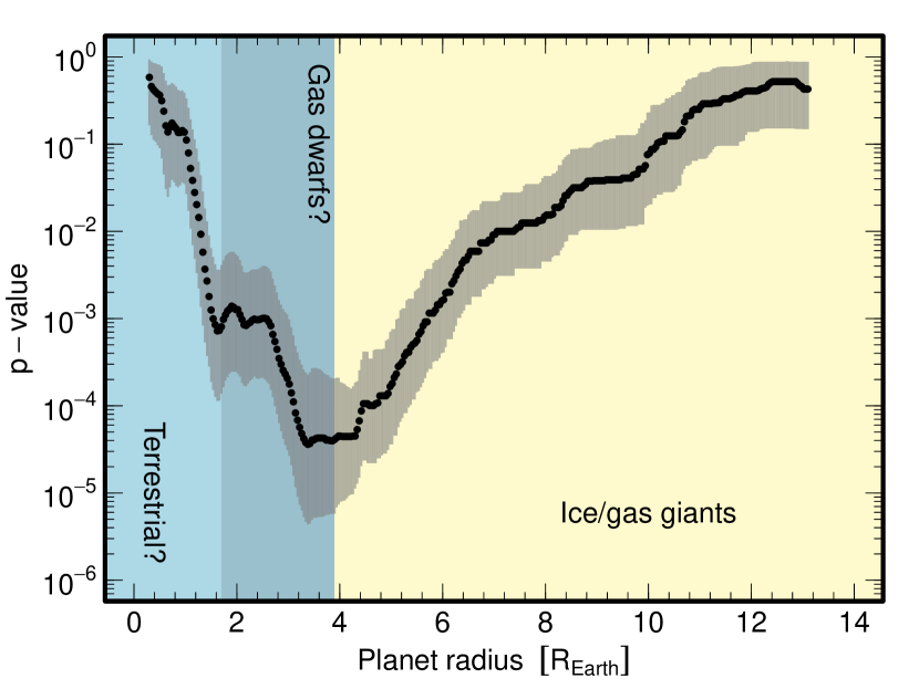
To address that problem, I first generate $10^{5}$ realizations of each planet radius from the distributions that result from the propagation of measurement uncertainties in $R_{\ast}$ and $R_{p}/R_{\ast}$. I split the metallicity data into small-planet and large-planet subsamples at 321 split points from 0.3 to $13.1~{}R_{\oplus}$ in steps of $0.04~{}R_{\oplus}$ and compute the $p$-value from a two-sample Kolmogorov–Smirnov test. I save the resulting $p$-value for each split point and repeat this process $10^{5}$ times. At the end of the calculation, I average the $p$-values for each split point. I plot the result in Figure 2. The apparent local minimum in the $p$-value distribution identified by B14 at $R_{p}=1.7\,R_{\oplus}$ is not present.

3.2. The Multiple Comparisons Problem

Another issue involves the multiple comparisons problem. The multiple comparisons problem occurs in statistical analyses when the same data is both used to select a model and estimate its parameters (e.g., Benjamini, 2010). It frequently leads to the underestimate of the uncertainty of the model parameters. In this case, B14 used the same metallicity data to both identify the planet radius boundaries that separated the three distinct clusters and to estimate the mean metallicity and associated uncertainty for each cluster. Since they used their data both to set the boundaries and determine the mean metallicities for each region, their analysis is subject to the multiple comparisons problem.

One way to correct for this problem is to use independent data sets, one to select the model and another to fit the model parameters. In this case, the correct approach is to split the metallicity data in half. The first half should be used to identify the planet radius boundaries that separate the three distinct clusters of exoplanets. The second half should then be used to infer the average metallicity of each proposed cluster. This process can be repeated a large number of times with different randomly selected subsamples. Consequently, on each iteration of a Monte Carlo simulation, I split the data set described in Section 2 in half. I follow the approach of B14 and identify $p$-value minima at $R_{p}<2\,R_{\oplus}$ and $2\,R_{\oplus}<R_{p}<4\,R_{\oplus}$. I use those planet radii as the boundaries of each exoplanet cluster and use the second half of the metallicity data to compute the mean metallicity of each cluster. I repeat this process $10^{5}$ times. I find that the difference between the mean metallicities for the terrestrial and “gas dwarf” regions is only 0.7$\sigma$—much lower than the 3.1$\sigma$ offset reported by B14.

Metal-poor stars are smaller than metal-rich stars, so a bias toward finding small planets around metal-poor stars in a transit-depth-limited survey is a systematic effect that will further decrease the significance of this offset (Gaidos & Mann, 2013). The fact that the mean metallicities of the stars on either side of the claimed transition at $R_{p}=1.7\,R_{\oplus}$ are indistinguishable contradicts the B14 interpretation of the transition as evidence of different planet formation pathways.

3.3. Do Local p-value Minima Indicate Distinct Exoplanet Regimes?

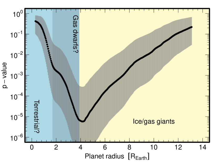
While B14 argue that local minima in a plot of split radius versus $p$-value indicate transitions between distinct exoplanet clusters, this is not always the case. To demonstrate this, I use the same Monte Carlo simulation described in Section 3.1. However, instead of using the observed metallicities, on each iteration I randomly sample the metallicities of stars hosting planets with $R_{p}\leq 1.7\,R_{\oplus}$, $1.7\,R_{\oplus}<R_{p}\leq 3.9\,R_{\oplus}$, and $R_{p}\geq 3.9\,R_{\oplus}$ from their observed distributions. Those distributions are $N(0.00,0.20^{2})$, $N(0.05,0.19^{2})$, and $N(0.18,0.19^{2})$. I plot the result in Figure 3. Despite the fact that distinct metallicity distributions were imposed on each planet cluster, there is no local minimum in the $p$-value distribution at the boundary between the terrestrial and “gas dwarf” planets. The inability of the B14 technique to identify a metallicity boundary imposed by construction as a local $p$-value minimum implies that the technique is not sensitive to subtle features in the metallicity distribution.

4. A More Rigorous Approach

A better way to identify the number of subpopulations required by the planet radius and host star metallicity data is to compare statistical models with varying numbers of components, then identify the model that has the minimum number of parameters yet the maximum likelihood of producing the observed data. I consider two classes of models. First, I fit single-population linear models of the form

$$\mathrm{[M/H]} = a_{0}+\sum_{j=1}^{m}a_{j}R_{p}^{j}+\epsilon,$$ (10)

where $\epsilon$ is the standard uncertainty term in the regression equation. Second, I fit finite Gaussian mixture models with varying numbers of subpopulations of the form

$$\prod_{i=1}^{n}\sum_{j=1}^{m}w_{j}N_{j}(\mathbf{x}_{i}|\mathbf{\mu}_{j},\mathbf{\Sigma}_{j}),$$ (11)

where $\mathbf{x}$ is the data, $m$ is the number of components in the model, the $w_{j}$ are weights such that $\sum_{j=1}^{m}w_{j}=1$, and each $N_{j}$ is a two-dimensional Gaussian component of the overall density

$$N_{j}(\mathbf{x}|\mathbf{\mu}_{j},\mathbf{\Sigma}_{j}) = \frac{1}{2\pi|\mathbf{\Sigma}_{j}|^{1/2}}\times$$ (12)

$$\exp{\left\{-\frac{1}{2}(\mathbf{x}_{i}-\mathbf{\mu}_{j})^{T}\mathbf{\Sigma}_{j}^{-1}(\mathbf{x}_{i}-\mathbf{\mu}_{j})\right\}}.$$

Here $\mathbf{\mu}_{j}$ and $\mathbf{\Sigma}_{j}$ are the mean and covariance of each of the $m$ components of the model. I fit the Gaussian mixture models using the mclust package in R (Fraley & Raftery, 2002; Fraley et al., 2012; R Core Team, 2014).

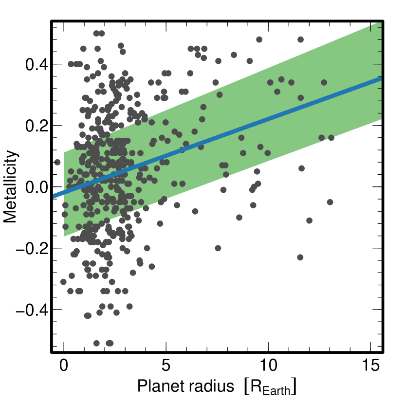
To account for the observational uncertainties, I use a Monte Carlo simulation. I sample the planet radii from the distributions that result from the propagation of measurement uncertainties in $R_{\ast}$ and $R_{p}/R_{\ast}$ and directly use the measured metallicities (since the uncertainty in [M/H] is already reflected in the uncertainty in $R_{\ast}$). On each iteration, I fit linear models of the form of Equation (10) for $m=1,2,\ldots,5$ and Gaussian mixture models $m=1,2,\ldots,7$. I choose both the best linear and Gaussian mixture models using the Bayesian information criterion (BIC; Schwarz, 1978), then use the Akaike information criterion (AIC; Akaike, 1974) to choose between the favored linear and Gaussian mixture models. I repeat this process $10^{3}$ times. In all cases, the best linear model is preferred. For the linear model, the $m=1$ model is favored 76.4% of the time, the $m=2$ model is favored 22.3% of the time, while a higher-order model is favored 1.3% of the time. While the Gaussian mixture model is disfavored relative to the linear model, the two-component model is the best of the mixture models: the two-component model is preferred on 92.8% of the iterations, while the three-component model is preferred 7.2% of the time. I plot representative examples of the BIC-selected models from one iteration of my Monte Carlo simulation in Figure 4.

5. Discussion and Conclusion

The performance of a large number of tests on the same data set without correcting the test thresholds, the use of an asymptotically inconsistent estimator of the $p$-value in the presence of measurement uncertainty, the oversight of the multiple comparison problem, or the inability of the B14 technique to identify an imposed metallicity effect as a $p$-value minimum are all sufficient reasons to be skeptical of the claimed transition at $R_{p}=1.7\,R_{\oplus}$. The problems with the B14 analysis technique cannot be mitigated by examining a larger or independent data set—they are inherent in the analysis technique itself. Instead, the analysis in Section 4 shows that a smooth, one-component linear model is a better fit to the data than any multi-component model. If a multi-component model is used, then the two-component model is consistently a better fit than the three-component model. As a result, the planet radius and metallicity data for the Kepler F and G star planet hosts does not support the idea of multiple types of small planets. Instead, a continuum of planet sizes between $1\,R_{\oplus}$ and $4\,R_{\oplus}$ are likely formed independent of the amount of solids present.

While observational evidence suggests that most planets larger than about $2\,R_{\oplus}$ have significant hydrogen atmospheres (e.g., Marcy et al., 2014), Kepler-10c is an exception with a radius of $2.35\,R_{\oplus}$ and a density of 7.1 g cm^-3 (Dumusque et al., 2014). Likewise, smaller planets probably have a wide range of atmospheric properties (e.g., Rogers, 2014; Wolfgang & Lopez, 2014). Moreover, a wide range of densities can be present even in the same system, with Kepler-36 the best example (Carter et al., 2012). For these reasons, near solar metallicity it does not seem likely that the final masses or compositions of small exoplanets are controlled primarily by the amount of solid material present in their parent protoplanetary disks.

Figure 1.— Planet radius $R_{p}$ vs. host star metallicity.

Figure 2.— Mean $p$-value as a function of planet radius. I split the sample into small-planet and large-planet subsamples at 321 split points from $0.3\,R_{\oplus}$ to $13.1\,R_{\oplus}$ in steps of $0.04\,R_{\oplus}$ and compute the $p$-value from a two-sample Kolmogorov–Smirnov tests on the metallicity distributions of both subsamples. I repeat this process 10⁵ times. The black points are mean $p$-values averaged over the uncertainties in host star radius $R_{\ast}$ and transit depth $(R_{p}/R_{\ast})^{2}$. I indicate the uncertainty at each radius as a semi-transparent gray rectangle with height given by the uncertainty in the $p$-value and width $0.02\,R_{\oplus}$. After accounting for the uncertainties in $R_{\ast}$ and $(R_{p}/R_{\ast})^{2}$, the $p$-values do not support the idea of a qualitative difference between planets with radii above or below $1.7\,R_{\oplus}$.

Figure 3.— Mean $p$-value as a function of planet radius in the scenario advocated by B14 for three distinct planet clusters separated at $1.7\,R_{\oplus}$ and $3.9\,R_{\oplus}$ with metallicity distributions $N(0.00,0.20^{2})$, $N(0.05,0.19^{2})$, and $N(0.18,0.19^{2})$. If planet radius boundaries at $1.7\,R_{\oplus}$ and $3.9\,R_{\oplus}$ do separate the exoplanet population into three clusters with unique metallicity distributions, then that difference would manifest itself as a non-continuous first derivative—a “kink”—at $1.7\,R_{\oplus}$. Even though three unique metallicity distribution were imposed by construction in this case, there is no $p$-value minimum at $1.7\,R_{\oplus}$. Consequently, even if there were three distinct clusters of exoplanets, each with a unique metallicity distribution, the analysis described in B14 would not be able to identify them by $p$-value minima.

Figure 4.— Two different models for the relationship between $R_{p}$ and metallicity. Left: a one-component, linear relationship between $R_{p}$ and metallicity. The blue line shows the best-fit model, while the green-shaded region shows the 25% and 75% quantile regression bands computed using the quantreg package (Koenker, 2013). Right: a Gaussian mixture model with two components. Planets plotted as blue circles are assigned to one component, while gray squares are assigned to the other. The divide between the two populations occurs at $R_{p}\approx 4\,R_{\oplus}$. While the two-component Gaussian mixture model is favored over mixture models with one to seven components, the one-component linear model is favored by the Akaike information criterion (AIC) over any of the mixture models. For that reason, a one-component smooth model is currently the best match to the Kepler planet radius and metallicity data for F and G stars presented in B14.

References

- Akaike (1974) Akaike, H. 1974, ITAC, 19, 716
- Benjamini (2010) Benjamini, Y. 2010, Biom. J., 52, 708
- Buchhave et al. (2014) Buchhave, L. A., Bizzarro, M., Latham, D. W., et al. 2014, Natur, 509, 593
- Buchhave et al. (2012) Buchhave, L. A., Latham, D. W., Johansen, A., et al. 2012, Natur, 486, 375
- Carter et al. (2012) Carter, J. A., Agol, E., Chaplin, W. J., et al. 2012, Sci, 337, 556
- Dumusque et al. (2014) Dumusque, X., Bonomo, A. S., Haywood, R. D., et al. 2014, ApJ, 789, 154
- Dunn (1959) Dunn, O. J. 1959, Ann. Math. Statist., 30, 192
- Dunn (1961) Dunn, O. J. 1961, J. Am. Stat. Assoc., 56, 64
- Fischer & Valenti (2005) Fischer, D. A., & Valenti, J. 2005, ApJ, 622, 1102
- Fraley & Raftery (2002) Fraley, C. & Raftery, A. E. 2002, J. Am. Stat. Assoc., 97, 611
- Fraley et al. (2012) Fraley, C., Raftery, A. E., Murphy, T. B., & Scrucca, L. 2012, mclust Version 4 for R: Normal Mixture Modeling for Model-Based Clustering, Classification, and Density Estimation, Technical Report No. 597 (Seattle, WA: Univ. Wash. Dept. of Statistics)
- Gaidos & Mann (2013) Gaidos, E., & Mann, A. W. 2013, ApJ, 762, 41
- Koenker (2013) Koenker, R., quantreg: Quantile Regression. R package version 5.05 (Champaign, IL: Univ. of Illinois)
- Marcy et al. (2014) Marcy, G. W., Isaacson, H., Howard, A. W., et al. 2014, ApJS, 210, 20
- Mayor et al. (2011) Mayor, M., Marmier, M., Lovis, C., et al. 2011, arXiv:1109.2497
- R Core Team (2014) R Core Team 2014, R: A Language and Environment for Statistical Computing (Vienna: R Foundation for Statistical Computing)
- Rogers (2014) Rogers, L. A. 2014, arXiv:1407.4457
- Santos et al. (2004) Santos, N. C., Israelian, G., & Mayor, M. 2004, A&A, 415, 1153
- Schlaufman & Laughlin (2011) Schlaufman, K. C., & Laughlin, G. 2011, ApJ, 738, 177
- Schwarz (1978) Schwarz, G. E. 1978, AnSta, 6, 461
- Sousa et al. (2008) Sousa, S. G., Santos, N. C., Mayor, M., et al. 2008, A&A, 487, 373
- Wolfgang & Lopez (2014) Wolfgang, A., & Lopez, E. 2014, arXiv:1409.2982