A unified framework for modeling and implementation of hybrid systems with synchronous controllers

Abstract

This paper presents a novel approach to including non-instantaneous discrete control transitions in the linear hybrid automaton approach to simulation and verification of hybrid control systems. In this paper we study the control of a continuously evolving analog plant using a controller programmed in a synchronous programming language. We provide extensions to the synchronous subset of the SystemJ programming language for modeling, implementation, and verification of such hybrid systems. We provide a sound rewrite semantics that approximate the evolution of the continuous variables in the discrete domain inspired from the classical supervisory control theory. The resultant discrete time model can be verified using classical model-checking tools. Finally, we show that systems designed using our approach have a higher fidelity than the ones designed using the hybrid automaton approach.

1 Introduction

Modern closed loop control systems consist of a physical process (termed the plant) controlled by a discrete embedded controller. The plant is a continuously evolving (analog) system, which is sampled by an analog to digital converter at specific intervals. These samples are then input into the discrete controller, which makes decisions depending upon the control logic and feeds the resultant outputs back to the plant to control it. The continuous time nature of the plant and the discrete time nature of the controller together form a hybrid system. The Linear Hybrid Automaton [1] is arguably the most popular approach for modeling such hybrid systems. A linear hybrid automaton captures the continuous evolution of the plant model as first order ordinary differential equations (ODEs). In every control mode of the discrete controller, the plant variables evolve according to a set of ODEs, until an invariant condition holds. As soon as the invariant condition is violated, an instantaneous switch is made by the controller to a different control mode. The continuous variables in the plant model can now evolve with a new set of ODEs. Thus, the controller changes the plant behavior through this mode switch.

Control systems are reactive systems [2] that have an ongoing interaction with their respective plant in terms of discrete time steps. At the start of each time step, the inputs from the plant are captured, a reaction function is called to process these inputs, and finally the outputs are emitted back to the plant. Synchronous languages such as Esterel [3], Lustre [4], Signal [5] are used extensively to implement such reactive systems, since synchronous programs can be translated into transition systems in polynomial time even with exponentially large number of states. Furthermore, model-checking of temporal logic specifications [6] can be directly performed on these resultant symbolic transition systems to guarantee functional and real-time properties of the controller. Synchronous languages, operate based on the principle of synchrony hypothesis, which requires that the reaction function takes zero time and the outputs are produced instantaneously.

Given the instantaneous mode switch of the hybrid automaton and the zero delay computation model of the synchronous languages; it should not be surprising then that controllers modeled in hybrid automaton should be implemented with synchronous languages since semantically, the discrete step: mode switch and the reaction function in both models takes zero time. However, in a real system no controller takes zero time. The synchronous language community has addressed this problem by considering the worst case reaction time (WCRT) of a synchronous program [7]. For a synchronous controller; the WCRT, which is akin to the critical path of a program, determines the inter-arrival time of input events. Statically obtaining a tight WCRT for synchronous controllers is a well studied problem [8, 9, 7]. To the best of our knowledge an equivalent approach to incorporating time-delayed mode switches has not been addressed by the hybrid automaton community. Consequently, any results obtained from a system modeled using a hybrid automaton has low fidelity, i.e., does not behave as expected due delays in making control decisions.

In this paper our main contribution is: a powerful language with a precise formal semantics that allows the modeling, verification and implementation of non-trivial synchronous controllers with time-delays within their continuous environment. Our contributions can be refined as follows:

• Automatic, compiler driven, symbolic representation of the hybrid systems designed in the proposed hybrid synchronous language called HySysJ.

• A precise formal and novel natural semantics for compilation of hybrid systems.

• The discrete approximation of hybrid system designed in HySysJ based on discrete linear time invariant systems from classical supervisory control theory [10].

Rest of the paper is arranged as follows: Section 2 gives a detailed description of the current state of the art in hybrid system design, highlighting the deficiencies. Section 3 introduces the preliminaries required to read the rest of the paper. We motivate the problem using an example in Section 4. The basic language definition is provided in Section 5, which is further extended with continuous time constructs and semantics in Section 6. The relation of the proposed approach to classical supervisory control theory is presented in Section 7. The verification procedure carried out on the motivating example in the resultant new language is given in Section 8. Finally, we conclude in Section 9.

2 Related work

Many languages have been proposed for modeling and verification of Hybrid systems. A good survey can be found in [11]. The first class of languages are the hardware description languages enhanced with the analog mixed signal (AMS) extensions, such as; VHDL-AMS and SystemC-AMS [12, 13]. These languages lack any sort of formal semantics and hence, cannot be used for formal verification. The second class is the data-flow languages such as Zélus and SCADE/Lustre [14, 4], which approximate the continuous ODEs. This approach of approximating the continuous ODE behavior is essential, because model-checking most system properties, including safety properties, are known to be undecidable for general hybrid systems [1]. The aforementioned data-flow languages are also endowed with formal mathematical semantics. This conjunction of approximation of continuous behavior along with formal mathematical foundations makes these languages potentially suitable for model-checking. But, unlike us, the overall hybrid model does not account for the non-zero mode-switch times and hence, these programming languages suffer from the same problems as the hybrid automata.

Finally, the work closest to the one described in this article is done by: (1) Closse et al. [15], where they extend the Esterel language to model timed automata [16], i.e., ODEs with rate of change always equal to 1. In this proposal we are able to model the more general hybrid rather than its subset timed automaton and (2) Baldamus et al. [17], which is a seminal work in extending synchronous imperative languages to model hybrid automaton. This work is extended further and completed by giving a formal treatment by Bauer et al. [18]. The work described herein differs significantly from both; [18] and [17] in that they do not approximate the continuous behavior of the plant, instead all discrete transitions are carried out and then a so called continuous phase is launched, which models the continuous evolution of the plant until the invariant condition holds, just like in hybrid automaton. Since these approaches derive their semantics from hybrid automaton, they inherit the same problem described in Section 4, i.e., non-zero mode-switch transitions cannot be captured in the semantics.

Overall, the formal foundations of the modeling/implementation language proposed in this paper are truly unique, since the semantics unify the real-time analysis of synchronous programs [7] and the hybrid modeling languages into a single framework inspired from classical supervisory control theory.

3 Preliminaries

In this section we give the background information required for understanding the rest of the paper.

3.1 The hybrid automaton

We use the definition of linear Hybrid automaton from [1].

Definition 1.

A hybrid automaton H is a tuple $(Loc,Var,Con,Lab,Edge,Act,Inv,Init)$ where

• $(Loc,Var,Con,Lab,Edge,Act,Inv,Init)$ is a labelled transition system with $Loc$ a finite set of locations, real-valued variables $Var$, $V$ the set of valuation $v:Var\rightarrow\mathbb{R}$, and $\Sigma=Loc\times V$ the set of states, $Init\subseteq\Sigma$ of initial states.

• A function $Con:Loc\rightarrow 2^{Var}$ assigning a set of controlled variables to each location

• a finite set of labels $Lab$, including the stutter label $\tau\in Lab$.

• $Act$ (Activities) is a function assigning a set of activities $f:\mathbb{R}_{\geq 0}\rightarrow V$ to each location ($l\in Loc$) which are time-invariant meaning that $f\in Act(l)$ implies $(f+t)\in Act(l)$ where $(f+t)(t^{\prime})=f(t+t^{\prime}),\forall t^{\prime}\in\mathbb{R}_{\geq 0}$

• a function $Inv$ assigning an invariant $Inv(l)\subseteq V$ to each location $l\in Loc$.

• A finite set $Edge\subseteq Loc\times Lab\times 2^{V^{2}}\times Loc$ of edges including $\tau$-transitions $(l,\tau,Id,l)$ for each location $l\in Loc$ with $Id=\{(v,v^{\prime})|\forall x\in Con(l).v^{\prime}(x)=v(x)\}$, and where all edges with label $\tau$ are $\tau$-transitions.

Definition 2.

The semantics of a hybrid automaton $H$ is given by the operational semantics consisting of two rules, one for discrete instantaneous transition steps and one for continuous time steps.

• Discrete step semantics (mode-switch semantics):

  $$\frac{(l,a,(v,v^{\prime}),l^{\prime})\in Edge\ \ v^{\prime}\in Inv(l^{\prime})}{(l,v)\xrightarrow{a}(l^{\prime},v^{\prime})}$$

• Time step semantics

  $$\frac{f\in Act(l)\ f(0)=v\ f(t)=v^{\prime}\ t\geq 0\ f([0,t])\subseteq Inv(l))}{(l,v)\xrightarrow{t}(l^{\prime},v^{\prime})}$$

An execution step $\rightarrow=\xrightarrow{a}\cup\xrightarrow{t}$ of H is either a discrete step or a time step. A path $\pi$ of H is a sequence $\sigma_{0}\rightarrow\sigma_{1}\ldots$ with $\sigma_{0}=(l_{0},v_{0})\in Init$, $v_{0}\in Inv(l_{0})$, and $\sigma_{0}\rightarrow\sigma_{i+1}\forall i\geq 0$.

3.1.1 An example linear hybrid automaton

We will use a closed loop manufacturing system example shown in Figure 1 to elaborate the semantics of hybrid automata.

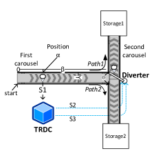
Figure 1: The pictorial representation of the manufacturing control system

(a) The hybrid automaton modelling the manufacturing control system

(b) The behavior of the manufacturing control system as modeled by the hybrid automaton

Figure 2: A simple carousel control system and its hybrid automaton

Consider that we are designing an automated ice-cream manufacturing system as shown in Figure 1. The system consists of two carousel belts that carry an ice-cream to either Storage1 or Storage2 depending upon the RFID tag on the ice-cream. The size of the first carousel is $\beta\times\gamma$ units. A diverter is placed at the end of the first carousel, $\beta$ units from the start. A tag reader and diverter controller (TRDC) is placed at position $\alpha$ from the start of the first carousel. When the ice-cream is detected, the TRDC reads the tag on the ice-cream and then sends a control message to the diverter in order to move it into the correct position, so that once the ice-cream reaches position $\beta$, it is diverted to the correct storage station. The detection of the ice-cream on the first carousel is indicated by the emission of signal $S1$. Signal $S2$, emitted from the TRDC, moves the diverter $\theta$ arc-length units in order to divert the ice-cream to Storage1, while signal $S3$ does the opposite. Furthermore, the carousel and the diverter move at a constant velocity of 1.

The hybrid automaton modeling the manufacturing system is shown in Figure 2a. The elements of the tuple defining the syntax of the hybrid automaton are indicated in Figure 2a for sake of understanding. Initially, the ice-cream and the diverter are at position 0, denoted by the continuous variables $x$ and $y$, respectively. In mode A, the ice-cream travels on the first carousel at a constant velocity of 1 until it reaches position $\alpha$. As soon as the ice-cream reaches $\alpha$, signal $S1$ is emitted with the TAG value Storage1, say. Signal $S2$ is emitted instantaneously and the hybrid automaton moves to mode B. In this mode, the ice-cream and the diverter, both move at a constant velocity until the diverter covers the distance of $\theta$ arc-length units. Finally, a transition is made to mode D, where any further distance until $\beta$ is covered by the ice-cream and then the ice-cream moves onto the second carousel and is placed into the correct storage.

The movement of the ice-cream for this hybrid automaton assuming $\alpha=3$, $\beta=10$ and $\theta=6$ is shown in Figure 2a. Assuming instantaneous discrete mode-switch model of the hybrid automaton, choosing $\alpha=3$ is a feasible solution as seen in Figure 2a. The ice-cream is detected at position 3 on the first carousel and an instantaneous move is made to control mode B where the ice-cream moves another 6 units ending up at position 9 when the hybrid automaton is in mode D, which is less than $\beta=10$.

3.2 The synchronous controller

Definition 3.

A synchronous controller is a tuple $(Q,q_{0},I,O,A,T)$ where:

• $Q$ is the set of states

• $q_{0}\in Q$ is the starting state

• $I$ is the set of input signals

• $O$ is the set of output signals

• $A$ is the set of actions

• $T$ is the transition relation: $T\subseteq Q\times\mathcal{B}(I)\times 2^{A}\times 2^{O}\times Q$. $\mathcal{B}(I)$ is a Boolean expression over the symbols in $I$.

Simply put, a synchronous controller is a directed graph with edges carrying the labels of the form $b/A^{\prime},O^{\prime}:b\in\mathcal{B}(I),A^{\prime}\subseteq A,O^{\prime}\subseteq O$. Intuitively, each edge can be taken if the Boolean condition on the edge holds true. Furthermore, actions (functions) are performed and output signals emitted upon taking the transition.

3.2.1 The timing semantics of synchronous controllers

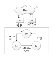
(a) Synchronous controller controlling a plant

(b) Synchronous controller timing diagram

Figure 3: An example synchronous controller and its timing diagram

Figure 3a shows a simple example of a synchronous controller controlling a plant. The controller’s input signal set is $\{I1,I2\}$ and output signals are produced from the set $\{O1,O2\}$. The transition system for the controller is also shown in Figure 3a. There are three states in the transition system. The initial state is labeled S0. When signal $I1$ is produced from the plant, the controller makes a transition to state S1. In the process also emitting signal $O1$ back to the plant. Next, when signal $I2$ is produced from the plant, the controller makes a transition to state S2. Furthermore, the controller performs an action $F$ and outputs signal $O2$ back to the plant.

The timing diagram for the controller is shown in Figure 3b. Every synchronous controller, following the zero delay model [3], progresses in lockstep with a logical clock tick. The inputs are captured from the plant at the start of the logical tick, a reaction function is called to process these inputs (in this case the reaction function is the transition system in Figure 3a) and finally the outputs are produced at the end of the tick. The logical ticks are shown as bars in Figure 3b. At logical tick 1, the input signal $I1$ is captured from the plant, and the output signal $O1$ is instantaneously produced at the end of the logical tick. Similarly, input signal $I2$ is captured at the start of tick 4 and output signal is emitted back to the plant at the end this tick – instantaneously.

Unfortunately, execution of every reaction to the input signals takes some $\delta$ physical time. The zero delay model implicitly requires that the reaction to the input signals be fast enough in order to not miss any input events from the plant. In order to satisfy this implicit restriction, we need to calculate the Worst Case Reaction Time (WCRT) from amongst all the reaction times, which needs to be shorter than the inter-arrival between any two incoming events. Formally, let $\{\delta_{1},\ldots,\delta_{N}\}$ be the set of all possible reaction times for some synchronous controller. Then, $\exists i\in N$, where $WCRT=max(\delta_{i})$. WCRT of any synchronous controller can be calculated statically irrespective of the plant model. Many different techniques exist for the calculation of the WCRT of a synchronous controller [9].

4 The problem of time-delayed mode switches

Let us revisit the manufacturing control system example in Section 3.1.1 and use a synchronous language to implement the TRDC controller that performs the discrete mode switches in Figure 2a. Since the length ($\beta$), the width ($\theta$) of the first carousel and the speed of movement of the carousel and the diverter are all fixed, we only need to place the TRDC at the correct position on the first carousel so that the diverter is in the correct position by the time ice-cream reaches position $\beta$. Our goal is to statically verify that any ice-cream on the first carousel will be diverted to the correct storage depending upon its tag. A hybrid automaton should help us model this system to guarantee this safety property. Note that the reader should interpret the term verify loosely, because the reachability problem for hybrid automata are known undecidable [19].

4.1 The hybrid automaton and the worst case reaction time of synchronous controllers

(a) Difference between the modeled system and the real system.

(b) Missed item tag due to WCRT

Figure 4: The different movement of the ice-cream – hybrid automaton model vs. the real system

The movement of the ice-cream in the real system with the TRDC placed at position 3 (as obtained from the hybrid automaton model) is shown in Figure 4a, bottom graph. Every decision made by the controller does take some time. In case of synchronous controllers, this time is the WCRT. Suppose that $WCRT=2$ units for the TRDC controller, then the ice-cream is at position 5 when the hybrid automaton moves to mode B. Now, the system modeled by the hybrid automaton and the real implementation are not in-sync. In fact, when the system enters mode D, the invariant $x\leq\beta$ does not hold and the transition is immediately made back to mode A. But, the ice-cream is already at position 11 when the system enters mode D, which is past $\beta=10$ and hence, the ice-cream now moves to Storage2 rather than Storage1 as desired, thereby violating the safety property. Overall, the model does not reflect reality and needs to be modified. One might assume that the transition time of the controller is orders of magnitude smaller compared to the speed of movement of the ice-cream on the carousel and hence, can be considered as zero. This is a very rough approximation as indicated in [20]. There are data acquisition delays, sensor delays, communication delays, computation delays in digital controllers, which cannot be ignored with the slight of hand. These delays need to be accounted for in the WCRT of the embedded controller.

4.2 The hybrid automaton, the worst case reaction time and the synchrony hypothesis

Every synchronous program can be statically analyzed to find its WCRT. As mentioned before (see Section 3.2) the synchrony hypothesis is guaranteed iff the inter-arrival time of input events is less than or equal to $WCRT$. For the manufacturing system example $WCRT=2$, hence, the synchronous control logic (TRDC), in the worst case, samples inputs every 2 units of time. An input is generated when the ice cream reaches position 3 (since $\alpha=3$), but under the synchrony assumption, this input is missed as this input event is not aligned with the edge of the controller clock, i.e., it is not divisible by $WCRT=2$ (see Figure 4b). An event driven system would, on the other hand, easily capture this input event. Hence, there is an implicit assumption in the hybrid automaton that the control logic is event driven rather than clock-driven as is the case with synchronous controllers. This is yet another problem that needs to be addressed when designing synchronous controllers.

The aforementioned problems occur due to the non-zero reaction time of the synchronous controllers. More precisely, the plant makes progress while the controller carries out internal computations, unlike in the hybrid automaton where these discrete mode-switches zero time. This plant behavior could be modeled by labeling the discrete transitions in the hybrid automaton with differential equations. But, this solution does not bode well with the semantics of the hybrid automaton. The time for the discrete transition depends upon the implementation of the controller, which differs depending upon the underlying platform, compiler technology, etc. Hence, if we were to simply label the discrete transitions with differential equations, the evolution of the continuous plant variables would depend upon the speed of the controller, which is in stark contrast to the semantics of the hybrid automaton [1]. In light of these problems we need a new programming model for design and verification of hybrid systems. In the rest of the paper we present a power language called HySysJ that: (1) results in high fidelity hybrid system models, by incorporating time-delayed mode switching, (2) allows automatically extracting controllers for implementation from the hybrid model and (3) allows for automatic formal verification of the hybrid system.

5 The base language

The proposed language HySysJ builds atop the synchronous subset of the SystemJ [21] programming language, which is itself inspired from Esterel [3]. The core kernel statements of the language are given in Figure 5.

$$\begin{array}[]{ll}stmt&::=stmt_{0}[\mathrm{``||"}stmt]\\ stmt_{0}&::=stmt_{1}[``;"stmt_{0}]\\ stmt_{1}&::=\\ &|``\mathbf{nothing}"|``\mathbf{emit}"\ a|``?"a``="expr\\ &|``\mathbf{pause}"|``\mathbf{abort}"``("[``\mathbf{immediate}"]expr``)"stmt\\ &|``\mathbf{if}"``("expr``)"stmt``\mathbf{else}"stmt\\ &|``\mathbf{suspend}"``("[``\mathbf{immediate}"]expr``)"stmt\\ &|[``\mathbf{input}"|``\mathbf{output}"][type]``\mathbf{signal}"a\ [op\ ``="expr]\\ &|``\mathbf{loop}"stmt|``\{"stmt``\}"\\ op&::=``\mathbf{op+}"|``\mathbf{op*}"\end{array}$$

Figure 5: The core kernel statements of the synchronous subset of SystemJ. The terminals appear within double quotes, and angular brackets indicate optional syntactic components.

The core synchronous language constructs in SystemJ are borrowed directly from Esterel. The $\mathbf{nothing}$ construct terminates instantaneously and is primarily used in the structural operational semantics during term rewriting. Every signal is declared via the $\mathbf{signal}$ declaration statement. The $type$ declaration for a signal is optional. A non-typed signal is considered to be a pure signal whose status can be set to $true$ for one logical tick by emitting it (via $\mathbf{emit}$) and is $false$ if it is not emitted in that logical tick. A valued signal has a value and a status. Every valued signal is uniquely associated with one of the types: $\mathbf{ratio}$, $\mathbf{integer}$, or $\mathbf{boolean}$. A signal can be emitted multiple times with different values in the same logical tick. In such cases, signal values are combined with operators defined during signal declaration. Only associative and commutative operators (e.g., $\mathbf{op+}$ and $\mathbf{op*}$) are permitted over signal values and everything must be well-typed in the expected way. Unlike the status of a signal, the value of a signal is persistent over logical ticks. A block of statements can be preempted or suspended for a single tick using $\mathbf{abort}$ and $\mathbf{suspend}$ constructs, respectively. The $\mathbf{if}$ construct is the usual branching construct, operating on the status or values of signals. Moreover, one or more of the aforementioned statements can be run in lockstep parallel using the synchronous parallel operator $||$. Finally, the $\mathbf{loop}$ construct is used to write temporal loops, whereby each iteration consumes a logical tick via the $\mathbf{pause}$ construct.

The synchronous semantics of SystemJ differs from Esterel in one significant way: the emission of every signal is delayed by a single logical tick and is only visible in the next iteration of the synchronous program. We describe these so called delayed signal semantics using simple code snippets shown in Figure 6.

⬇ 1 signal S, A, B; 2 emit S; 3 if (S) emit A else emit B; 4 pause

(a) Synchronous program code snippet 1

(b) SystemJ logical timing behavior

⬇ 1 signal S, A, B; 2 emit S; 3 pause; //additional pause 4 if (S) emit A else emit B; 5 pause

(c) Synchronous program code snippet 2

(d) SystemJ logical timing behavior

Figure 6: SystemJ vs. Esterel logical timing behavior

Figure 6a shows a very simple synchronous program. Three pure signals S, A, and B are declared. Signal S is emitted and then its status is checked for presence, if this signal has been emitted, then signal A is emitted, else signal B is emitted. Finally, the program ends with the $\mathbf{pause}$ statement indicating the end of the logical tick. The logical timing behavior of this SystemJ program is shown in Figure 6b. In SystemJ, the emission of signal makes its visible only in the next logical tick, hence, this program emits signal B in the first logical tick. The logical timing behavior achieved by slightly changing the program (inserting an additional $\mathbf{pause}$ construct) is shown in Figures 6c and 6d. In this case, since signal S is emitted in tick-1, its status is true in tick-2 and hence, SystemJ following the so called delayed signal semantics emits signal A in the second tick.

Valued signals follow rules similar to signal statuses, i.e., reading a value of the signal (e.g., $?S$) always gives the value from the previous logical tick or the default value (0 usually), while setting the value of the signal (e.g., $?S=2$) always sets the current value. The previous value of the signal is updated to the current value at the end of the logical tick.

⬇ 1 ?S = ?S + 1

Figure 7: Code snippet – incorrect in Esterel, but correct in SystemJ

This so called delayed signal semantics implicitly avoid plethora of problems that plague Esterel programs, related to causality. Consider the code snippet in Figure 7. In case of Esterel, the value of signal S is fed back to itself in the same logical tick, and hence, in Esterel, one needs to check that ?S == (?S + 1), which obviously has no solution. But, in SystemJ, since the signal values are only ever updated at the end of a logical tick, the program in Figure 7 is computable.

Now that we have described the base language and its syntactic constructs, we are ready to introduce the continuous elements into the synchronous subset of SystemJ that will result in the new HySysJ hybrid system specification language.

6 HysysJ – introducing continuous time in synchronous SystemJ

The most fundamental modification to the synchronous language described in Section 5 is the introduction of continuous variables and related actions that manipulate these variables. Following standard practice, we will first introduce the syntactic extensions and then describe the semantics.

$stmt_{1}$	$::=stmt_{2}$
$stmt_{2}$	$::=$
	$|``\mathbf{cont}"a\ [op\ ``="\ expr]$
	$|``\mathbf{cont}"a\ [``="\ expr]$
	$|\ a=expr$
	$|``\mathbf{do}``\{"stmt_{3}``\}"``\mathbf{until}"``("expr``)"$
$stmt_{3}$	$::=$
	$|\ a``^{\prime}"=expr$
	$|\ a``^{\prime}"=expr[``||"stmt_{3}]$

(a) The syntactic constructs for continuous variable declaration and manipulation

⬇ 1 signal R; 2 abort (R) 3 loop { 4 a = a + $\rho$ * WCRT; 5 if (!TTL ($[a^{\prime}=\rho]$, $expr$, $\{a\}$)) emit R; 6 pause 7 }

(b) The rewrite for the derived construct: $\mathbf{do}\ \{a^{\prime}=\rho\}\mathbf{until}(expr)\}$.

⬇ 1 signal R; 2 abort (R) 3 loop { 4 a = a + $\rho$ * WCRT; b = b + $\sigma$ * WCRT; 5 if (!TTL ($[a^{\prime}=\rho,b^{\prime}=\sigma]$, $expr$, $\{a,b\}$)) emit R; 6 pause 7 }

(c) The rewrite for the derived construct: $\mathbf{do}\ \{a^{\prime}=\rho||b^{\prime}=\sigma\}\mathbf{until}(expr)\}$.

Figure 8: The continuous variables and derived construct operating on these variables in HySysJ

6.1 Syntax of continuous actions

The syntactic extensions to declare and manipulate the continuous variables are given in Figure 8a. Every continuous variable is declared with the qualifier $\mathbf{cont}$. A default value can be specified during declaration. Uninitialized continuous variables take a default value of 0. Furthermore, a commutative and associative operator ($op$) can be used to combine the values of the continuous variables, just like in case of valued signals. The type of every continuous variable is a $\mathbf{ratio}$.

Two forms of syntactic extensions are allowed for manipulating continuous variables: (1) a direct assignment to the continuous variable or use of continuous variables in expressions, called instantaneous actions and (2) writing first order ODEs inside a $\mathbf{do}\ \mathbf{until}\ (expr)$ block that evolve the continuous variables, called flow actions. We use primed symbols (e.g., a^′ = c, where c is some constant) to describe these first order derivatives. One or more such ODEs can be specified inside the $\mathbf{do}$ block. The synchronous parallel operator $||$ is used to specify more than one ODE inside the $\mathbf{do}$ block. Every ODE inside the $\mathbf{do}$ block is evaluated simultaneously until the $expr$ (the so called invariant condition) holds true. The $\mathbf{until}$ $expr$ is required to evaluate to a Boolean $true$ or $false$ value.

6.2 Semantics of continuous actions

6.2.1 Instantaneous actions

Instantaneous actions are so called, because the statement terminates instantaneously without consuming a logical tick. Examples of instantaneous actions are shown in Figure 9. These include; assigning a value to a continuous variable, reading the value of a continuous variable, assigning the value of the continuous variable to a valued signal or another continuous variable, etc.

Continuous variables, like signals, follow delayed semantics. Hence, using a continuous variable in an expression (right hand side in case of an assignment statement) always gives the value from the previous logical tick or the default value. A new value is assigned to a continuous variable only at the end of the current logical tick.

In Figure 10a, continuous variable a is first declared, with a default value of 0, and then assigned a value of 1. Next, an if else block is used to check the value of a. If the value of a is 1, then signal S1 is emitted else signal S2 is emitted. The same program is presented in Figure 10b, except that a pause statement is inserted after the assignment statement: a = 1. In the first case, due to delayed semantics, when the value of a is read in the if expression, the return value is 0 (the default value) and hence, signal S2 is emitted. On the other hand, in Figure 10b when the program flow reaches the if statement, it is the second logical tick and hence, the value of a is 1 (assigned in the previous logical tick) thus signal S1 is emitted.

It is important to note that the name instantaneous action does not mean that the value of the continuous variable changes instantaneously. Every continuous variable changes its value only at the end of the tick. The name instantaneous action only implies that the statement itself is instantaneous and does not consume logical ticks.

⬇ 1 cont a = 0; //declaring a continuous variable with initial value 0 2 a = 1; // assigning value 1 to continuous variable a 3 if (a == 1) emit S; //continuous variable used in expression. 4 ?S = a; //value of continuous variable a assigned to a valued signal.

Figure 9: Instantaneous actions on continuous variables in HySysJ

⬇ 1 signal S1, S2; //declaring pure signals 2 cont a; //declaring a with default value 0 3 a = 1; // assigning value 1 to continuous variable a 4 if (a == 1) emit S1 //continuous variable used in expression. 5 else emit S2; 6 pause

(a) Code snippet 1

⬇ 1 signal S1, S2; //declaring pure signals 2 cont a; //declaring a with default value 0 3 a = 1; // assigning value 1 to continuous variable a 4 pause; 5 if (a == 1) emit S1 //continuous variable used in expression. 6 else emit S2; 7 pause

(b) Code snippet 2

Figure 10: Instantaneous actions on continuous variables in HySysJ with delayed semantics

6.2.2 Flow actions

The flow actions are programmed using $\mathbf{do}$ $\mathbf{until}$ blocks and are first order ODEs with a constant rate of change. In the example in Figure 11a, continuous variable a is declared and initialized to a value of 0, which is an instantaneous action. Next, this variable evolves continuously until its value is 2 inside a $\mathbf{do}$ $\mathbf{until}$ block. In the next example, two variables; a and b evolve together until the invariant condition ($\mathbf{until}$ expression) holds. One can also combine multiple such flow actions together in synchronous parallel (Figure 11d). Finally, HySysJ also allows preempting flow actions using the standard preemptive constructs from the base language.

⬇ 1 cont a = 0; 2 do {a^′ = 1} until (a <= 2)

(a) Example with one continuous variable

⬇ 1 cont a = 0, b = 0; 2 do {a^′ = 2 || b^′ = 2} until (a <= 16 && b <= 10)

(b) Example with two continuous variables

⬇ 1 cont a = 0, b = 0; 2 do {a^′ = 1 || b^′ = 1} until (a <= 10 && b <= 6)

(c) Another example of two continuous variables

⬇ 1 cont a = 0, b = 0; 2 do {a^′ = 1} until (a <= 10) || do {b^′ = 1} until (b <= 6)

(d) Example of parallel composition of flow actions

⬇ 1 signal S; 2 cont a = 0; 3 abort(S) { do {a^′ = 1} until (true) } || {pause; emit S; pause}

(e) Example of preemption of continuous variable evolution

Figure 11: Examples of continuous actions in HySysJ

Semantics and intuitive explanation for simple flow actions

In this section we describe the rewrite semantics of simple flow actions and give the intuitive explanation for these rewrites. A complete formal treatment is provided in Appendix A.

Consider the simple flow action in Figure 11a; variable a evolves linearly with time until it reaches the value 2. The first order ODE in Figure 11a has the solution: $a=\int 1\times\mathrm{d}t=1\times t+C$, where 1 is the rate of change of a and $C$ is the initial value of a. Furthermore, the $\mathbf{until}$ expression gives the upper bound on this indefinite integral. For this very simple flow action, the upper bound of the indefinite integral is 2. Hence, the value of a is: $a=[t]^{2}_{0}+C=2+C$. From Figure 11a, we also know that the initial value of a is 0, i.e., $C=0,\therefore a=2$.

$$\int_{0}^{k}\rho\times\mathrm{d}t+C=\sum_{n=0}^{k-1}\ \rho\times\Delta t+a[0]$$ (1)

$$\therefore a[k]=a[0]+\sum_{n=0}^{k-1}\ \rho\times WCRT$$ (2)

The main idea of our rewrite is to approximate the continuous evolution of a using a discrete time model. Equation (1) gives this approximation. We take advantage of the synchronous nature of our programming language. Every HySysJ program proceeds in discrete logical ticks, the value of variable a at tick 0 (the initial value) is denoted $a[0]$. Similarly, for some tick $n$, the value is denoted by $a[n]$. In Equation (1), $\Delta t$ is the time between two discrete logical ticks, which is the WCRT as stated in Section 3.2 and can be computed statically for any HySysJ program [9]. $\rho$ is the rate of change, which is always a constant for any linear ODE. Finally, the upper bound of the summation ($k-1$) is dependent upon the $\mathbf{until}$ expression.

Equation (2) obtained from Equation (1) is clearly a bounded reduction on a (using sum), which in any imperative language is written using a bounded loop. Hence, our rewrite for any linear ODE is a bounded temporal loop computing the value of the continuous variable as shown in Figure 8b. In Figure 8b the temporal loop performing reduction on a spans from lines 3 to 7. The actual reduction is performed on line 4. This temporal loop is exited using a combination of $\mathbf{emit}$ and $\mathbf{abort}$ constructs as shown on lines 2 and 5. Finally, the upper bound $k$ is Equation (2) is computed dynamically in the rewrite using procedure TTL (Time To Live) shown in Algorithm 1. In the general case it is impossible to statically (at compile time) compute the upper bound $k$ in Equation (2), since one can have complex invariant conditions specified in the $until$ expressions and hence, dynamically (at program execution time) deciding when to abort the temporal loop is the only viable option.

Delayed semantics play a crucial role in the rewrite of Figure 8b.

• Computability of the reduction: Reading the value of a (line 5) always gives the value from the previous tick. Writing to a succeeds only at the end of the logical tick, i.e., when the control flow reaches the $\mathbf{pause}$ construct on line 6. The delayed semantics make the reduction computable. Moreover, the updated value of a is stable and observable only at the end of the tick following delayed semantics.

• The TTL algorithm: The TTL algorithm, which decides when to abort the infinitely running temporal loop is also dependent upon the delayed semantics. The $\mathbf{abort}$ construct (line 2) checks if the status of signal R is set to true in the previous logical tick (statuses of signals are false upon declaration), following delayed semantics, and if so, aborts the loop performing the reduction. Signal R is emitted inside the loop body (line 5), provided the Boolean value returned from the TTL algorithm in not true. The status of R is updated only at the end of the tick (line 6, which is also completion of iteration of the loop). Hence, we are guaranteed that at least one iteration of the temporal loop will take place, irrespective of the invariant in the $\mathbf{until}$ expression.

  From Equation (2), we know that $a[k]$ for some tick $k$ satisfies the $\mathbf{until}$ invariant. Obviously, $a[k-1]$ should also satisfy this invariant condition. But, $a[k+1]$ should never satisfy the $\mathbf{until}$ invariant. Due to delayed semantics, we now know that given $a[k-1]$, $a[k]$ will always be computed. In order not to reach tick $k+1$ (since $a[k+1]$ violates the $\mathbf{until}$ invariant) signal R should have its status set to true at the end of tick $k$. Hence, the signal R (line 5) should be emitted in the program transition from tick $k-1$ to $k$ (denoted as $[k-1,k)$). But, during this program transition, we only know the value $a[k-1]$, which consequently means that algorithm TTL needs to look ahead 2 ticks ($k+1-(k-1)=2$) and return a Boolean value true if it satisfies the $\mathbf{until}$ invariant and false otherwise. If invariant condition is satisfied 2 ticks from now, then one more iteration of the loop is allowed to be carried out, else the loop terminates at the end of the current program transition.

Input : $\Omega$: a list of ODEs from one $\mathbf{do}$ block

Input : $expr$: the $\mathbf{until}$ expression

Input : $\mathcal{V}$: the set of continuous variables in $\Omega$

Result: a Boolean value

1 $\Delta$ $\leftarrow$ $\emptyset$;

2 for each $v$ in $\mathcal{V}$ do

3       $\tau$ $\leftarrow$ $[\![v]\!]$ + $2$ * get_rho (filter ($\Omega$, $v$)) * WCRT ;

       // Union the value $\tau$ of $v$ two ticks from now in set $\Delta$

4       $\Delta$ $\leftarrow$ $\Delta\cup\{v\rightarrow\tau\}$;

5      

6end return holds_at_delta ($expr$, $\Delta$);

ALGORITHM 1 Algorithm to calculate TTL

⬇ 1 cont a = 0; 2 signal R; 3 abort (R) 4 loop { 5 a = a + WCRT; 6 if (!TTL ([$a^{\prime}=1$], a<=2, $\{a\}$)) 7 emit R; 8 pause 9 }

(a) Rewrite for flow action in Figure 11a

(b) The timing diagram for Figure 12a

⬇ 1 cont a = 0, b = 0; 2 signal R; 3 abort (R) 4 loop { 5 a = a + (2 * WCRT); 6 b = b + (2 * WCRT); 7 if (!TTL ([$a^{\prime}=2$, $b^{\prime}=2$], 8 a<=16 && b<=10, $\{a,b\}$)) 9 emit R; 10 pause 11 }

(c) Rewrite for flow action in Figure 11b

(d) The timing diagram for Figure 12b

Figure 12: Rewrites for the flow actions in Figure 11 with WCRT = 2

⬇ 1 cont a = 0, b = 0; 2 signal R; 3 abort (R) 4 loop { 5 b = b + WCRT; 6 a = a + WCRT; 7 if (!TTL ([$a^{\prime}=1$, $b^{\prime}=1$], 8 a<=10 && b<=6, $\{a,b\}$)) 9 emit R; 10 pause 11 }

(e) Rewrite for flow action in Figure 11c

(f) The timing diagram for Figure 12e

⬇ 1 cont a = 0, b = 0; 2 { 3 signal R; 4 abort (R) 5 loop { 6 a = a + WCRT; 7 if (!TTL ([$a^{\prime}=1$], 8 a<=10, $\{a\}$)) 9 emit R; 10 pause; 11 } 12 } || { 13 signal R; 14 abort (R) 15 loop { 16 b = b + WCRT; 17 if (!TTL ([$b^{\prime}=1$], 18 b<=6, $\{b\}$)) 19 emit R; 20 pause; 21 } 22 }

(g) Rewrite for flow action in Figure 11d

(h) The timing diagram for Figure 12g

Figure 12: Rewrites for the flow actions in Figure 11 with WCRT = 2

⬇ 1 signal S; 2 cont a = 0; 3 abort (S) { 4 loop { 5 a = a+WCRT; 6 loop pause 7 } 8 }||{pause; emit S; pause}

(i) Rewrite for flow action in Figure 11e

(j) The timing diagram for Figure 12i

Figure 12: Rewrites for the flow actions in Figure 11 with WCRT = 2

We use the example in Figure 11a and its rewrite in Figure 12a to explain how the required TTL algorithm behavior is achieved. In the rest of the paper we assume for sake of understanding that the statically computed WCRT value of every HySysJ program is 2 units. The TTL algorithm (Algorithm 1) takes 3 inputs: (1) a list of ODEs ($\Omega$) within one $\mathbf{do}$ block, (2) the $\mathbf{until}$ invariant ($expr$), and (3) the set of continuous variables evolving in the $\mathbf{do}$ block ($\mathcal{V}$). For our running example these inputs are shown in Figure 12a, line 6. Algorithm 1 computes for each continuous variable from the set $\mathcal{V}$ its value two ticks from now (Algorithm 1, line 3) and places it into a set $\Delta$. Finally, TTL checks if the values in set $\Delta$ satisfy the invariant conditions. In the running example, TTL, when called on the program transition $[0,1)$ obtains the $[\![a]\!]=0$, the current value of a as 0 (since a is initialized to 0). The filter function (Algorithm 1, line 3) first gets the ODE corresponding to variable a, in this case $a^{\prime}=1$. Next, the get_rho function gets the rate of change from the ODE, which is simply 1 in this case. Thus, the computed $\tau$ value is $\tau=2*1*2=4$ (assuming WCRT = 2). Thus, $a[2]=4$ does not satisfy the invariant $a\leq 2$ and hence, signal R is emitted in the transition $[0,1)$ itself. The resultant timing behavior of the rewrite in Figure 12a is shown in Figure 12b.

Semantics of complex flow actions

Multiple continuous variables evolving together can also be handled by the rewrites. The general rewrite for flow actions evolving multiple variables in shown in Figure 8c. The basic idea of bounded reduction remains the same. The only difference is that each evolving variable is reduced sequentially one after the other (line-4, Figure 8c).

Take for example, the flow action depicted in Figure 11b. This flow action is read as follows: continuous variables a and b should evolve simultaneously (hence, the $||$ composition inside the $\mathbf{do}$ block) until the invariant condition holds true. The rewrite and the timing behavior for this HySysJ program is shown in Figure 12c and Figure 12d, respectively. Variables a and b, both evolve at twice the speed of the clock. From the $\mathbf{until}$ expression it is clear that a reaches the value of 16 when $t=8$, but b reaches the value of 10 at $t=5$. Furthermore, given that WCRT = 2, the set $\Delta=\{a\rightarrow 8,b\rightarrow 8\}$ during the program transition $[0,2)$, but $\{a\rightarrow 12,b\rightarrow 12\}$ in the program transition $[2,4)$, which does not satisfy the flow action invariant, in turn emitting signal R, and hence, the program terminates at tick 2.

Next, we contrast the flow actions in Figures 11c and 11d to show the difference between the synchronous composition within the $\mathbf{do}$ block and the synchronous composition of two $\mathbf{do}$ $\mathbf{until}$ blocks. Both these code snippets have the same ODE expressions. In both these cases, variables a and b evolve linearly and simultaneously. However, a single invariant condition constraints the evolution of variables a and b in Figure 11c, while different invariant conditions constraint the evolution of a and b in Figure 11d. The loop in Figure 12e (the rewrite for Figure 11c) gets preempted, in turn terminating the program, at the third logical tick. In case of Figure 12g, only the second synchronous parallel reaction gets terminated at the third logical tick, but the whole program cannot terminate due to lockstep semantics of the $||$ operator. Hence, the program terminates only when the loop in the first synchronous parallel reaction terminates: at tick 5. Variable b stops evolving at the end of the third tick, whereas a evolves until the end of the program and takes the value 10.

Until now we have only looked at examples where the evolution of continuous variables is constrained by invariant conditions akin to the hybrid automaton. Now, we look at an example where evolution of a continuous variable is interrupted by a preemption construct. Consider the code snippet in Figure 11e; the flow action states that a should evolve linearly with the driving clock forever. This continuous action is encapsulated inside an $\mathbf{abort}$ construct  that preempts the evolution of a when signal S is present. Signal S is emitted from a synchronous parallel reaction in the second logical tick. The rewrite for this code snippet is shown in Figure 12i along with its timing behavior in Figure 12j. The $\mathbf{until(true)}$ invariant condition is converted into a simple $\mathbf{loop}$ pause blocking condition. The rest of the program remains the same. Signal S is emitted in the second tick, and responded to by the $\mathbf{abort}$ construct in the third tick, due to delayed signal semantics. The final observable value of a is 6 when the program terminates. This preemption based termination of continuous actions will be an important component of modeling time-delayed mode-switches.

6.2.3 Schizophrenia

Encapsulating flow actions within preemption statements instantaneously brings forth the question of schizophrenia – the possibility that a single continuous variable can take different values in the same logical tick.

⬇ 1 cont a op+ = 1; 2 input signal FAULT; 3 loop { 4 abort (FAULT) { 5 do {a^′ = 1} until (a <= 5) 6 } 7 a = 1; //resetting a to 1 8 }

(a) Example of schizophrenic code snippet

(b) The timing diagram for Figure 13a. FAULT occurs in the first logical tick.

(c) The timing diagram for Figure 13a. FAULT signal never occurs

(d) Correct behavior after insertion of $\mathbf{pause}$ after the assignment statement a = 1

Figure 13: Schizophrenic flow actions in HySysJ

Consider the example code snippet in Figure 13a. The continuous variable a evolves until it reaches 5. This evolution might be preempted if a FAULT signal is present from the environment. Once the evolution of the variable is completed or preempted, a is reset and then evolution begins again, at least that is the expectation. Given that the initial value of a is 1 and it needs to evolve until it reaches the value of 5 (assuming WCRT = 2) the loop is bounded by two ticks.

The timing behavior of Figure 13a is shown in Figure 13b. Let us assume that the FAULT signal does occur in the first logical tick. Due to delayed signal semantics, the $\mathbf{abort}$ statement responds to the FAULT signal only in the second tick. Thus, at the end of the first tick, a takes the value 3. In the second program transition, $[2,4)$, the evolution of the variable a stops due to preemption and a is assigned the value 1. But, due to the $\mathbf{loop}$ statement (line 3) the program control flow reenters the $\mathbf{do}$ $\mathbf{until}$ block, thereby evolving a again in the same program transition. Thus, in the second program transition a has two values: 1 due to the instantaneous assignment statement and a = a + WCRT do to reenterance into the flow action. Effectively, a takes two different values simultaneously, this is termed schizophrenia.

The associative and commutative combination operators defined during continuous variable declaration are used to resolve such schizophrenic behavior. In Figure 13a, a is declared with the combination operator $\mathbf{op+}$. This means, if a takes two different values in the same program transition, then the two values need to be added together and the result is the final value of a at the end of the tick. For the program in Figure 13a, during the second program transition, a takes on two different values: 1 and a = 3 + 2 = 5. Recall that WCRT = 2 and a has the value 3 from the previous tick. These two values are combined, via addition, together to give the final result of 6 at the end of the second logical tick as shown in Figure 13b.

The timing behavior of the program in Figure 13a without fault is shown in Figure 13c. This again is not the expected behavior, since the designer expects to reset a once it reaches the value 5. Thus, the expected value of a is 3 at the end of the third tick, but the actual value is 8. This unexpected behavior stems from the fact, that even without faults, the program reenters the $\mathbf{do}$ $\mathbf{until}$ block due to the $\mathbf{loop}$ statement in the third program transition – $[4,6)$. Hence, instead of resetting the value of a to 1, a takes two different values: 1 and 7 simultaneously, which get combined via the addition operator to get the final result of 8. Thus, unlike in hybrid automaton, where reset actions instantaneously reset the value of continuous variables, resetting the continuous variable requires insertion of the $\mathbf{pause}$ construct after the assignment statement in HySysJ. The behavior with insertion of a $\mathbf{pause}$ statement after assignment statement a = 1 is shown in Figure 13d.

6.2.4 Write-write semantics

Writing simultaneously to the same continuous variable in the same program transition is allowed in HySysJ. Writing simultaneously can be achieved via synchronous parallel composition and these simultaneous writes to the same continuous variable are resolved using the same technique (combination operators) as described in Section 6.2.3. Two examples of simultaneous writes are shown in Figures 14a and 14c. The timing behavior (see Figure 14b) is as expected in case of Figure 14a. In the first tick, a takes the value 3, even though the initial condition (and subsequent reset value) is 0, due to the combination operator $\mathbf{op+}$.

⬇ 1 cont a op+ = 0; 2 loop { 3 do {a^′ = 1} until (a <= 4) 4 || 5 {a = 1; pause}; 6 a = 0; //resetting to 0. 7 pause 8 }

(a) Example of simultaneous writes to the same continuous variable in HySysJ. WCRT= 2

(b) The timing diagram for Figure 14a

⬇ 1 cont a op+ = 0; 2 do {a^′ = 1 || a^′ = 1} until (a <= 4)

(c) Example of simultaneous writes to the same continuous variable in HySysJ. WCRT=2

(d) The timing diagram for Figure 14c

Figure 14: Write-write semantics in HySysJ

Input : $\Omega$: a list of ODEs from one $\mathbf{do}$ block

Input : $expr$: the $\mathbf{until}$ expression

Input : $\mathcal{V}$: the set of continuous variables in $\Omega$

Input : $\mathcal{M}$: the map from continuous variable to combine operator 

Result: a Boolean value

1 let $\Delta$ $\leftarrow$ $\emptyset$;

2 for each $v$ in $\mathcal{V}$ do

       // $\mathcal{R}$ contains the rate of change

3       $\mathcal{R}$ $\leftarrow$ get_rhos (filter ($\Omega$, $v$));

4       if $|\mathcal{R}|>1$ then

5             $\Gamma$ $\leftarrow$ (map ($\lambda\_\rightarrow[\![v]\!]$) $\mathcal{R}$) ;

             // Compute the value of $v$ two ticks from now

6             for i in 0..1 do

                   // $\gamma$ is the current value of $v$

                   // $\rho$ is the rate of change of $v$

7                   $\tau$ $\leftarrow$ reduce ($\mathcal{M}.get(v)$,
(map ($\lambda\rho.\lambda\gamma\rightarrow\gamma+\rho*WCRT$) $\mathcal{R}$ $\Gamma$)) ;

8                   $\Gamma$ $\leftarrow$ (map ($\lambda\_\rightarrow[\![\tau]\!]$) $\Gamma$);

9                   $i$ $\leftarrow$ $i+1$;

10                  

11            end $\tau$ $\leftarrow$ reduce($\mathcal{M}.get(v)$, $\Gamma$);

12             $\Delta$ $\leftarrow$ $\Delta\cup\{v\rightarrow\tau\}$ ;

13            

14      else

15             $\tau$ $\leftarrow$ $[\![v]\!]$ + $2$ * $\mathcal{R}.get(0)$ * WCRT;

16             $\Delta$ $\leftarrow$ $\Delta\cup\{v\rightarrow\tau\}$;

17            

18      end

19end return holds_at_delta ($expr$, $\Delta$);

ALGORITHM 2 New algorithm to calculate TTL

HySysJ also allows simultaneous writes within the same $\mathbf{do}$ blocks as shown in Figure 14c. The algorithm (Algorithm 1) needs to be modified now that simultaneous writes to the same variable are allowed within the same $\mathbf{do}$ block. The new TTL procedure is shown in Algorithm 2.

In the modified version, a new input argument is required: a map from the continuous variable to its corresponding combine operator. The overall result of Algorithm 2 is the same Boolean value as Algorithm 1, except, that combine operators are now invoked to calculate the value of all continuous variables, two logical ticks from the current tick, which evolve simultaneously within the same flow action.

The new TTL procedure can be described with the example program code in Figure 14c. Continuous variable a is evolving simultaneously and linearly until it is less than or equal to 4. In Algorithm 2; $\mathcal{V}=\{a\}$, $\Omega=[a^{\prime}=1,a^{\prime}=1]$ and $\mathcal{M}=\{a\rightarrow+\}$. First, Algorithm 2 checks if variable $a$ is being modified by more than 1 ODE simultaneously (line 2), which is true in this case. The then branch is taken and value of $\tau$ is calculated as 12 (lines 2-2), thus, $\Delta=\{a\rightarrow 12\}$, which does not satisfy the invariant. Hence, the program terminates at end of the very first program transition.

The resultant timing behavior is shown in Figure 14d. In Algorithm 2, we especially need to check that combine operator is linear, in order to enforce compatibility with linear hybrid automaton. A programmer might use the $\mathbf{op*}$ (multiplication) operator to combine simultaneously evolving continuous variables, which models a higher order ODE. Programs combining continuous variables with non-linear combine operator are rejected at compile time.

6.2.5 Read-write semantics

HySysJ allows simultaneous, using synchronous parallel operator $||$, reading and writing to a single continuous variable. Consider the example in Figure 15a. Continuous variable a evolves linearly with the driving clock. Simultaneously the value of a is checked in the $\mathbf{if}$ block. If value of a is between 0 and 2 then signal S1 is emitted, else signal S2 is emitted. Furthermore, this branching condition is encapsulated in a $\mathbf{loop}$. This $\mathbf{loop}$ is preempted once a takes the value 5. In this case the (assuming again that WCRT = 2) flow action terminates after 2 ticks.

The timing behavior is shown in Figure 15b. In the very first program transition ($[0,2)$) the value of a is 1. Since the continuous variables are only updated at the end of the current tick, the branching condition is satisfied and signal S1 is emitted at the end of the first tick and a takes the value 3. In the second program transition ($[2,4)$) the branching condition is again satisfied, again signal S1 is emitted and at the end of this tick a takes the value 5. At the start of the next transition, the flow invariant does not hold, and hence, in the third transition, signals R and S2 are emitted. Variable a also stops evolving further. Finally, the program terminates after tick 4, due to delayed signal semantics.

Simultaneous reading and writing of continuous variables works in HySysJ due to the delayed semantics. Simultaneous read-write on continuous variables would need to be rejected if reading the value of a continuous variable would read the currently evolving value, which is undefined (and unstable) during the program transition. A continuous variable only takes a defined (and stable) value at the end of ticks.

⬇ 1 signal S1, S2, R; 2 cont a = 1; 3 abort (R) { 4 {do {a^′ = 1} until (a <= 5); emit R} 5 || 6 {loop {if (a>=0 && a <= 2) emit S1 else emit S2; pause}} 7 } 8 pause

(a) Example of simultaneous read-write in HySysJ

(b) Timing behavior for Figure 15a

Figure 15: Example of read-write semantics on continuous variables in HySysJ. Assume that WCRT=2

7 Determining the value of WCRT for the discrete plant model

The rewrite semantics approximate the plant model in the discrete-time domain. This raises the question – what should be the value of WCRT?

The best approximation would be to allow WCRT to approach zero, which is equivalent to performing a definite integration on a continuous function, representing the plant, as is done in the hybrid automaton. Another approach is to use zero crossings and using non-standard analysis as is done in hybrid data-flow languages [14], [22]. But, both these approaches do not (and cannot) consider the time taken for discrete control transitions. We take a different approach to determining the value of WCRT, which is tightly related to the definition of observability in classical supervisory control theory.

Consider a linear, time invariant (LTI), discrete-time plant in the state space form as shown in Equation (3). The status of the plant as observed by the discrete controller is shown in Equation (4) , where $\mathbf{x}(k)\in\mathbb{R}^{n}$, $\mathbf{y}(k)\in\mathbb{R}^{p}$, $n$ and $p$ are the length of the $\mathbf{x}$ and $\mathbf{y}$ vectors, respectively. $\mathbf{A}_{d}$ and $\mathbf{C}_{d}$ are constant matrices of appropriate dimensions. Then the observability matrix $\mathcal{O}(\mathbf{A}_{d},\mathbf{C}_{d})$ is defined in Equation 6. Classical control theory states that one can learn everything about the dynamical behavior of the plant by using only the observability matrix with the condition that the rank of $\mathcal{O}$ is $n$.

$$\mathbf{x}(k+1) =\mathbf{A}_{d}\mathbf{x}(k),\hskip 10.0pt\mathbf{x}(0)=\mathbf{x}_{0}$$ (3)

$$\mathbf{y}(k) =\mathbf{C}_{d}\mathbf{x}(k)$$ (4)

$$\mathcal{O}(\mathbf{A}_{d},\mathbf{C}_{d}) =\left[\begin{array}[]{ccccc}\mathbf{C}_{d}&\mathbf{C}_{d}\mathbf{A}_{d}&\mathbf{C}_{d}\mathbf{A}_{d}^{2}&\ldots&\mathbf{C}_{d}\mathbf{A}_{d}^{n-1}\end{array}\right]^{T}$$ (6)

The definition of observability matrix is obtained via equating the inductive definition of the plant model in Equation (3) to the observed outputs in Equation (4). Thus, this derivation of the so called observability matrix holds iff the time taken by the discrete control transition is equal to the resolution of the discrete plant model. Hence, WCRT of plant is equal to the WCRT of the controller.

Intuitively, plant does not really have a WCRT, since it is a continuous function. We discretize the plant with the WCRT value equal to the one calculated for the controller, independent of the plant model, in order to adhere to the classical LTI discrete-time supervisory control theory.

8 The manufacturing system revisited

⬇ 1 { 2 // The controller 3 int signal S1, S2, S3 op+ = 0; 4 signal DONE; 5 loop { 6 abort (S1) loop A: pause; 7 if (?S1 == 1) { 8 ?S2 = 1; emit S2; 9 abort(DONE) loop B: pause 10 }; 11 else { 12 ?S3 = 1; emit S3; 13 abort(DONE) loop C: pause 14 } 15 ?S2 = 0; ?S3 = 0; 16 } 17 } || { 18 // The plant 19 cont x ,y; signal ERROR; 20 loop { 21 do {x^′ = 1} until (x <= $\alpha$); 22 if (x == $\alpha$) { 23 ?S1 = 1; emit S1; 24 abort (S2 || S3) 25 do {x^′ = 1} until (true); 26 if(S2) 27 do {x^′ = 1 || y^′=1} until (y <= $\theta$) 28 else 29 do {x^′ = 1 || y^′=-1} until (y >= 0); 30 if (x < $\beta$) { 31 do {x^′ = 1} until (x <= $\beta$); 32 x = 0; emit DONE; 33 } else emit ERROR; 34 } else emit ERROR; pause 35 } 36 }

(a) The manufacturing system in HySysJ

(b) Timing behavior with $\alpha=3$, WCRT=2

(c) Timing behavior with $\alpha=2$, WCRT=2

(d) Timing behavior with $\alpha=1$, WCRT=1

Figure 16: The manufacturing system implemented in HySysJ and its timing behavior

We can now revisit the manufacturing control system described in Section 4 and design it in HySysJ. Furthermore, we verify two properties that are violated in the hybrid automaton model of this closed loop control system: (1) the TRDC controller is placed in the correct position so that it can always observe the passage of the ice-cream on the first carousel and (2) the non-zero mode-switch time is correctly accounted for in the control system so that the ice-cream is routed to the correct storage. The first property is related to the Observability criteria in the classical LTI discrete-time supervisory control theory and the second is its dual; the Controllability criteria. We will emit an ERROR signal if either of the property is violated. The verification tool then simply needs to guarantee that there is no path in the system that reaches the state with emission of the ERROR signal. This reachability test can be performed on a symbolic transition system generated from the base SystemJ language, as all HySysJ statements are rewritten into SystemJ, based on the formal semantics presented in Appendix LABEL:sec:symb-trans-syst.

8.1 Synchronous parallel composition of the plant and the controller

Figure 16a shows the HySysJ program implementing the closed loop control system. There are two synchronous parallel reactions: the first is the controller and the second is the model of the plant itself. Before delving into the details, we give an intuitive justification for a synchronous composition of the plant model and the controller.

$$\mathbf{x}(k+1) =\mathbf{A}_{d}\mathbf{x}(k)+\mathbf{B}_{d}\mathbf{u}(k),\hskip 30.0pt\mathbf{x}(0)=\mathbf{x}_{0}$$ (7)

Consider the classical LTI discrete-time control system in Equation (7) in the state space form. The vector $\mathbf{u}$ takes the control system from some initial state $\mathbf{x}(0)=\mathbf{x}_{0}$, $\mathbf{x}(k)\in\mathbb{R}^{n}$ to some desired final state $\mathbf{x}(k_{1})=\mathbf{x}_{f}$ in finite number of time steps $k_{1}<\infty$, iff the controllability matrix has rank $n$. Instead of the controllability criteria, we right now are more interested in the state transition system as presented in Equation (7). Observe that the whole control system (represented by vector $\mathbf{x}$), which includes the controller state and the plant state always make a transition together to the next state depending upon the current state and the current input . This simultaneous transition of the plant state and the controller state implies a synchronous product (a la the $||$ composition) of the plant and the controller state transition systems.

8.2 Observability

We first verify that every ice-cream on the first carousel can be detected by the TRDC in the manufacturing system from Section 4. Figure 16b, shows the timing diagram for the control system assuming WCRT=2 and $\alpha=3$. When the program starts, the controller is in state A (line 6) waiting for signal S1. The invariant condition at line 21 does not hold after the first tick, and hence, after x takes the value 2, the $\mathbf{if}$ statement is checked in the program transition: $[2,4)$. Of course, the $\mathbf{if}$ condition does not hold (recall that $\alpha=3$), and the ERROR signal is generated.

Thus, placing TRDC at 3 units from the start of the first carousel leads to violation of the observability criteria, a result that was not detected in the hybrid automaton model. Next, we verify controllability criteria of our manufacturing system.

8.3 Controllability

Figures 16c and 16d show the timing behavior with $\alpha=2$/WCRT=2, and $\alpha=1$/WCRT=1ms, respectively. The observability property is not violated in either case, since the position of TRDC is exactly divisible the WCRT in both cases. But, the controllability criteria is violated in Figure 16c.

Upon observing the ice-cream, signal S1 is emitted with the correct TAG value: 1 in Figure 16a. The controller responds to this emission in next tick by emitting signal S2. But, unlike the hybrid automaton, the ice-cream on the first carousel keeps on moving and reaches position 6 (in the third tick). This movement of the ice-cream due to time-delayed mode-switch is modeled on line 25, which can only be preempted by the $\mathbf{abort}$ construct waiting for emission of signal S2 or S3. The rest of the program behaves similar to the hybrid automaton in Figure 2a. Once the diverter moves 6 arc-length units (recall that $\theta=6$), $x$ is already 12, i.e., the ice-cream is past the end of the first carousel (recall that $\beta=10$) and diverted to the incorrect storage station. Thereby, again emitting signal ERROR in tick 7.

A possible configuration that results in correct control behavior is: placing TRDC at position 1, and with a WCRT = 1 as shown in Figure 16d.

9 Conclusions

In this paper we have presented an extension of the linear hybrid automaton approach to simulation of hybrid systems by including non-instantaneous discrete control transition. Our solution is to approximate the hybrid model in the discrete domain and preempting the evolution of the continuous variables at the well established discrete points in time. We have proposed new constructs in the synchronous subset of the SystemJ language to model, simulate, and verify the hybrid systems with non-instantaneous control transitions. Furthermore, the sound rewrite semantics described in the paper can be used to build symbolic transition systems, which can be verified using classical model-checking tools. As a result of this work, we were able to identify faults in a real hybrid manufacturing control system that could not be found using simulation of classical linear hybrid automaton model.

Avinash Malik

Appendix A Proof for the rewrite semantics

In this section we discuss the correctness criteria for the rewrites described in Section 6.2.2.

A.1 Correctness of the flow action rewrite – discretizing the plant

We have given a rewrite semantics for the flow actions in Figure 8. Every flow action is converted into a loop with a reduction function on the continuous variable. We prove the correctness of this rewrite using discretization of derivatives in Lemmas 1 and 2.

Lemma 1.

Given $a^{\prime}=\rho$, $a[n+1]=a[n]+\rho\times WCRT$, where $a[n]$ is the value of $a$ at tick $n$.

Proof.

$$\frac{da}{dt}\approx\frac{a(t+\Delta)-a(t)}{\Delta}$$

$$\therefore\frac{a(t+\Delta)-a(t)}{\Delta}=\rho$$

$let,t=\Delta\times n$ and writing $a[n]=a(\Delta\times n)$, we get:

$$a(\Delta\times(n+1))-a(\Delta\times n)=\Delta\times\rho$$

$$\therefore a[n+1]=a[n]+\rho\times\Delta$$

Finally, in our case, $\Delta=WCRT$ hence:

$$a[n+1]=a[n]+\rho\times WCRT$$

∎

Lemma 2.

Given $a[0]$, $a[k]=a[0]+\sum_{n=0}^{k-1}\rho\times WCRT$.

Proof.

Follows from the inductive definition of $a[n+1]$ in Lemma 1. ∎

Lemma 1 gives the approximation of a derivative into the discrete time domain. Every synchronous program is clock-driven by definition, and hence, from Lemma 1, for any tick $n+1$ the valuation of the continuous variable $a$, i.e., $a[n+1]$ is dependent upon the current value $a[n]$. Furthermore, given the initial value $a[0]$, the value of the continuous variable at some tick $k$ is given by Lemma 2, which is a reduction: a bounded summation on $\rho\times WCRT$ added to the initial value. Every bounded summation is written as a bounded loop and hence, the rewrite holds.

Next, is the question about finding the bound (or equivalently $k$) in Lemma 2. In the rewrites, this bound is calculated by the algorithms computing the TTL. The TTL algorithms are evaluated at program execution time. In general, one cannot determine the number of loop iterations (equivalently $k$) at compile time, because the value of $k$ depends upon the valuation of the continuous variable, since the invariant conditions are specified on the valuation of the continuous variables rather than being bounded on time as in definite integrals. The proposed TTL algorithms only ever look-ahead 2 logical ticks to bound the loop. We need to show that this 2 tick look-ahead is sufficient to guarantee that the proposed rewrites never violate the invariant conditions.

Lemma 3.

Given invariant condition ($expr$) of the flow construct holds at $a[0]$, it is necessary that $a[0]+\rho\times WCRT$ satisfies the invariant.

Proof.

Follows from the observation that preemption is always delayed by 1 tick and hence, the flow action will be executed for at least 1 tick. ∎

Remark.

The invariant condition should always hold when we first enter the rewrite, i.e., $a[0]$ always satisfies the flow invariant by definition. Moreover, the flow action, from Lemma 3, will always be executed at least once. Every continuous variable is updated only at the end of the tick, hence, the WCRT value needs to be small enough so that at the end of the first tick, $a[0]+\rho\times WCRT$ does not violate the flow invariant.

Theorem 1.

Given invariant condition ($expr$) of the flow construct holds at $a[0]$ it is sufficient to show that invariant does not hold at $a[2]$ for the rewrite to be correct.

Proof.

Follows from Lemma 3 and induction on the structure of the rewrite in Figure 8. Observer that in the very first iteration (program transition from tick 0 to tick 1) of the loop, $a[0]$ is the programmer specified initial value or the default value of continuous variable $a$. The reduction statement computes the value $a[1]$ and updates $a$ with this value at the end of the tick. For the next iteration, following structural induction, $a[0]$ is now the value $a[1]$ computed in the last tick. Thus, for any loop iteration, representing the transition from tick $n$ to $n+1$, $a[0]$ holds summation of the past $n-1$ tick values, from the sum in Lemma 2, in $a[0]$. From Lemma 3, we know that $a[0]+\rho\times WCRT$ should always hold, and hence, it follows that $a[n]+\rho\times WCRT$ should also hold, which means we only need to look 2 ticks ahead to bound the temporal loop.

∎

References

- [1] T. A. Henzinger, “The theory of hybrid automata,” in Proceedings of the 11th Annual IEEE Symposium on Logic in Computer Science, ser. LICS ’96. Washington, DC, USA: IEEE Computer Society, 1996, pp. 278–. [Online]. Available: http://dl.acm.org/citation.cfm?id=788018.788803
- [2] D. Harel, “Statecharts: A visual formalism for complex systems,” Sci. Comput. Program., vol. 8, no. 3, pp. 231–274, Jun. 1987. [Online]. Available: http://dx.doi.org/10.1016/0167-6423(87)90035-9
- [3] G. Berry, “Constructive semantics of Esterel: From theory to practice (abstract),” in AMAST ’96: Proceedings of the 5th International Conference on Algebraic Methodology and Software Technology. London, UK: Springer-Verlag, 1996, p. 225.
- [4] N. Halbwachs, P. Caspi, P. Raymond, and D. Pilaud, “The synchronous dataflow programming language Lustre,” Proceedings of the IEEE, vol. 79, no. 9, pp. 1305–1320, September 1991.
- [5] P. Le Guernic, T. Gautier, M. Le Borgne, and C. Le. Marie, “Programming real-time applications with SIGNAL,” Proceedings of the IEEE, vol. 79, no. 9, pp. 1321–1336, September 1991.
- [6] E. M. Clarke, O. Grumberg, and D. Peled, Model Checking. MIT Press, 2000.
- [7] M. Boldt, C. Traulsen, and R. von Hanxleden, “Worst case reaction time analysis of concurrent reactive programs,” Electronic Notes in Theoretical Computer Science, vol. 203, no. 4, pp. 65–79, June 2008.
- [8] P. S. Roop, S. Andalam, R. von Hanxleden, S. Yuan, and C. Traulsen, “Tight WCRT analysis of synchronous C programs,” in CASES, 2009, pp. 205–214.
- [9] R. Wilhelm, J. Engblom, A. Ermedahl, N. Holsti, S. Thesing, D. Whalley, G. Bernat, C. Ferdinand, R. Heckmann, T. Mitra, F. Mueller, I. Puaut, P. Puschner, J. Staschulat, and P. Stenström, “The worst-case execution-time problem—overview of methods and survey of tools,” Trans. on Embedded Computing Sys., vol. 7, no. 3, pp. 1–53, 2008.
- [10] K. J. Astrom and R. M. Murray, Feedback Systems: An Introduction for Scientists and Engineers. Princeton, NJ, USA: Princeton University Press, 2008.
- [11] L. P. Carloni, R. Passerone, A. Pinto, and A. L. Angiovanni-Vincentelli, “Languages and tools for hybrid systems design,” Found. Trends Electron. Des. Autom., vol. 1, no. 1/2, pp. 1–193, Jan. 2006. [Online]. Available: http://dx.doi.org/10.1561/1000000001
- [12] A. Vachoux, C. Grimm, and K. Einwich, “Analog and mixed signal modelling with systemc-ams,” in Circuits and Systems, 2003. ISCAS ’03. Proceedings of the 2003 International Symposium on, vol. 3, May 2003, pp. III–914–III–917 vol.3.
- [13] F. Pecheux, C. Lallement, and A. Vachoux, “Vhdl-ams and verilog-ams as alternative hardware description languages for efficient modeling of multidiscipline systems,” Trans. Comp.-Aided Des. Integ. Cir. Sys., vol. 24, no. 2, pp. 204–225, Nov. 2006. [Online]. Available: http://dx.doi.org/10.1109/TCAD.2004.841071
- [14] T. Bourke and M. Pouzet, “Zélus: a synchronous language with odes,” in HSCC, 2013, pp. 113–118.
- [15] V. Bertin, E. Closse, M. Poize, J. Pulou, J. Sifakis, P. Venier, D. Weil, and S. Yovine, “Taxys= esterel+ kronos: A tool for verifying real-time properties of embedded systems,” in Proceedings of the IEEE Conference on Decision and Control, vol. 3, no. EPFL-CONF-185013, 2001, pp. 2875–2880.
- [16] R. Alur and D. L. Dill, “A theory of timed automata,” Theoretical Computer Science, vol. 126, pp. 183–235, 1994.
- [17] M. Baldamus and T. Stauner, “Modifying esterel concepts to model hybrid systems,” Electronic Notes in Theoretical Computer Science, vol. 65, no. 5, pp. 35–49, 2002.
- [18] K. Bauer and K. Schneider, “From synchronous programs to symbolic representations of hybrid systems,” in Proceedings of the 13th ACM international conference on Hybrid systems: computation and control. ACM, 2010, pp. 41–50.
- [19] R. Alur, C. Courcoubetis, T. A. Henzinger, and P.-H. Ho, Hybrid automata: An algorithmic approach to the specification and verification of hybrid systems. Springer, 1993.
- [20] A. Albert, “Comparison of event-triggered and time-triggered concepts with regard to distributed control systems,” Embedded World, vol. 2004, pp. 235–252, 2004.
- [21] A. Malik, Z. Salcic, P. S. Roop, and A. Girault, “SystemJ: A GALS language for system level design,” Elsevier Journal of Computer Languages, Systems and Structures, vol. 36, no. 4, pp. 317–344, December 2010.
- [22] “Simulink, Simulation and Model based design,” http://www.mathworks.com.au/products/simulink/.