HIGH-ORDER NONLINEAR
SCHRÖDINGER EQUATION FOR THE ENVELOPE
OF SLOWLY MODULATED GRAVITY WAVES
ON THE SURFACE OF FINITE-DEPTH FLUID
AND ITS QUASI-SOLITON SOLUTIONS

Abstract

We consider the high-order nonlinear Schrödinger equation derived earlier by Sedletsky [Ukr.  J.  Phys.  48(1), 82 (2003)] for the first-harmonic envelope of slowly modulated gravity waves on the surface of finite-depth irrotational, inviscid, and incompressible fluid with flat bottom.  This equation takes into account the third-order dispersion and cubic nonlinear dispersive terms.  We rewrite this equation in dimensionless form featuring only one dimensionless parameter $kh$, where $k$ is the carrier wavenumber and $h$ is the undisturbed fluid depth.  We show that one-soliton solutions of the classical nonlinear Schrödinger equation are transformed into quasi-soliton solutions with slowly varying amplitude when the high-order terms are taken into consideration.  These quasi-soliton solutions represent the secondary modulations of gravity waves.

1 Introduction

The nonlinear Schrödinger equation (NLSE)

$$A_{\tau}=-a_{1}A_{\chi}-\texttt{i}a_{2}A_{\chi\chi}+\texttt{i}a_{0,\,0,\,0}A|A|^{2}$$ (1)

arises in describing nonlinear waves in various physical contexts, such as nonlinear optics [64], plasma physics [33], nanosized electronics [12], ferromagnetics [10], Bose–Einstein condensates [73], and hydrodynamics [69,​ 66,​ 15,​ 44].  Here, $\chi$ is the direction of wave propagation, $\tau$ is time, $A(\chi,\,\tau)$ is the complex first-harmonic envelope of the carrier wave, and the subscripts next to $A$ denote the partial derivatives.  NLSE takes into account the second-order dispersion (term with $A_{\chi\chi}$) and the phase self-modulation (term with $A|A|^{2}$).  The coefficients $a_{1}$, $a_{2}$, and $a_{0,\,0,\,0}$ take various values depending on the particular physical context under consideration.

In the general context of weakly nonlinear dispersive waves, this equation was first discussed by Benney and Newell [5].  In the case of gravity waves propagating on the surface of infinite-depth irrotational, inviscid, and incompressible fluid, NLSE was first derived by Zakharov [68] using the Hamiltonian formalism and then by Yuen and Lake [66] using the averaged Lagrangian method.  The finite-depth NLSE of form (1) was first derived by Hasimoto and Ono [30] using the multiple-scale method and then by Stiassnie and Shemer [57] from Zakharov’s integral equations. Noteworthy is also the recent paper by Thomas et al. [61] who derived the finite-depth NLSE for water waves on finite depth with constant vorticity.

Under certain relationship between the parameters, when

$$a_{2}a_{0,\,0,\,0}\ <\ 0,$$ (2)

NLSE admits exact solutions in the form of solitons, which exist due to the balance of dispersion and nonlinearity and propagate without changing their shape and keeping their energy [16].  In this case, the uniform carrier wave is unstable with respect to long-wave modulations allowing for the formation of envelope solitons.  This type of instability is known as the modulational or Benjamin–Feir instability [71] (it was discovered for the first time in optics by Bespalov and Talanov [7]).  In the case of surface gravity waves, condition (2) holds at $kh\gtrsim 1.363$, $k$ being the carrier wavenumber and $h$ being the undisturbed fluid depth.  In addition to theoretical predictions, envelope solitons were observed in numerous experiments performed in water tanks [66,​ 67,​ 60,​ 50,​ 9,​ 44,​ 55,​ 51].

At the bifurcation point $a_{0,\,0,\,0}=0$ ($kh\approx 1.363$), when the modulational instability changes to stability, NLSE of form (1) is not sufficient to describe the wavetrain evolution since the leading nonlinear term vanishes.  In this case, high-order nonlinear and nonlinear-dispersive terms should be taken into account.  In the case of infinite depth, such a high-order NLSE (HONLSE) was first derived by Dysthe [19].  It includes the third-order dispersion ($A_{\chi\chi\chi}$) and cubic nonlinear dispersive terms ($|A|^{2}A_{\chi}$, $A^{2}A^{*}_{\chi}$, asterisk denotes the complex conjugate) as well as an additional nonlinear dispersive term describing the input of the wave-induced mean flow (some of these terms were introduced earlier by Roskes [46] without taking into consideration the induced mean flow).  This equation is usually referred to as the fourth-order HONLSE to emphasize the contrast with the third-order NLSE.  Janssen [34] re-derived Dysthe’s equation and corrected the sign at one of the nonlinear dispersive terms. Hogan [31] followed the earlier work by Stiassnie [56] to derive the similar equation for deep-water gravity-capillary waves with surface tension taken into account.  Selezov et al.  [49] extended the HONLSE derived by Hogan to the case of nonlinear wavetrain propagation on the interface of two semi-infinite fluids without taking into account the induced mean flow.  Worthy of mention is also the paper by Lukomsky [41] who derived Dysthe’s equation in a different way.  Later, Trulsen and Dysthe [62] extended the equation derived by Dysthe to broader bandwidth by including the fourth- and fifth-order linear dispersion.  Debsarma and Das [14] derived a yet more general HONLSE that is one order higher than the equation derived by Trulsen and Dysthe.  Gramstad and Trulsen [25] derived a set of two coupled fourth-order HONLSEs capable of describing two interacting wave systems separated in wavelengths or directions of propagation.  Zakharov and Dyachenko [72,​ 17,​ 18] made a conformal mapping of the fluid domain to the lower half-plane to derive a counterpart of Dysthe’s equation in new canonical variables (the so-called compact Dyachenko–Zakharov equation [21,​ 22]).

Original Dysthe’s equation was written for the first-harmonic envelope of velocity potential rather than of surface profile.  In the case of standard NLSE, this difference in not essential because in that order the first-harmonic amplitudes of the velocity potential and surface displacement differ by a dimensional factor only, which is not true anymore in the HONLSE case, as discussed by Hogan [32].  Keeping this in mind, Trulsen et al. [63] rewrote Dysthe’s equation in terms of the first-harmonic envelope of surface profile while taking into account the linear dispersion to an arbitrary order.

In the case of finite depth, the effect of induced mean flow manifests itself in the third order, so that the NLSE is generally coupled to the equation for the induced mean flow [6].  However, Davey and Stewartson [13] showed that these coupled equations are equivalent to the single NLSE derived by Hasimoto and Ono [30].  On the other hand, such an equivalence is not preserved for high-order equations.  The first attempt to derive a HONLSE in the case of finite depth was made by Johnson [35], but only for $kh\approx 1.363$, when the cubic NLSE term vanishes.  The similar attempt was made by Kakutani and Michihiro [37] (see also a more formal derivation made later by Parkes [45]).  A general fourth-order HONLSE for the first-harmonic envelope of surface profile was derived by Brinch-Nielsen and Jonsson [8] in coupling with the integral equation for the wave-induced mean flow. Gramstad and Trulsen [26,​ 27] derived a fourth-order HONLSE in terms of canonical variables that preserves the Hamiltonian structure of the surface wave problem.

Sedletsky [47,​ 48] used the multiple-scale technique to derive a single fourth-order HONLSE for the first-harmonic envelope of surface profile by introducing an additional power expansion of the induced mean flow.  This equation is the direct counterpart of Dysthe’s equation written in terms of the first-harmonic envelope of surface profile [63] but for the case of finite depth. Slunyaev [52] confirmed the results obtained in [48] and extended them to the fifth order. Grimshaw and Annenkov [29] considered a HONLSE for water wave packets over variable depth.

The deep-water HONLSE in the form of Dysthe’s equation was extensively used in numerical simulations of wave evolution [40,​ 3,​ 1,​ 2,​ 11,​ 53,​ 20,​ 23,​ 54]. However, no such modeling has been performed in the case of finite depth because of the complexity of equations as compared to the deep-water limit.  The equation derived in [47,​ 48] can be used as a good starting point for the simulations of wave envelope evolution on finite depth.  The aim of this paper is (i) to rewrite this equation in dimensionless form suitable for numerical integration and (ii) to observe the evolution of NLSE solitons taken as initial waveforms in the case when the HONLSE terms are taken into consideration for several values of intermediate depth.

This paper is organized as follows.  In Section 2, we write down the fully nonlinear equations of hydrodynamics used as the starting point in this study.  In Section 3, we formulate the constraints at which the fully nonlinear equations can be reduced to HONLSE. Then we briefly outline the multiple-scale technique used to derive this equation, which is presented in Section 4.  Next, we introduce dimensionless coordinate, time, and amplitude to go over to the dimensionless HONLSE.  As a result, only one dimensionless parameter $kh$ appears in the equation.  The final step is to pass to the reference frame moving with the group speed of the carrier wave.  In Section 5, we present the results of numerical simulations and compare the NLSE and HONLSE solutions. Conclusions are made in Section 6.

2 Problem Formulation

We consider the dynamics of potential two-dimensional waves on the surface of irrotational, inviscid, and incompressible fluid under the influence of gravity.  Waves are assumed to propagate along the horizontal $x$-axis, and the direction of the vertical $y$-axis is selected opposite to the gravity force.  The fluid is assumed to be bounded by a solid flat bed $y=-h$ at the bottom and a free surface $y=\eta(x,\,t)$ at the top (Fig. 1).  The atmospheric pressure is assumed to be constant on the free surface.  Then the evolution of waves and associated fluid flows is governed by the following system of equations [58,​ 24]:

$$\Phi_{xx}+\Phi_{yy}=0,\leavevmode\nobreak\ \leavevmode\nobreak\ -\infty<x<\infty,\leavevmode\nobreak\ \leavevmode\nobreak\ -h<y<\eta(x,\,t);$$ (3)

$$\Phi_{t}+\frac{1}{2}\bigl{(}\Phi_{x}^{2}+\Phi_{y}^{2}\bigr{)}+g\eta=0,\leavevmode\nobreak\ \leavevmode\nobreak\ \leavevmode\nobreak\ y=\eta(x,\,t);$$ (4)

$$\eta_{t}-\Phi_{y}+\eta_{x}\Phi_{x}=0,\leavevmode\nobreak\ \leavevmode\nobreak\ \leavevmode\nobreak\ y=\eta(x,\,t);$$ (5)

$$\Phi_{y}=0,\leavevmode\nobreak\ \leavevmode\nobreak\ \leavevmode\nobreak\ y=-h;$$ (6)

where $\Phi(x,\,y,\,t)$ is the velocity potential (the velocity is equal to $\nabla\Phi$), $g$ is the acceleration due to gravity, $t$ is time.  Here, (3) is the Laplace equation in the fluid domain, (4) is the dynamical boundary condition (the so-called Bernoulli or Cauchy–Lagrange integral), (5) and (6) are the kinematic boundary conditions (no fluid crosses the free surface and the bottom), the indices $x$, $y$, and $t$ designate the partial derivatives over the corresponding variables.  The position of the zero level $y=0$ is selected such that the Bernoulli constant (the right-hand side of Eq. (4)) is equal to zero.

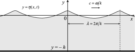
Fig. 1.: Sketch of the physical domain occupied by an ideal incompressible fluid of finite depth

Consider a modulated wavetrain with carrier frequency $\omega$ and wavenumber $k$.  In this case, a solution to Eqs.  (3)–(6) can be looked for in the form of Fourier series with variable coefficients:

$$\begin{array}[]{l}\displaystyle\!\left(\!\!\begin{array}[]{c}\Phi(x,\,y,\,t)\\ \eta(x,\,t)\end{array}\!\!\right)=\sum_{n=-\infty}^{\infty}\left(\!\!\begin{array}[]{c}\Phi_{n}(x,\,y,\,t)\\ \eta_{n}(x,\,t)\end{array}\!\!\right)\mathrm{e}^{\texttt{i}n(kx-\omega t)},\\[14.22636pt] \displaystyle\eta_{-n}\equiv\eta_{n}^{*},\;\;\Phi_{-n}\equiv\Phi_{n}^{*},\end{array}\!\!\!\!\!\!\!\!\!\!\!\!\!\!\!\!\!\!\!\!$$ (7)

where ^∗ stands for complex conjugate (here, we assume the carrier wave to be symmetric), the functions $\Phi(x,\,y,\,t)$ and $\eta(x,\,t)$ are assumed to be real by definition. Substituting (7) in (3)–(6) and equating the coefficients at the like powers of $\exp(\texttt{i}(kx-\omega t))$, one can obtain a system of nonlinear partial differential equations for the functions $\Phi_{n}(x,\,y,\,t)$ and $\eta_{n}(x,\,t)$.  Linearization of these equations at $n=1$ gives the dispersion relation for gravity waves:

$$\omega^{2}=gk\tanh(kh).$$ (8)

3 Slowly Modulated Quasi-Harmonic Wavetrains and Multiple-Scale Expansions

Generally the system of equations for $\Phi_{n}(x,\,y,\,t)$ and $\eta_{n}(x,\,t)$ is by no means more simple than original equations.  It can be simplified when solutions are looked for in a class of functions with narrow spectrum, $|\Delta k|\ll k$.  In this case, the problem has a formal small parameter $\mu\sim|\Delta k|\bigl{/}k$ (quasi-monochromaticity condition), with $\Phi_{n}(x,\,y,\,t)$ and $\eta_{n}(x,\,t)$ being slow functions of $x$ and $t$.  Accordingly, the wave motion can be classified into slow one and fast one by introducing different time scales and different spatial scales:

$$T_{n}\equiv\mu^{n}t,\quad X_{n}\equiv\mu^{n}x.$$ (9)

The derivatives with respect to time and coordinate are expanded into the following series:

$$\frac{\partial}{\partial t}=\sum_{n=0}^{\infty}\mu^{n}\frac{\partial}{\partial T_{n}},\qquad\frac{\partial}{\partial x}=\sum_{n=0}^{\infty}\mu^{n}\frac{\partial}{\partial X_{n}},$$ (10)

the times $T_{n}$ and coordinates $X_{n}$ being assumed to be independent variables.

When there are no resonances between higher harmonics, the amplitudes of Fourier coefficients decrease with increasing number (quasi-harmonicity condition):

$$\eta_{n}\sim\varepsilon^{n}A,\quad n\geqslant 1,\quad\eta_{0}\sim\varepsilon^{2}A,\quad\varepsilon<1,$$ (11)

where

$$\eta_{1}\equiv\frac{1}{2}\varepsilon A(x,\,t).$$ (12)

The parameter $\varepsilon$ can be regarded as a formal small parameter related to the smallness of wave amplitude as compared to the carrier wavelength $\lambda\equiv\frac{2\pi}{k}$.  In this case, the unknown functions $\Phi_{n}(x,\,y,\,t)$ and $\eta_{n}(x,\,t)$ can be expanded into power series in the formal parameter $\varepsilon$:

$$\left(\!\!\!\begin{array}[]{c}\Phi_{n}(x,\,y,\,t)\\ \eta_{n}(x,\,t)\end{array}\!\!\!\right)=\sum_{m=1}^{\infty}\varepsilon^{m}\left(\!\!\begin{array}[]{c}\Phi_{n}^{(m)}(x,\,y,\,t)\\ \eta_{n}^{(m)}(x,\,t)\end{array}\!\!\!\right)\!\!.$$ (13)

Multiple-scale expansions (10) and (13) allow the functions $\Phi_{n}(x,\,y,\,t)$ and $\eta_{n}(x,\,t)$ to be expressed in terms of the first harmonic envelope $A(x,\,t)$, as described in detail in [47].  Note that in the procedure described in [47] it is essential to set $\varepsilon\equiv\mu$.

In practice, the quasi-harmonicity condition can be written as

$$|k\eta_{1}|\ll 1,$$ (14)

and the condition of slow modulation (quasi-monochromaticity) can be formalized as

$$\left|\frac{A_{x}}{kA}\right|\ll 1,$$ (15)

which follows from differentiating the function $A(x,\,t)\exp\bigl{(}\texttt{i}(kx-\omega t)\bigr{)}$ with respect to $x$.  With these conditions satisfied, the original system of equations (3)–(6) can be reduced to one evolution equation for the first harmonic envelope $A(x,\,t)$ with the use of small-amplitude expansions (10) and (13).

4 High-Order
Nonlinear Schrödinger Equation

4.1 Equation derived by Sedletsky

Sedletsky [47,​ 48] used the above-described multiple-scale procedure to derive the following HONLSE for the first-harmonic envelope $A(x,\,t)$ (Eq.  (68) in [47]):

$$\texttt{i}\left(\!\frac{\partial A}{\partial(\varepsilon t)}+V_{g}\frac{\partial A}{\partial(\varepsilon x)}\!\right)+$$

$$+\,\varepsilon\left(\!\frac{1}{2}\omega^{\prime\prime}\frac{\partial^{2}A}{\partial(\varepsilon x)^{2}}+\omega k^{2}q_{3}|A|^{2}A\!\right)+$$

$$+\,\texttt{i}\varepsilon^{2}\biggl{(}\!-\frac{1}{6}\omega^{\prime\prime\prime}\frac{\partial^{3}A}{\partial(\varepsilon x)^{3}}+\omega kQ_{41}|A|^{2}\frac{\partial A}{\partial(\varepsilon x)}\,+$$

$$+\,\omega kQ_{42}A^{2}\frac{\partial A^{*}}{\partial(\varepsilon x)}\!\biggr{)}=0\;\;[\text{m}/\text{s}].$$ (16)

As compared to the standard NLSE, this equation takes into account additional nonlinear and dispersive terms of order $\mathcal{O}(\varepsilon^{2})$.  Equation (16) was later re-derived by Slunyaev [52], who confirmed the symbolic computations presented in [47,​ 48] and extended them to the $\mathcal{O}(\varepsilon^{3})$ order.  Here, we restrict our attention to the original equation (16).  The parameters of this equation are given by

$$\omega=\left(gk\sigma\right)^{1/2},\quad\sigma\equiv\tanh(kh),$$ (17a)

$$\omega^{\prime}=\frac{\partial\omega}{\partial k}\equiv V_{g}=\frac{\omega}{2k}\left(\!1+\frac{2kh}{\sinh(2kh)}\!\right)=$$

$$=\frac{\omega}{2k}\left(\!1+\frac{1-\sigma^{2}}{\sigma}kh\!\right)\!\!,$$ (17b)

$$\omega^{\prime\prime}=\frac{\partial^{2}\omega}{\partial k^{2}}=\frac{\omega}{4k^{2}\sigma^{2}}\Bigl{(}\!\left(\sigma^{2}-1\right)\left(3\sigma^{2}+1\right)k^{2}h^{2}\,-$$

$$-\,2\sigma\left(\sigma^{2}-1\right)kh-\sigma^{2}\!\Bigr{)}\!,$$ (17c)

$$\omega^{\prime\prime\prime}=\frac{\partial^{3}\omega}{\partial k^{3}}=-\frac{\omega}{8k^{3}\sigma^{3}}\Bigl{(}\!\left(\sigma^{2}-1\right)\times$$

$$\times\left(15\sigma^{4}\!-2\sigma^{2}+3\right)k^{3}h^{3}\!-3\sigma\left(\sigma^{2}\!-1\right)\!\left(3\sigma^{2}\!+1\right)k^{2}h^{2}\,-$$

$$-\,3\sigma^{2}\left(\sigma^{2}-1\right)kh-3\sigma^{3}\!\Bigr{)}\!,$$ (17d)

$$q_{3}=-\frac{1}{16\sigma^{4}\nu}\Bigl{(}\!\left(\sigma^{2}-1\right)^{2}\left(9\sigma^{4}-10\sigma^{2}+9\right)k^{2}h^{2}\,+$$

$$+\,2\sigma\left(3\sigma^{6}-23\sigma^{4}+13\sigma^{2}-9\right)kh\,-$$

$$-\,\sigma^{2}\left(7\sigma^{4}-38\sigma^{2}-9\right)\!\Bigr{)}\!,$$ (17e)

$$Q_{41}=\frac{1}{32\sigma^{5}\nu^{2}}\Bigl{(}\!\left(\sigma^{2}-1\right)^{5}\times$$

$$\times\left(3\sigma^{6}-20\sigma^{4}-21\sigma^{2}+54\right)k^{5}h^{5}\,-$$

$$-\,\sigma\left(\sigma^{2}\!-1\right)^{3}\bigl{(}11\sigma^{8}\!-99\sigma^{6}\!-61\sigma^{4}\!+7\sigma^{2}\!+270\bigr{)}k^{4}h^{4}\,+$$

$$+\,2\sigma^{2}\left(\sigma^{2}-1\right)\bigl{(}7\sigma^{10}-58\sigma^{8}+38\sigma^{6}+52\sigma^{4}\,-$$

$$-\,181\sigma^{2}+270\!\bigr{)}k^{3}h^{3}-2\sigma^{3}\bigl{(}3\sigma^{10}+18\sigma^{8}-146\sigma^{6}\,-$$

$$-\,172\sigma^{4}+183\sigma^{2}-270\bigr{)}k^{2}h^{2}-\sigma^{4}\bigl{(}\sigma^{8}-109\sigma^{6}+517\sigma^{4}\,+$$

$$+\,217\sigma^{2}+270\bigr{)}kh+\sigma^{5}\left(\sigma^{6}-40\sigma^{4}+193\sigma^{2}+54\right)\!\Bigr{)}+\Delta,$$ (17f)

$$Q_{42}=\frac{1}{32\sigma^{5}\nu^{2}}\Bigl{(}\!-\left(\sigma^{2}-1\right)^{5}\times$$

$$\times\left(3\sigma^{6}+7\sigma^{4}-11\sigma^{2}+9\right)k^{5}h^{5}\,+$$

$$+\,\sigma\left(\sigma^{2}\!-1\right)^{3}\left(11\sigma^{8}\!-48\sigma^{6}\!+66\sigma^{4}\!+8\sigma^{2}\!+27\right)k^{4}h^{4}\,-$$

$$-\,2\sigma^{2}\left(\sigma^{2}-1\right)\bigl{(}7\sigma^{10}-79\sigma^{8}+282\sigma^{6}\,-$$

$$-\,154\sigma^{4}-\sigma^{2}+9\bigr{)}k^{3}h^{3}+2\sigma^{3}\bigl{(}3\sigma^{10}-63\sigma^{8}+314\sigma^{6}\,-$$

$$-\,218\sigma^{4}+19\sigma^{2}+9\bigr{)}k^{2}h^{2}+\sigma^{4}\bigl{(}\sigma^{8}+20\sigma^{6}-158\sigma^{4}\,-$$

$$-\,28\sigma^{2}-27\bigr{)}kh-\sigma^{5}\left(\sigma^{6}-7\sigma^{4}+7\sigma^{2}-9\right)\!\Bigr{)}-\Delta,$$ (17g)

$$\nu=\left(\sigma^{2}-1\right)^{2}k^{2}h^{2}-2\sigma\left(\sigma^{2}+1\right)kh+\sigma^{2}.$$ (17h)

The quantity $V_{g}$ is the wave group speed.  The parameter $\Delta$ is the correction introduced by Slunyaev [52] to the coefficients derived in [47,​ 48].  This correction is negligible at $kh\gtrsim 1$ (see Appendix A), and we ignore it by keeping $\Delta=0$.

The free-surface displacement is expressed in terms of $A$ as

$$\eta=\varepsilon^{2}\eta_{0}+\varepsilon\mathop{\rm Re}\nolimits\bigl{(}A\mathrm{e}^{\texttt{i}(kx-\omega t)}\bigr{)}\,+$$

$$+\,\varepsilon^{2}\,2\mathop{\rm Re}\nolimits\bigl{(}\eta_{2}\,\mathrm{e}^{2\texttt{i}(kx-\omega t)}\bigr{)}+\mathcal{O}(\varepsilon^{3}),$$ (18)

where $\mathop{\rm Re}\nolimits\{\cdot\}$ stands for the real part of a complex-valued function.  Here, $\eta_{0}$ and $\eta_{2}$ are defined as

$$\eta_{0}=\frac{\sigma+2\left(1-\sigma^{2}\right)kh}{\nu}\,k|A|^{2},$$ (19a)

$$\eta_{2}=\frac{3-\sigma^{2}}{8\sigma^{3}}\,kA^{2}.$$ (19b)

The corresponding velocity potential is written as

$$\Phi=\varepsilon\Phi_{0}+\varepsilon\,2\mathop{\rm Re}\nolimits\bigl{(}\Phi_{1}\,\mathrm{e}^{\texttt{i}(kx-\omega t)}\bigr{)}\,+$$

$$+\,\varepsilon^{2}\,2\mathop{\rm Re}\nolimits\bigl{(}\Phi_{2}\,\mathrm{e}^{2\texttt{i}(kx-\omega t)}\bigr{)}+\mathcal{O}(\varepsilon^{3}),$$ (20)

where

$$\Phi_{1}=\frac{\omega}{2k\sigma}\Biggl{(}\!\biggl{(}\!\frac{\partial A}{\partial x}\biggl{(}h\sigma+\frac{V_{g}}{\omega}\biggr{)}-\texttt{i}A\!\biggr{)}\frac{\cosh\bigl{(}k(y+h)\bigr{)}}{\cosh(kh)}\,-$$

$$-\,(y+h)\frac{\partial A}{\partial x}\,\frac{\sinh\bigl{(}k(y+h)\bigr{)}}{\cosh(kh)}\!\Biggr{)}\!,$$ (21a)

$$\Phi_{2}=3\texttt{i}\omega\,\frac{(\sigma^{4}-1)}{16\sigma^{4}}\,\frac{\cosh\bigl{(}2k(y+h)\bigr{)}}{\cosh(2kh)}\,A^{2}.$$ (21b)

The term $\Phi_{0}$ describes the wave-induced mean flow and is expressed implicitly in terms of its derivatives

$$\frac{\partial\Phi_{0}}{\partial x}=\varepsilon\frac{\omega k\gamma_{1}}{2\sigma\nu}|A|^{2}+\texttt{i}\varepsilon\frac{\omega\gamma_{2}}{8\sigma^{2}\nu^{2}}\left(\!A\frac{\partial A^{*}}{\partial x}-A^{*}\frac{\partial A}{\partial x}\!\right)\!\!,$$ (22a)

$$\frac{\partial\Phi_{0}}{\partial t}=-V_{g}\frac{\partial\Phi_{0}}{\partial x},$$ (22b)

where

$$\gamma_{1}=\bigl{(}\sigma^{2}-1\bigr{)}^{2}kh-\sigma\bigl{(}\sigma^{2}-5\bigr{)},$$ (23a)

$$\gamma_{2}=\bigl{(}\sigma^{2}-1\bigr{)}^{5}k^{4}h^{4}+4\sigma\bigl{(}\sigma^{2}-1\bigr{)}^{2}\bigl{(}13\sigma^{2}+3\bigr{)}k^{3}h^{3}\,-$$

$$-\,2\sigma^{2}\bigl{(}\sigma^{2}-1\bigr{)}\bigl{(}3\sigma^{4}+32\sigma^{2}-3\bigr{)}k^{2}h^{2}\,+$$

$$+\,4\sigma^{3}\bigl{(}2\sigma^{4}-\sigma^{2}-5\bigr{)}kh-3\sigma^{4}\bigl{(}\sigma^{2}-5\bigr{)}.$$ (23b)

Functions (18) and (20) define an approximate solution to the original system of equations (3)–(6) in terms of the first-harmonic envelope $A$, which is found from Eq. (16).

4.2 Dimensionless form

Fig. 2.: $\omega^{\prime\prime}$ in $\mathrm{m}^{2}/\mathrm{s}$ as a function of $h$ at $k=1$ and $g=9.8\,\mathrm{m}/\mathrm{s}^{2}$

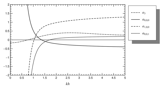
Fig. 3.: Normalized coefficients of HONLSE as functions of $kh$                                

Introduce the following dimensionless time, coordinate, and amplitude:

$$\tau=\beta t,\quad\chi=kx,\quad u=\alpha^{-1}\varepsilon A,$$ (24)

$\alpha$ and $\beta$ being the parameters to be determined.  The relationship between the old and new derivatives is

$$\frac{\partial}{\partial x}=k\frac{\partial}{\partial\chi},\quad\frac{\partial}{\partial t}=\beta\frac{\partial}{\partial\tau}.$$

Then Eq. (16) is transformed to

$$\texttt{i}\alpha\left(\beta u_{\tau}+kV_{g}u_{\chi}\right)+\alpha\left(\!\frac{1}{2}\omega^{\prime\prime}k^{2}u_{\chi\chi}+\omega k^{2}q_{3}|\alpha|^{2}|u|^{2}u\!\right)+$$

$$+\,\texttt{i}\alpha\Bigl{(}-\frac{1}{6}\omega^{\prime\prime\prime}k^{3}u_{\chi\chi\chi}+\omega k^{2}Q_{41}|\alpha|^{2}u_{\chi}|u|^{2}\,+$$

$$+\,\omega k^{2}Q_{42}|\alpha|^{2}u^{2}u^{*}_{\chi}\Bigr{)}=0\;\;[\text{m}/\text{s}].$$

Here, the indices $\chi$ and $\tau$ designate the partial derivatives with respect to the corresponding variables.  Taking into account that $\omega^{\prime\prime}<0$ at all $h>0$ (Fig.  2), divide this equation by $\omega^{\prime\prime}k^{2}\alpha$ so that

$$\texttt{i}\left(\!\frac{\beta}{\omega^{\prime\prime}k^{2}}u_{\tau}+\frac{V_{g}}{\omega^{\prime\prime}k}u_{\chi}\!\right)+\left(\!\frac{1}{2}u_{\chi\chi}+\frac{\omega}{\omega^{\prime\prime}}|\alpha|^{2}q_{3}|u|^{2}u\!\right)+$$

$$+\,\texttt{i}\Bigl{(}\!-\frac{1}{6}\frac{\omega^{\prime\prime\prime}k}{\omega^{\prime\prime}}u_{\chi\chi\chi}+\frac{\omega}{\omega^{\prime\prime}}|\alpha|^{2}Q_{41}u_{\chi}|u|^{2}\,+$$

$$+\,\frac{\omega}{\omega^{\prime\prime}}|\alpha|^{2}Q_{42}u^{2}u^{*}_{\chi}\!\Bigr{)}=0$$

and select the values of $\alpha$ and $\beta$ as

$$|\alpha|^{2}=-\frac{\omega^{\prime\prime}}{\omega}>0,\quad\beta=-\omega^{\prime\prime}k^{2}>0.$$ (25)

Thus, Eq.  (16) takes the dimensionless form

$$\texttt{i}\left(\!u_{\tau}-\frac{V_{g}}{\omega^{\prime\prime}k}u_{\chi}\!\right)-\frac{1}{2}u_{\chi\chi}+q_{3}|u|^{2}u\,+$$

$$+\,\texttt{i}\left(\!\frac{1}{6}\frac{\omega^{\prime\prime\prime}k}{\omega^{\prime\prime}}u_{\chi\chi\chi}+Q_{41}u_{\chi}|u|^{2}+Q_{42}u^{2}u^{*}_{\chi}\!\right)=0$$

or, equivalently,

$$\texttt{i}\bigl{(}u_{\tau}+a_{1}u_{\chi}\bigr{)}-a_{2}u_{\chi\chi}+a_{0,\,0,\,0}|u|^{2}u+\texttt{i}\Bigl{(}-a_{3}u_{\chi\chi\chi}\,+$$

$$+\,a_{1,\,0,\,0}u_{\chi}|u|^{2}+a_{0,\,0,\,1}u^{2}u^{*}_{\chi}\Bigr{)}=0,$$ (26a)

which finally yields

$$u_{\tau}=-a_{1}u_{\chi}-\texttt{i}a_{2}u_{\chi\chi}+\texttt{i}a_{0,\,0,\,0}|u|^{2}u\,+$$

$$+\,\Bigl{(}a_{3}u_{\chi\chi\chi}-a_{1,\,0,\,0}u_{\chi}|u|^{2}-a_{0,\,0,\,1}u^{2}u^{*}_{\chi}\Bigr{)}\!,$$ (26b)

where we used the unified notation introduced by Lukomsky and Gandzha [42]. Here, the coefficients

$$\begin{array}[]{l}\displaystyle a_{1}=-\frac{V_{g}}{\omega^{\prime\prime}k}=-\frac{2}{\upsilon}\Bigl{(}\!\sigma^{2}+\sigma\left(1-\sigma^{2}\right)kh\!\Bigr{)}>0,\\[8.53581pt] \displaystyle a_{2}=\frac{1}{2},\\[8.53581pt] \displaystyle a_{3}\equiv-\frac{1}{6}\frac{\omega^{\prime\prime\prime}k}{\omega^{\prime\prime}}=\\[8.53581pt] \displaystyle=\frac{1}{12\sigma\upsilon}\Bigl{(}\!\left(\sigma^{2}-1\right)\left(15\sigma^{4}-2\sigma^{2}+3\right)k^{3}h^{3}\,-\\[8.53581pt] \displaystyle-\,3\sigma\left(\sigma^{2}-1\right)\left(3\sigma^{2}+1\right)k^{2}h^{2}\,-\\[2.84526pt] \displaystyle-\,3\sigma^{2}\left(\sigma^{2}-1\right)kh-3\sigma^{3}\!\Bigr{)}\!,\\[2.84526pt] \displaystyle a_{0,\,0,\,0}\equiv q_{3},\quad a_{1,\,0,\,0}\equiv Q_{41},\quad a_{0,\,0,\,1}\equiv Q_{42},\\[2.84526pt] \displaystyle\upsilon=\left(\sigma^{2}-1\right)\left(3\sigma^{2}+1\right)k^{2}h^{2}-2\sigma\left(\sigma^{2}-1\right)kh-\sigma^{2}\end{array}\!\!\!\!\!\!\!\!\!\!\!\!\!\!\!\!\!\!\!\!\!\!\!\!$$ (27)

are all real and depend on one dimensionless parameter $kh$.  Their behavior as functions of $kh$ is shown in Fig.  3.  It can be seen that Eq.  (16) is valid at $kh\gtrsim 1$, where the coefficients $a_{0,\,0,\,0}$, $a_{1,\,0,\,0}$, and $a_{0,\,0,\,1}$ do not diverge.  At smaller depths, the Korteweg–de Vries equation and its generalizations [36,​ 39] should be used.  On the other hand, at large $kh$, the infinite-depth limit (Dysthe’s equation) should be used.  Indeed, the following asymptotics are easily obtained at $kh\rightarrow\infty$:

$$a_{3}=\frac{1}{4},\;a_{0,\,0,\,0}=-\frac{1}{2},\;a_{1,\,0,\,0}=\frac{3}{2},\;a_{0,\,0,\,1}=\frac{1}{4}.\!\!\!\!$$ (28)

They coincide with the corresponding coefficients of Dysthe’s equation [63], except for the term including the wave-induced mean flow, which cannot be explicitly reconstructed from Eq.  (26) because of the additional power expansion of the wave-induced mean flow made to derive Eq.  (16).  However, this term can be reconstructed from the equations generating Eq.  (16), at the stage when the wave-induced mean flow has not been excluded from the equation for $A$ yet [47].  Taking into account these constraints, we will restrict our attention to the following range of intermediate depths:

$$1<kh<5.$$ (29)

4.3 Moving reference frame

Equation (26) can be rewritten in the form without the $u_{\chi}$ term.  To this end, let us proceed to the reference frame moving with speed $a_{1}$ (dimensionless group speed):

$$\xi=\chi-a_{1}\tau,\quad T=\tau.$$ (30)

The relationship between the derivatives in new and old variables is given by the formulas

$$\frac{\partial}{\partial\chi}=\frac{\partial\xi}{\partial\chi}\frac{\partial}{\partial\xi}+\frac{\partial T}{\partial\chi}\frac{\partial}{\partial T}=\frac{\partial}{\partial\xi},$$

$$\frac{\partial}{\partial\tau}=\frac{\partial\xi}{\partial\tau}\frac{\partial}{\partial\xi}+\frac{\partial T}{\partial\tau}\frac{\partial}{\partial T}=-a_{1}\frac{\partial}{\partial\xi}+\frac{\partial}{\partial T},$$

so that

$$u_{\tau}=-\texttt{i}a_{2}u_{\xi\xi}+\texttt{i}a_{0,\,0,\,0}|u|^{2}u\,+$$

$$+\,\Bigl{(}\!a_{3}u_{\xi\xi\xi}-a_{1,\,0,\,0}u_{\xi}|u|^{2}-a_{0,\,0,\,1}u^{2}u^{*}_{\xi}\!\Bigr{)}\!.$$ (31)

This is our target equation for numerical simulations.  It possesses the integral of motion

$$I_{0}(\tau)=\int\limits_{-\infty}^{\infty}|u(\xi,\,\tau)|^{2}\mathrm{d}\xi=\mathrm{const},$$ (32)

which expresses the conservation of wave action.  The derivation of this conservation law is given in Appendix C.  It allows one to trace the relative numerical error of simulations:

$$\mathrm{Er}(I_{0})=\frac{|I_{0}(\tau)-I_{0}(0)|}{I_{0}(0)}.$$ (33)

Fig. 4.: Ratio between the dimensionless phase and group speeds as a function of $kh$

Of particular interest is to reveal any relationship of Eq.  (31) to other HONLSEs derived in different contexts.  In Appendix B, we consider one such equation (the Sasa–Satsuma equation) and prove that Eq.  (31) cannot be reduced to it at any $kh$.

4.4 Dimensionless free surface
displacement and velocity potential

The dimensionless free surface displacement is expressed in terms of $u$ as follows:

$$\zeta\equiv k\eta=\alpha_{0}|u|^{2}+\alpha_{1}\mathop{\rm Re}\nolimits\bigl{(}u\,\mathrm{e}^{\texttt{i}\theta}\bigr{)}+2\alpha_{2}\mathop{\rm Re}\nolimits\bigl{(}u^{2}\,\mathrm{e}^{2\texttt{i}\theta}\bigr{)},$$ (34)

$$\alpha_{0}=\frac{\sigma+2\left(1-\sigma^{2}\right)kh}{c\nu},\quad\alpha_{1}=\frac{1}{\sqrt{c}},\quad\alpha_{2}=\frac{3-\sigma^{2}}{8c\sigma^{3}},$$

where

$$\theta=kx-\omega t=\chi-c\tau=\xi+\left(a_{1}-c\right)\tau$$ (35)

is the wave phase and

$$c=\frac{1}{|\alpha|^{2}k^{2}}=-\frac{4\sigma^{2}}{\upsilon}$$ (36)

is the dimensionless phase speed.  Figure 4 shows the ratio of the phase speed $c$ to the group speed $a_{1}$ as a function of $kh$.  This ratio is equal to unity at $kh\rightarrow 0$, and it is twice as large at $kh\rightarrow\infty$, in full conformity with the classical water wave theory [24].  The wave envelope is written as

$$\left[\zeta\right]_{\mathrm{envelope}}=\alpha_{1}|u|+\left(\alpha_{0}+2\alpha_{2}\right)|u|^{2}.$$ (37)

The corresponding dimensionless velocity potential is expressed as

$$\varphi\equiv-\frac{1}{\omega^{\prime\prime}}\Phi=\varphi_{0}+2\mathop{\rm Re}\nolimits\bigl{(}\varphi_{1}\,\mathrm{e}^{\texttt{i}\theta}\bigr{)}\,+$$

$$+\,2\mathop{\rm Re}\nolimits\bigl{(}\varphi_{2}\,\mathrm{e}^{2\texttt{i}\theta}\bigr{)},$$ (38)

$$\left(\varphi_{0}\right)_{\xi}=\frac{\gamma_{1}}{2\sigma\nu}|u|^{2}+\frac{\texttt{i}\gamma_{2}}{8\sigma^{2}\nu^{2}}\left(uu^{*}_{\xi}-u^{*}u_{\xi}\right)\!,$$

$$\left(\varphi_{0}\right)_{\tau}=-a_{1}\left(\varphi_{0}\right)_{\xi},$$

$$\varphi_{1}=\frac{\sqrt{c}}{2\sigma}\Biggl{(}\!\!\biggl{(}\!-\texttt{i}u+\frac{\bigl{(}\sigma^{2}+1\bigr{)}kh+\sigma}{2\sigma}\,u_{\xi}\!\biggr{)}\times$$

$$\times\,\frac{\cosh(z+kh)}{\cosh(kh)}-(z+kh)\frac{\sinh(z+kh)}{\cosh(kh)}\,u_{\xi}\!\Biggr{)}\!,$$

$$\varphi_{2}=\frac{3\texttt{i}\bigl{(}\sigma^{4}-1\bigr{)}}{16\sigma^{4}}\,\frac{\cosh(2(z+kh)\bigr{)}}{\cosh(2kh)}\,u^{2},$$

where $z\equiv ky$ is the dimensionless vertical coordinate.  The quasi-harmonicity condition is written as

$$\frac{|u|}{\sqrt{c}}\ll 1,$$ (39)

and the quasi-monochromaticity condition is

$$\left|\frac{u_{\xi}}{u}\right|\ll 1.$$ (40)

Finally, the original equations of hydrodynamics can be written in the following dimensionless form:

$$\varphi_{\xi\xi}+\varphi_{zz}=0,\leavevmode\nobreak\ -\infty<\xi<\infty,\leavevmode\nobreak\ \displaystyle-kh<z<\zeta(\xi,\,\tau);$$ (41)

$$\varphi_{\tau}+\frac{1}{2}\bigl{(}\varphi_{\xi}^{2}+\varphi_{z}^{2}\bigr{)}+\frac{c^{2}}{\sigma}\,\zeta=0,\leavevmode\nobreak\ \leavevmode\nobreak\ \leavevmode\nobreak\ z=\zeta(\xi,\,\tau);$$ (42)

$$\zeta_{\,\tau}-\varphi_{z}+\zeta_{\,\xi}\,\varphi_{\xi}=0,\leavevmode\nobreak\ \leavevmode\nobreak\ \leavevmode\nobreak\ z=\zeta(\xi,\,\tau);$$ (43)

$$\varphi_{z}=0,\leavevmode\nobreak\ \leavevmode\nobreak\ \leavevmode\nobreak\ z=-kh.$$ (44)

5 Numerical Simulations

In this section, we adopt the split-step Fourier (SSF) technique described in Appendix D to compute solutions to HONLSE (31).  To test the accuracy of our numerical scheme, we start from classical NLSE (1) written in terms of the coordinate $\xi$.  At $a_{0,\,0,\,0}<0$ ($kh\gtrsim 1.363$), it has an exact one-soliton solution [69]:

$$u(\xi,\,\tau)=\frac{u_{0}\exp\left(\texttt{i}\kappa\xi-\texttt{i}\Omega\tau\right)}{\cosh\bigl{(}K(\xi-\xi_{0}-V\tau)\bigr{)}},$$ (45)

$$\Omega=\left(K^{2}-\kappa^{2}\right)a_{2},\;V=-2\kappa a_{2},\;K=|u_{0}|\sqrt{-\frac{a_{0,\,0,\,0}}{2a_{2}}},$$

$$u_{0}\in\mathds{C},\quad\kappa,\;\xi_{0}\in\mathds{R}.$$

Here, $V$ is the soliton speed, $u_{0}$ is the complex amplitude, $\kappa$ and $\Omega$ are the soliton’s wavenumber and frequency, and $\xi_{0}$ is the soliton’s initial position.  The amplitude $u_{0}$ and wavenumber $\kappa$ should be selected such that the quasi-harmonicity and quasi-monochromaticity conditions (39), (40) hold true.  In practice, these conditions mean that the soliton amplitude and wavenumber should be small:

$$|u_{0}|\ll 1,\quad\kappa\ll 1.$$

In this study, we restrict our attention by the following choice of parameters:

$$u_{0}=0.1,\quad\kappa=-K\;(\Rightarrow\;\Omega=0),\quad\xi_{0}=0.$$ (46)

Figures 5 and 6 demonstrate that constraints (39) and (40) are readily satisfied in this case.  Note that at $\kappa<0$ we have $V>0$. In this case, solitons move from left to right with speed exceeding the carrier group speed.

Figure 7 shows a soliton computed for $kh=3$ using analytical formula (45) for the initial moment $\tau=0$ and moment $\tau=10000$.  The same soliton was taken as the initial condition for the simulation with the SSF technique.  The deviation from the exact solution is seen to be negligible.  Indeed, the numerical error estimated with formula (33) is

$$S^{(2)}|_{\tau=10000}:\leavevmode\nobreak\ \leavevmode\nobreak\ \mathrm{Er}(I_{0})=1.3\times 10^{-10}\%,$$

$$\Delta_{\mathrm{rms}}(u_{\mathrm{exact}},\,u_{\mathrm{comp}})=1.0\times 10^{-4}\%,$$

$$S^{(4)}|_{\tau=10000}:\leavevmode\nobreak\ \leavevmode\nobreak\ \mathrm{Er}(I_{0})=2.3\times 10^{-10}\%,$$

$$\Delta_{\mathrm{rms}}(u_{\mathrm{exact}},\,u_{\mathrm{comp}})=3.5\times 10^{-9}\%,$$

where $S^{(2)}$ and $S^{(4)}$ designate the order of the SSF technique adopted for calculation (see Appendix D) and

$$\Delta_{\mathrm{rms}}(u,\,g)(\tau)=\sqrt{\frac{\int_{-\infty}^{\infty}\left(|u(\xi,\,\tau)|-|g(\xi,\,\tau)|\right)^{2}\mathrm{d}\xi}{I_{0}}}$$

is the relative r.m.s. deviation between two functions.  Thus, our numerical scheme reproduces the exact one-soliton solution to NLSE with high accuracy.

Figure 8 shows the evolution of the same one-soliton waveform taken as the initial condition in HONLSE (31).  As compared to the NLSE case, the wave amplitude is smaller, the pulse width is larger, and the wave speed is higher. The wave amplitude does not remain constant and exhibits slow oscillations that can be interpreted as the secondary modulation of the carrier wave.  The amplitude of these oscillations decreases with time (Fig.  9).  Such a solution does not fall under the definition of soliton because it does not preserve the constant amplitude and shape during the evolution.  On the other hand, it moves with nearly the constant speed (Fig.  10) and still possesses the unique property of solitons to exist over long periods of time without breaking.  In view of this unique property, we call such solutions quasi-solitons. The term quasi-soliton was introduced earlier by Zakharov and Kuznetsov [70], but in somewhat different context; then Karpman et al.  [38] and Slunyaev [53] used it in the same context as in the present study.

Fig. 5.: Testing the quasi-harmonicity condition (39) for $kh=3$

Fig. 6.: Testing the quasi-monochromaticity condition (40) for $kh=3$

Fig. 7.: Evolution of one-soliton solution (45) to NLSE (1) at $kh=3$.  SSF parameters: $\Delta\tau=1,\;\Delta\xi=2,\;\xi\in[-1000,\,1000);\;V\approx 0.0566$

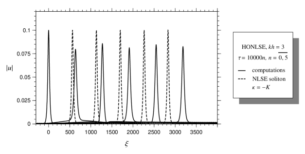
Fig. 8.: Evolution of one-soliton waveform (45) taken as the initial condition in HONLSE (31) at $kh=3$.  SSF parameters: $\Delta\tau=0.5,\;\Delta\xi=2,\;\xi\in[-4000,\,4000)$.  Accuracy: $S^{(2)}|_{\tau=50000}$: $\mathrm{Er}(I_{0})=0.050$%

Fig. 9.: Variations in the amplitude of the quasi-soliton solution with distance at $kh=3$

Fig. 10.: Mean wave speed as a function of distance at $kh=3$: solid curve — quasi-soliton, dashed line — NLSE soliton ($V\approx$ $\approx 0.0566$)

Fig. 11.: Evolution of one-soliton waveform (45) taken as the initial condition in HONLSE (31) at $kh=2$.  SSF parameters: $\Delta\tau=0.5,\;\Delta\xi=2,\;\xi\in[-4000,\,4000)$. Accuracy: $S^{(2)}|_{\tau=60000}:\;\mathrm{Er}(I_{0})=0.028\%$

Such a behavior of NLSE solitons in the HONLSE case was first described by Akylas [3] in the context of asymptotic modeling and numerical simulations of Dysthe’s equation in the infinite-depth limit.  Growth in the soliton speed corresponds to the well-known carrier frequency downshift observed in deep-water experiments by Su [60] and in simulations of Dysthe’s equation by Lo and Mei [40].  Dysthe [19] pointed out that this phenomenon originates due to the wave-induced mean flow, whose component in the direction of propagation of the wave causes a local Doppler shift.  Here, we proved for the first time that this well-known phenomenon can be observed on finite depth as well.  This result is the main practical achievement of our study.  Figures  11, 12, and 13 demonstrate that the same quasi-soliton solution and frequency downshift are observed at a smaller depth, $kh=2$.

Fig. 12.: Variations in the amplitude of the quasi-soliton solution with distance at $kh=2$

Fig. 13.: Mean wave speed as a function of distance at $kh=2$: solid curve – quasi-soliton, dashed line – NLSE soliton ($V\approx$ $\approx 0.0469$)

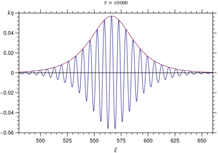
Fig. 14.: Free surface profile with envelope in the form of quasi-soliton at $kh=3$

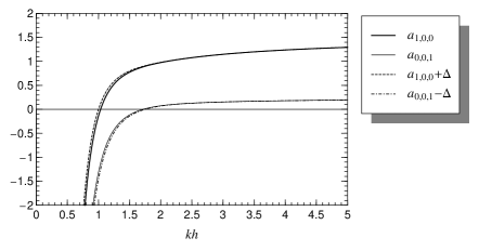
Fig. 15.: Effect of correction $\Delta$ on the coefficients $a_{1,\,0,\,0}$ and $a_{0,\,0,\,1}$

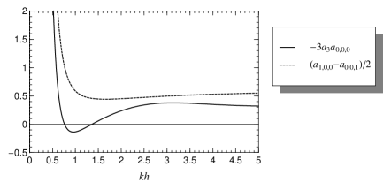
Fig. 16.: The left- and right-hand-sides of Eq. (2) versus $kh$

Finally, the free surface profile reconstructed with formula (34) is shown in Fig. 14 for $kh=3$. The dimensionless maximum free surface elevation is about $0.046$. The case $kh=3$ corresponds to wavelengths twice as large as depth, $\lambda\approx 2h$.  The typical depth of the shelf near the north-west shore of the Black Sea varies from 10 to 100 m.  Hence, the wavelength corresponding to $kh=3$ falls within the range from 20 to 200 m, which is quite typical of water waves observed on the Black Sea.  For $h=30$ m, we have $\lambda\approx 60$ m and $k=0.1\;\mathrm{m}^{-1}$.  The corresponding maximum free surface elevation of the wave shown in Fig. 14 is about $0.5$ m, and the significant wavetrain width is about 2 km.  Thus, quasi-soliton solutions obtained in this study can describe swells propagating on the relatively calm background on seas with intermediate depths.  The typical trough-to-crest height of such swells is about 1 m.

6 Conclusions

The HONLSE derived earlier by Sedletsky [47] for the first-harmonic envelope of slowly modulated gravity waves on the surface of finite-depth irrotational, inviscid, and incompressible fluid with flat bottom was rewritten in the dimensionless form suitable for numerical simulations.  One-soliton solutions to NLSE are transformed into quasi-soliton solutions with slowly varying amplitude when the HONLSE terms are taken into consideration.  These quasi-solitons represent the secondary modulations of gravity waves.  They propagate with nearly constant speed and possess the unique property of solitons to exist over long periods of time without breaking.  Their speed was found to be higher than the speed of the NLSE solitons taken as initial conditions in computations.  This phenomenon was observed earlier both in experiment and numerical modeling in the case of deep-water limit [60,​ 3].  It is related to the frequency downshift originating due to the wave-induced mean flow [19,​ 40].  The quasi-soliton solutions obtained in this study describe swells propagating on the relatively calm background on seas with intermediate water depth.

The authors are grateful to Dr.  S. S. Rozhkov for initial discussions that motivated us to undertake this study. D. Dutykh would like to acknowledge the hospitality of Institut für Analysis, Johannes Kepler Universität Linz, where this work was performed.

A On the Correction Introduced by Slunyaev

Slunyaev [52] re-derived HONLSE (16) and introduced a correction,

$$\Delta=-\frac{1}{16\sigma^{3}\nu}\Bigl{(}\!\bigl{(}\sigma^{2}-1\bigr{)}^{4}\bigl{(}3\sigma^{2}+1\bigr{)}k^{3}h^{3}\,-$$

$$-\,\sigma\bigl{(}\sigma^{2}-1\bigr{)}^{2}\bigl{(}5\sigma^{4}-18\sigma^{2}-3\bigr{)}k^{2}h^{2}\,+$$

$$+\,\sigma^{2}\bigl{(}\sigma^{2}-1\bigr{)}^{2}\bigl{(}\sigma^{2}-9\bigr{)}kh+\sigma^{3}\bigl{(}\sigma^{2}-1\bigr{)}\bigl{(}\sigma^{2}-5\bigr{)}\!\Bigr{)},$$ (1)

to the coefficients $Q_{41}=a_{1,\,0,\,0}$ and $Q_{42}=a_{0,\,0,\,1}$ derived earlier by Sedletsky [47]. Actually, this correction was deliberately ignored by Sedletsky in view of its smallness. Indeed, Fig. 15 proves that $\Delta$ can frankly be ignored at $kh\gtrsim 1$.

B Relationship to the Sasa–Satsuma Equation

Taking into account that $(|u|^{2})_{\xi}=u_{\xi}u^{*}+uu^{*}_{\xi}$, Eq. (31) can be rewritten in another form:

$$u_{\tau}=-\texttt{i}a_{2}u_{\xi\xi}+\texttt{i}a_{0,\,0,\,0}|u|^{2}u\,+$$

$$+\left(a_{3}u_{\xi\xi\xi}-\widetilde{a}_{1,\,0,\,0}|u|^{2}u_{\xi}-a_{0,\,0,\,1}u\,(|u|^{2})_{\xi}\right)\!,$$ (1)

$$\widetilde{a}_{1,\,0,\,0}=a_{1,\,0,\,0}-a_{0,\,0,\,1}.$$

When

$$3(-a_{3})a_{0,\,0,\,0}=\frac{1}{2}\widetilde{a}_{1,\,0,\,0},$$ (2)

Eq. (1) is reduced to the Sasa–Satsuma equation [28], which possesses an infinite number of integrals of motion and admits some additional exact multi-soliton solutions in contrast to HONLSE with arbitrary coefficients [4]. However, it is clearly shown in Fig. 16 that the above relationship among the parameters is not satisfied for any $kh$. Therefore, the Sasa–Satsuma equation cannot be obtained from Eq. (31).

C Conservation of the Wave Action

Multiply Eq. (1) by $u^{*}$ and the conjugate equation by $u$,

$$u_{\tau}=-\texttt{i}a_{2}u_{\xi\xi}+\texttt{i}a_{0,\,0,\,0}|u|^{2}u\,+$$

$$+\,\bigl{(}a_{3}u_{\xi\xi\xi}-\widetilde{a}_{1,\,0,\,0}|u|^{2}u_{\xi}-a_{0,\,0,\,1}u\,(|u|^{2})_{\xi}\bigr{)},\;|\times u^{*},$$

$$u^{*}_{\tau}=\texttt{i}a_{2}u^{*}_{\xi\xi}-\texttt{i}a_{0,\,0,\,0}|u|^{2}u^{*}+$$

$$+\,\bigl{(}a_{3}u^{*}_{\xi\xi\xi}-\widetilde{a}_{1,\,0,\,0}|u|^{2}u^{*}_{\xi}-a_{0,\,0,\,1}u^{*}\,(|u|^{2})_{\xi}\bigr{)},\;|\times u,$$

and add these two equations:

$$\left(u^{*}u_{\tau}+uu^{*}_{\tau}\right)=-\texttt{i}a_{2}\left(u^{*}u_{\xi\xi}-uu^{*}_{\xi\xi}\right)+$$

$$+\;a_{3}\left(u^{*}u_{\xi\xi\xi}+uu^{*}_{\xi\xi\xi}\right)-$$

$$-\;\widetilde{a}_{1,\,0,\,0}\left(|u|^{2}u^{*}u_{\xi}+|u|^{2}uu^{*}_{\xi}\right)-2a_{0,\,0,\,1}|u|^{2}(|u|^{2})_{\xi}.$$

After some algebraic transformations, we have

$$\left(|u|^{2}\right)_{\tau}=-\texttt{i}a_{2}\left(\left(u^{*}u_{\xi}\right)_{\xi}-\left(uu^{*}_{\xi}\right)_{\xi}\right)+$$

$$+\,a_{3}\left(\left(u^{*}u_{\xi\xi}\right)_{\xi}-\left(u_{\xi}u^{*}_{\xi}\right)_{\xi}+\left(uu^{*}_{\xi\xi}\right)_{\xi}\right)-$$

$$-\,\frac{1}{2}\left(\widetilde{a}_{1,\,0,\,0}+2a_{0,\,0,\,1}\right)(|u|^{4})_{\xi}.$$

In the last term we took into account the following relation

$$|u|^{2}(|u|^{2})_{\xi}=uu^{*}(uu^{*})_{\xi}=\frac{1}{2}(uu^{*}uu^{*})_{\xi}=\frac{1}{2}(|u|^{4})_{\xi}.$$

Integrating this equation over $\xi$ from $-\infty$ to $\infty$ yields

$$\int\limits_{-\infty}^{\infty}\left(|u|^{2}\right)_{\tau}\mathrm{d}\xi=0\;\;\Leftrightarrow\;\;I_{0}=\int\limits_{-\infty}^{\infty}|u|^{2}\mathrm{d}\xi=\mathrm{const},$$ (1)

where we used the fact that the function $u$ vanishes at $\pm\infty$ along with its derivatives.

D Split-Step Fourier Technique

1 Linear equation

Consider the linear part of HONLSE (31):

$$u_{\tau}=-\texttt{i}a_{2}u_{\xi\xi}+a_{3}u_{\xi\xi\xi},\quad u=u(\xi,\,\tau).$$ (1)

Apply the Fourier transform to the function $u(\xi,\,\tau)$:

$$\widehat{u}(\kappa,\,\tau)=\frac{1}{2\pi}\int\limits_{-\infty}^{\infty}u(\xi,\,\tau)\exp(-\texttt{i}\kappa\xi)\mathrm{d}\xi\equiv\mathcal{F}_{\kappa}[u(\xi,\,\tau)].$$ (2)

The inverse Fourier transform is written as

$$u(\xi,\,\tau)=\int\limits_{-\infty}^{\infty}\widehat{u}(\kappa,\,\tau)\exp(\texttt{i}\kappa\xi)\mathrm{d}\kappa\equiv\mathcal{F}^{-1}_{\xi}[\widehat{u}(\kappa,\,\tau)].$$ (3)

The Fourier transforms of the derivatives of function $u(\xi,\,\tau)$ are expressed as

$$\widehat{(u_{\xi})}=\texttt{i}\kappa\widehat{u},\;\;\widehat{(u_{\xi\xi})}=-\kappa^{2}\widehat{u},\;...,\;\widehat{(u_{n\xi})}=(\texttt{i}\kappa)^{n}\widehat{u}.$$ (4)

Hence, linear equation (1) takes the following form in the Fourier space:

$$\widehat{u}_{\tau}=\left(-\texttt{i}a_{2}(\texttt{i}\kappa)^{2}+a_{3}(\texttt{i}\kappa)^{3}\right)\widehat{u},\quad\widehat{u}(0)\equiv\widehat{u}_{0}.$$ (5)

This ordinary differential equation can easily be integrated,

$$\widehat{u}=\widehat{u}_{0}\exp\bigl{(}(\texttt{i}a_{2}\kappa^{2}-\texttt{i}a_{3}\kappa^{3})\tau\bigr{)},$$ (6)

and the following solution for $u(\xi,\,\tau)$ is obtained:

$$u=\int\limits_{-\infty}^{\infty}\widehat{u}_{0}\exp\bigl{(}(\texttt{i}a_{2}\kappa^{2}-\texttt{i}a_{3}\kappa^{3})\tau\bigr{)}\exp(\texttt{i}\kappa\xi)\mathrm{d}\kappa.$$ (7)

2 Nonlinear equation

Nonlinear equation (31) can be split into the linear and nonlinear parts:

$$u_{\tau}=-\texttt{i}a_{2}u_{\xi\xi}+\texttt{i}a_{0,\,0,\,0}u|u|^{2}+$$

$$+\left(a_{3}u_{\xi\xi\xi}-a_{1,\,0,\,0}u_{\xi}|u|^{2}-a_{0,\,0,\,1}u^{2}u^{*}_{\xi}\right)\equiv\left(\mathcal{L}+\mathcal{N}\right)u,$$

where

$$\mathcal{L}\equiv-\texttt{i}a_{2}\partial_{\xi\xi}+a_{3}\partial_{\xi\xi\xi},$$ (8)

$$\mathcal{N}\equiv\texttt{i}a_{0,\,0,\,0}|u|^{2}-a_{1,\,0,\,0}u_{\xi}u^{*}-a_{0,\,0,\,1}uu^{*}_{\xi}$$ (9)

are the linear and nonlinear operators, respectively. The semi-discretization in time is performed as follows:

$$\frac{u(\xi,\,\tau+\Delta\tau)-u(\xi,\,\tau)}{\Delta\tau}\Bigr{|}_{\Delta\tau\rightarrow 0}=\left(\mathcal{L}+\mathcal{N}\right)u(\xi,\,\tau)\Rightarrow$$

$$\Rightarrow u(\xi,\,\tau+\Delta\tau)\approx u(\xi,\,\tau)+\Delta\tau(\mathcal{L}+\mathcal{N})u(\xi,\,\tau)\approx$$

$$\approx\mathrm{e}^{\Delta\tau(\mathcal{L}+\mathcal{N})}u(\xi,\,\tau),$$

and the second-order Strang formula for noncommuting operators [59] is used:

$$\mathrm{e}^{\Delta\tau(\mathcal{L}+\mathcal{N})}\equiv S^{(2)}(\Delta\tau)=$$

$$=\exp{\Bigl{(}\!\frac{\Delta\tau}{2}\mathcal{N}\!\Bigr{)}}\exp{\bigl{(}\Delta\tau\mathcal{L}\bigr{)}}\exp{\Bigl{(}\!\frac{\Delta\tau}{2}\mathcal{N}\!\Bigr{)}}\!,$$ (10)

$$=\exp{\Bigl{(}\!\frac{\Delta\tau}{2}\mathcal{L}\!\Bigr{)}}\exp{\bigl{(}\Delta\tau\mathcal{N}\bigr{)}}\exp{\Bigl{(}\!\frac{\Delta\tau}{2}\mathcal{L}\!\Bigr{)}}\!.$$ (11)

In our computations, splitting (11) proved to be more accurate than (10). The linear part  is  integrated  exactly  using

relation (7)

$$\mathrm{e}^{\Delta\tau\mathcal{L}}u(\xi,\,\tau)=$$

$$=\mathcal{F}_{\xi}^{-1}\bigl{[}\mathrm{e}^{\Delta\tau\left(-\texttt{i}a_{2}(\texttt{i}\kappa)^{2}+a_{3}(\texttt{i}\kappa)^{3}\right)}\mathcal{F}_{\kappa}[u(\xi,\,\tau)]\bigr{]},$$ (12)

and the nonlinear part is corrected at each step as follows:

$$\mathrm{e}^{\Delta\tau\mathcal{N}}u(\xi,\,\tau)=$$

$$=\mathrm{e}^{\Delta\tau\left(\texttt{i}a_{0,\,0,\,0}|u|^{2}-a_{1,\,0,\,0}u_{\xi}u^{*}-a_{0,\,0,\,1}uu^{*}_{\xi}\right)}u(\xi,\,\tau).$$ (13)

Following Yoshida [65], a more accurate fourth-order splitting can be introduced as well:

$$S^{(4)}(\Delta\tau)=S^{(2)}\left(p_{1}\Delta\tau\right)S^{(2)}\left(p_{0}\Delta\tau\right)S^{(2)}\left(p_{1}\Delta\tau\right)\!,$$ (14)

$$p_{0}=-\frac{2^{1/3}}{2-2^{1/3}}\approx-1{.}70,\quad p_{1}=\frac{1}{2-2^{1/3}}\approx 1.35.$$

For a more detailed description of the SSF technique, the reader can refer to [43].

I.С. Ганджа, Ю.В. Седлецький, Д.С. Дутих
НЕЛIНIЙНЕ РIВНЯННЯ ШРЕДIНҐЕРА
ВИЩОГО ПОРЯДКУ ДЛЯ ОБВIДНОЇ ПОВIЛЬНО
МОДУЛЬОВАНИХ ГРАВIТАЦIЙНИХ ХВИЛЬ
НА ПОВЕРХНI РIДИНИ СКIНЧЕННОЇ ГЛИБИНИ
ТА ЙОГО КВАЗIСОЛIТОННI РОЗВ’ЯЗКИ
Р е з ю м е
Розглянуто нелiнiйне рiвняння Шредiнґера вищого порядку, виведене ранiше Ю.В. Седлецьким [УФЖ 48(1), 82 (2003)] для обвiдної першої гармонiки повiльно модульованих гравiтацiйних хвиль на поверхнi безвихрової, нев’язкої та нестисливої рiдини зi скiнченною глибиною i плоским дном. Це рiвняння враховує дисперсiю третього порядку i кубiчнi нелiнiйно-дисперсiйнi доданки. В данiй роботi воно приведено до безрозмiрного вигляду, в якому фiгурує лише один безрозмiрний параметр $kh$, де $k$ – хвильове число несучої хвилi, а $h$ – незбурена глибина рiдини. Показано, що при врахуваннi доданкiв вищого порядку односолiтоннi розв’язки класичного нелiнiйного рiвняння Шредiнґера перетворюються в квазiсолiтоннi розв’язки з повiльно змiнною амплiтудою. Цi квазiсолiтоннi розв’язки представляють вториннi модуляцiї гравiтацiйних хвиль.

References

• [1] M.J. Ablowitz, J. Hammack, D. Henderson, and C.M. Schober, PRL 84(5), 887 (2000).
• [2] M.J. Ablowitz, J. Hammack, D. Henderson, and C.M. Schober, Physica D 152–153, 416 (2001).
• [3] T.R. Akylas, J. Fluid Mech. 198, 387 (1989).
• [4] U. Bandelow and N. Akhmediev, PRE 86, 026606 (2012).
• [5] D.J. Benney and A.C. Newell, J. Math. Phys. 46, 133 (1967).
• [6] D.J. Benney and G.J. Roskes, Stud. Appl. Math. 48(4), 377 (1969).
• [7] V. Bespalov and V. Talanov, JETP Lett. 3, 307 (1966).
• [8] U. Brinch-Nielsen and I.G. Jonsson, Wave Motion 8, 455 (1986).
• [9] A. Chabchoub, N.P. Hoffmann, and N. Akhmediev, PRL 106, 204502 (2011).
• [10] M. Chen, J.M. Nash, and C.E. Patton, J. Appl. Phys. 73, 3906 (1993).
• [11] D. Clamond, M. Francius, J. Grue, and C. Kharif, Eur. J. Mech. B/Fluids 25, 536 (2006).
• [12] S.H. Crutcher, A. Osei, and A. Biswas, Optics & Laser Techn. 44, 1156 (2012).
• [13] A. Davey and K. Stewartson, Proc. R. Soc. Lond. A 338, 101 (1974).
• [14] S. Debsarma and K.P. Das, Phys. Fluids 17, 104101 (2005).
• [15] F. Dias and C. Kharif, Annu. Rev. Fluid Mech. 31, 301 (1999).
• [16] R.K. Dodd, J.C. Eilbeck, J.D. Gibbon, and H.C. Morris, Solitons and Nonlinear Wave Equations (Academic Press, London, 1984).
• [17] A.I. Dyachenko and V.E. Zakharov, JETP Lett. 93(12), 701 (2011).
• [18] A.I. Dyachenko and V.E. Zakharov, Eur. J. Mech. B/Fluids 32, 17 (2012).
• [19] K.B. Dysthe, Proc. R. Soc. Lond. A 369, 105 (1979).
• [20] F. Fedele and D. Dutykh, JETP Lett. 94(12), 840 (2011).
• [21] F. Fedele and D. Dutykh, JETP Lett. 95(12), 622 (2012).
• [22] F. Fedele and D. Dutykh, J. Fluid Mech. 712, 646 (2012).
• [23] F. Fedele and D. Dutykh, ArXiv:1110.3605 (2012).
• [24] I.S. Gandzha, Ukr. J. Phys. Rev. 8(1), 3 (2013) [in Ukrainian].
• [25] O. Gramstad and K. Trulsen, Phys. Fluids 23, 062102 (2011).
• [26] O. Gramstad and K. Trulsen, J. Fluid Mech. 670, 404 (2011).
• [27] O. Gramstad, J. Fluid Mech. 740, 254 (2014).
• [28] C. Gilson, J. Hietarinta, J. Nimmo, and Y. Ohta, PRE 68, 016614 (2003).
• [29] R.H.J. Grimshaw and S.Y. Annenkov, Stud. Appl. Math. 126, 409 (2011).
• [30] H. Hasimoto and H. Ono, J. Phys. Soc. Jpn. 33, 805 (1972).
• [31] S.J. Hogan, Proc. R. Soc. Lond. A 402, 359 (1985).
• [32] S.J. Hogan, Phys. Fluids 29, 3479 (1986).
• [33] E. Infeld and G. Rowlands, Nonlinear Waves, Solitons and Chaos (Cambridge Univ. Press, Cambridge, 2000).
• [34] P.A.E.M. Janssen, J. Fluid Mech. 126, 1 (1983).
• [35] R.S. Johnson, Proc. R. Soc. Lond. A 357, 131 (1977).
• [36] R.S. Johnson, J. Fluid Mech. 455, 63 (2002).
• [37] T. Kakutani and K. Michihiro, J. Phys. Soc. Jpn. 52, 4129 (1983).
• [38] V.I. Karpman, J.J. Rasmussen, and A.G. Shagalov, PRE 64, 026614 (2001).
• [39] C. Kharif and E. Pelinovsky, Eur. J. Mech. B/Fluids 22, 603 (2003).
• [40] E. Lo and C.C. Mei, J. Fluid Mech. 150, 395 (1985).
• [41] V.P. Lukomskiĭ, JETP 81(2), 306 (1995).
• [42] V.P. Lukomsky and I.S. Gandzha, Ukr. J. Phys. 54(1-2), 207 (2009).
• [43] G.M. Muslu and H.A. Erbay, Math. Comput. Simul. 67, 581 (2005).
• [44] M. Onorato, S. Residori, U. Bortolozzo, A. Montina, and F.T. Arecchi, Phys. Reports 528(2), 47 (2013).
• [45] E.J. Parkes, J. Phys. A: Math. Gen. 20, 2025 (1987).
• [46] G.J. Roskes, Phys. Fluids 20, 1576 (1977).
• [47] Yu.V. Sedletsky, Ukr. J. Phys. 48(1), 82 (2003) [in Ukrainian].
• [48] Yu.V. Sedletsky, JETP 97(1), 180 (2003).
• [49] I. Selezov, O. Avramenko, C. Kharif, and K. Trulsen, C. R. Mecanique 331, 197 (2003).
• [50] L. Shemer, A. Sergeeva, and A. Slunyaev, Phys. Fluids 22, 016601 (2010).
• [51] L. Shemer and L. Alperovich, Phys. Fluids 25, 051701 (2013).
• [52] A.V. Slunyaev, JETP 101(5), 926 (2005).
• [53] A.V. Slunyaev, JETP 109(4), 676 (2009).
• [54] A. Slunyaev, E. Pelinovsky, A. Sergeeva, A. Chabchoub, N. Hoffmann, M. Onorato, and N. Akhmediev, PRE 88, 012909 (2013).
• [55] A. Slunyaev, G.F. Clauss, M. Klein, and M. Onorato, Phys. Fluids 25, 067105 (2013).
• [56] M. Stiasnie, Wave Motion 6, 431 (1984).
• [57] M. Stiasnie and L. Shemer, J. Fluid Mech. 143, 47 (1984).
• [58] J.J. Stoker, Water Waves: The Mathematical Theory with Applications (Wiley, New York, 1992).
• [59] G. Strang, SIAM J. Numer. Anal. 5(3), 506 (1968).
• [60] M.-Y. Su, Phys. Fluids 25(12), 2167 (1982).
• [61] R. Thomas, C. Kharif, and M. Manna, Phys. Fluids 24, 127102 (2012).
• [62] K. Trulsen and K.B. Dysthe, Wave Motion 24, 281 (1996).
• [63] K. Trulsen, I. Kliakhandler, K.B. Dysthe, and M.G. Velarde, Phys. Fluids 12(10), 2432 (2000).
• [64] S.K. Turitsyn, B.G. Bale, and M.P. Fedoruk, Phys. Reports 521, 135 (2012).
• [65] H. Yoshida, Phys. Lett. A 150, 262 (1990).
• [66] H.C. Yuen and B.M. Lake, Phys. Fluids 18(8), 956 (1975).
• [67] H. Yuen and B. Lake, Adv. Appl. Mech. 22, 229 (1982).
• [68] V.E. Zakharov, J. Appl. Mech. and Tech. Phys., 9(2), 190 (1968).
• [69] V.E. Zakharov and A.B. Shabat, JETP 34(1), 62 (1972).
• [70] V.E. Zakharov and E.A. Kuznetsov, JETP 86(5), 1035 (1998).
• [71] V.E. Zakharov and L.A. Ostrovsky, Physica D 238, 540 (2009).
• [72] V.E. Zakharov and A.I. Dyachenko, Eur. J. Mech. B/Fluids 29, 127 (2010).
• [73] V.E. Zakharov and E.A. Kuznetsov, Physics-Uspekhi 55(6), 535 (2012).
Received 30.10.14