Antiferroquadrupolar and Ising-Nematic Orders of a Frustrated Bilinear-Biquadratic Heisenberg Model and Implications for the Magnetism of FeSe

Abstract

Motivated by the properties of the iron chalcogenides, we study the phase diagram of a generalized Heisenberg model with frustrated bilinear-biquadratic interactions on a square lattice. We identify zero-temperature phases with antiferroquadrupolar and Ising-nematic orders. The effects of quantum fluctuations and interlayer couplings are analyzed. We propose the Ising-nematic order as underlying the structural phase transition observed in the normal state of FeSe, and discuss the role of the Goldstone modes of the antiferroquadrupolar order for the dipolar magnetic fluctuations in this system. Our results provide a considerably broadened perspective on the overall magnetic phase diagram of the iron chalcogenides and pnictides, and are amenable to tests by new experiments.

Introduction.  Because superconductivity develops near magnetic order in most of the iron pnictides and chalcogenides, it is important to understand the nature of their magnetism. The iron pnictide families typically have parent compounds that show a collinear $(\pi,0)$ antiferromagnetic order PCDai_review12 . Lowering the temperature in the parent compounds gives rise to a tetragonal-to-orthorhombic distortion, and the temperature $T_{s}$ for this structural transition is either equal to or larger than the Néel transition temperature $T_{N}$. A likely explanation for $T_{s}$ is an Ising-nematic transition at the electronic level. It was recognized from the beginning that models with quasi-local moments and their frustrated Heisenberg $J_{1}-J_{2}$ interactions SiAbrahams08 feature such an Ising-nematic transition Chandra89 ; Fang08 ; Xu08 ; JDai09 . Similar conclusions have subsequently been reached in models that are based on Fermi-surface instabilities Fernandes14 .

The magnetic origin for the nematicity fits well with the experimental observations of the spin excitation spectrum observed in the iron pnictides. Inelastic neutron scattering experiments Diallo10 in the parent iron pnictides have revealed a low-energy spin spectrum whose equal-intensity contours in the wavevector space form ellipses near $(\pm\pi,0)$ and $(0,\pm\pi)$. At high energies, spin-wave-like excitations are observed all the way to the boundaries of the underlying antiferromagnetic Brillouin zone Harriger11 . These features are well captured by Heisenberg models with the frustrated $J_{1}-J_{2}$ interactions and biquadratic couplings Yu2012 ; Wysochi11 , although at a refined level it is also important to incorporate the damping provided by the coherent itinerant fermions near the Fermi energy Yu2012 .

Experiments in bulk FeSe do not seem to fit into this framework. FeSe is one of the canonical iron chalcogenide superconductors Wu08 ; Mao08 . In the single-layer limit, it currently holds particular promise towards a very high $T_{c}$ superconductivity Xue12 ; ZXShen14 ; Jia14 driven by strong correlations XJZhou-pnas14 . In the bulk form, this compound displays a tetragonal-to-orthorhombic structural transition, with $T_{s}\approx 90$ K, but no Néel transition has been detected McQueen09 ; Medvedev09 ; Bohmer14 ; Baek14 . This distinction has been interpreted as pointing towards the failure of the magnetism-based origin for the structural phase transition Bohmer14 ; Baek14 . At the same time, experiments have also revealed another aspect of the emerging puzzle. The structural transition clearly induces dipolar magnetic fluctuations Bohmer14 ; Baek14 .

In this Letter, we show that a generalized Heisenberg model with frustrated bilinear-biquadratic couplings on a square lattice contains a phase with both a $(\pi,0)$ antiferroquadrupolar (AFQ) order and an Ising-nematic order. The model in this regime displays a finite-temperature transition into the Ising-nematic order and, in the presence of interlayer couplings, also a finite-temperature transition into the AFQ order. We suggest that such physics is compatible with the aforementioned and related properties of FeSe. The Goldstone modes of the AFQ order are responsible for the onset of dipolar magnetic fluctuations near the wave-vector $(\pi,0)$, which is experimentally testable.

Model.  We consider a spin Hamiltonian with $S\geqslant 1$ on a two-dimensional (2D) square lattice:

$$H =\frac{1}{2}\sum_{i,\delta_{n}}\left\{J_{n}\mathbf{S}_{i}\cdot\mathbf{S}_{j}+K_{n}(\mathbf{S}_{i}\cdot\mathbf{S}_{j})^{2}\right\},$$ (1)

where $j=i+\delta_{n}$, and $\delta_{n}$ connects site $i$ and its $n$-th nearest neighbor sites with $n=1$, $2$, $3$. Here $J_{n}$ and $K_{n}$ are, respectively, the bilinear and biquadratic couplings between the $n$-th nearest neighbor spins. For iron pnictides and iron chalcogenides, the local moments describe the spin degrees of freedom associated with the incoherent part of the electronic excitations and reflect the bad-metal behavior of these systemsPCDai_review12 ; SiAbrahams08 ; Fang08 ; Xu08 ; JDai09 . A nonzero $J_{3}$ is believed to be important for the iron chalcogenides, especially FeTe Ma_etal_09 . The biquadratic couplings $K_{n}$ are expected to play a significant role in multi-orbital systems with moderate Hund’s coupling Fazekas . The nearest neighbor coupling $K_{1}$ was included in previous studies  Wysochi11 ; Yu2012 to understand the strong anisotropic spin excitations in the Ising-nematic ordered phase, where the ground state has a $(\pi,0)/(0,\pi)$ antiferromagnetic (AFM) order. With the goal of searching for the new physics that could describe the properties of FeSe, in this work, we take these couplings as variables and study the pertinent unusual phases in the phase diagram. In the following, to simplify the discussion on the relevant AFM and AFQ phases, we take $K_{1}=-1$ and use $|K_{1}|$ as the energy unit. Note that a moderately positive $K_{1}$ in the presence of further-neighbor $K_{n}$ couplings will lead to similar results, but a $K_{1}$ coupling alone in the absence of the latter will not generate the physics discussed below.

Some general considerations are in order. For $S\geqslant 1$

$$(\mathbf{S}_{i}\cdot\mathbf{S}_{j})^{2}=\frac{1}{2}\mathbf{Q}_{i}\cdot\mathbf{Q}_{j}-\frac{1}{2}\mathbf{S}_{i}\cdot\mathbf{S}_{j}+\frac{1}{3}\mathbf{S}_{i}^{2}\mathbf{S}_{j}^{2},$$ (2)

where $\mathbf{Q}_{i}$ is a quadrupolar operator with five components $Q_{i}^{r^{2}-3z^{2}}=\frac{1}{\sqrt{3}}[(S_{i}^{x})^{2}+(S_{i}^{y})^{2}-2(S_{i}^{z})^{2}]$, $Q_{i}^{x^{2}-y^{2}}=(S_{i}^{x})^{2}-(S_{i}^{y})^{2}$, $Q_{i}^{xy}=S_{i}^{x}S_{i}^{y}+S_{i}^{y}S_{i}^{x}$, $Q_{i}^{yz}=S_{i}^{y}S_{i}^{z}+S_{i}^{z}S_{i}^{y}$, and $Q_{i}^{zx}=S_{i}^{z}S_{i}^{x}+S_{i}^{x}S_{i}^{z}$. Therefore, the biquadratic interaction may promote a long-range ferroquadrupolar-antiferroquadrupolar (FQ-AFQ) order. With the aforementioned motivation, we are interested in a $(\pi,0)$ AFQ order, which would break the C₄ symmetry and should yield an Ising-nematic order parameter.

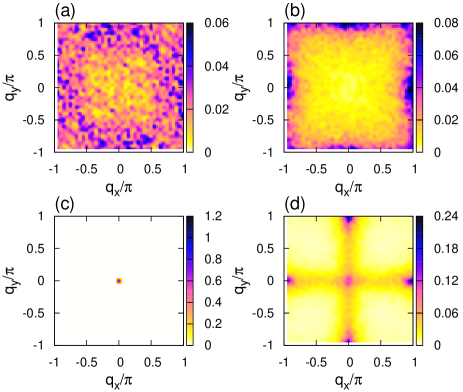
Figure 1: Momentum distribution of the dipolar (top row) and quadrupolar (bottom row) magnetic structure factors at $K_{2}=-1$ (in (a) and (c)) and $K_{2}=1.5$ (in (b) and (d)), respectively. Here, $J_{1}=J_{2}=1$, $J_{3}=K_{3}=0$, and $K_{1}=-1$. The calculations are done on a 40$\times$40 lattice at $T/|K_{1}|$=0.01 with up to $10^{5}$ Monte Carlo steps. In (d), besides the leading AFQ correlations at $(\pi,0)$ and $(0,\pi)$, subleading FQ correlations are observed at finite temperatures; as the temperature is lowered, the former is enhanced whereas the latter is is diminished.

Low-temperature phase diagram of the classical spin model.  We first study the model in Eq. (1) for classical spins. For simplicity, we discuss the case $K_{3}=0$. We have calculated the dipolar and quadrupolar magnetic structure factors via Monte Carlo simulations using the standard Metropolis algorithm.MCBook Representative results for the structure factor data are shown in Fig. 1, for $J_{3}=0$ and $J_{1}=J_{2}$. The two cases, corresponding to different values of $K_{2}$, show, respectively, dominant ferroquadrupolar (FQ) and $(\pi,0)$ AFQ correlations, for the finite-size systems studied and at a very low temperature $T/|K_{1}|=0.01$.

Overall, as shown in Fig. 2(a), we find that there are large regimes in the phase diagram in which the FQ and $(\pi,0)$ AFQ moments are almost ordered, while the dipolar moments coexisting with the FQ/AFQ moments are very weakly correlated. Hence in these regimes, the dominant low-temperature order is the FQ/AFQ one. In between these, there is a regime in which the dominant correlation occurs in the $(\pi,0)$ AFM channel.

Similar results for the case of $J_{1}=0$ and $J_{2}=J_{3}$ are shown in Fig. 2(b). A large regime with dominating FQ or $(\pi,0)$ AFQ correlations is also found. The difference from the case of $J_{3}=0$ and $J_{1}=J_{2}$ occurs in the regime with dominant AFM correlations, for which the wavevector is now $(\pm\pi/2,\pm\pi/2)$ as relevant to the FeTe compound.

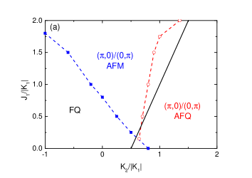
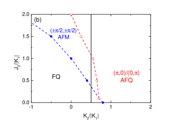
Figure 2: Low-temperature phase diagrams of the classical bilinear-biquadratic Heisenberg model at (a): $J_{1}=J_{2}$, $J_{3}=K_{3}=0$ and (b): $J_{1}=K_{3}=0$, $J_{2}=J_{3}$. Both are shown at $T/|K_{1}|=0.01$. Dashed lines show finite-temperature crossovers between different orders. The dominant order in each regime is labeled. In each case, the solid line shows the mean-field phase boundary at $T=0$.

For 2D systems, thermal fluctuations will ultimately (in the thermodynamic limit) destroy any order that breaks a continuous global symmetry at any nonzero temperature MERMIN-WAGNER . The dashed lines in Fig. 2 therefore mark crossovers between regimes with different dominant correlations. At $T=0$, on the other hand, genuine FQ/AFQ can occur in our model on the square lattice. We have therefore also analyzed the mean-field phase diagrams at $T=0$. The resulting phase boundary is shown in each case as a solid line in Fig. 2. The results are compatible with the crossovers identified at low but nonzero temperatures. For the case of $J_{3}=0$ and $J_{1}=J_{2}$, shown in Fig. 2(a), the phase on the left of the solid line has a mixture of an AFM phase ordered at $\mathbf{q}=(\pi,0)/(0,\pi)$ and a FQ phase. The phase on the right of the solid line has an AFQ phase ordered at $\mathbf{q}=(\pi,0)/(0,\pi)$. Note that in the classical limit, the spins are treated as O(3) vectors, and should always be ordered at zero temperature. We find that in the AFQ phase, the spins can be ordered at a wavevector $(q,\pi)/(\pi,q)$ for arbitrary $q$, with an infinite degeneracy.SM Such a frustration would likely stabilize a purely AFQ ground state when quantum fluctuations are taken into account (see below). For the case of $J_{1}=0$ and $J_{2}=J_{3}$, shown in Fig. 2(b), the mean-field result also yields FQ or $(\pi,0)$ AFQ, respectively, to the left or right of the solid line. However, the wave vector for the AFM orders that mix, respectively, with the FQ and $(\pi,0)$ AFQ order has become $(\pm\pi/2,\pm\pi/2)$.SM

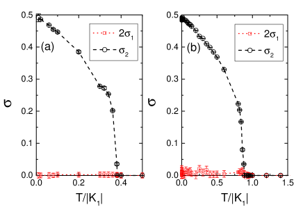
Figure 3: Temperature dependence of the Ising-nematic order parameters $\sigma_{1}$ and $\sigma_{2}$ at (a) $J_{1}=J_{2}=J_{3}=0$, $K_{1}=-1$, and $K_{2}=1$ and (b) $J_{1}=0$, $J_{2}=J_{3}=0.5$, $K_{1}=-1$, and $K_{2}=2$. In both cases the dominant part of the Ising-nematic order is $\sigma_{2}$, which is associated with the AFQ order.

Similar to the $(\pi,0)$ AFM state, the $(\pi,0)$ AFQ phase breaks the lattice $C_{4}$ rotational symmetry. An accompanying Ising-nematic transition is to be expected, and should develop at nonzero temperatures even in two dimensions. We define the general Ising-nematic operators as follows:

$$\sigma_{n}=(\mathbf{S}_{i}\cdot\mathbf{S}_{i+\hat{x}})^{n}-(\mathbf{S}_{i}\cdot\mathbf{S}_{i+\hat{y}})^{n},$$ (3)

where $n=1,2$. We also introduce the quadrupolar $\mathbf{Q}_{A/B}$ to be the linear superposition of $\mathbf{Q}(\pi,0)/(0,\pi)$, with the ratios of their coefficients to be $\pm 1$ respectively. From Eq. (2), we see that for quantum spins, the Ising-nematic order associated with $\mathbf{Q}$ should be seen in both $\sigma_{1}$ and $\sigma_{2}$. For classical spins, since $\mathbf{Q}_{i}\cdot\mathbf{Q}_{j}=2(\mathbf{S}_{i}\cdot\mathbf{S}_{j})^{2}-\frac{2}{3}\mathbf{S}_{i}^{2}\mathbf{S}_{j}^{2}$, only $\sigma_{2}$ will manifest $\mathbf{Q}_{A}\cdot\mathbf{Q}_{B}$. This allows us to determine the origin of the Ising-nematic order in the AFQ+AFM phase. As shown in Fig. 3(a), for the $K_{1}-K_{2}$ model, $\sigma_{2}$ is ordered at $T_{\sigma}/|K_{1}|\approx 0.38$ but $\sigma_{1}\approx 0$ for any $T>0$. Likewise from Fig. 3(b), in the case $J_{1}=0$ and $J_{2}=J_{3}$, the dominant Ising nematic order parameter is $\sigma_{2}$ for $T<T_{\sigma}\approx 0.9$, and $\sigma_{1}$ never becomes substantial down to the lowest temperature $T=10^{-4}$ accessible to our numerical simulation. These indicate that the Ising-nematic order in the AFQ+AFM phase is associated with the anisotropic spin quadrupolar fluctuations.

The quantum spin models.  The AFQ phase and the associated Ising-nematic transition are features of the generalized $J-K$ model for both classical and quantum spins. To consider the effect of quantum fluctuations, we consider the case of $S=1$. We study its ground-state properties via a semiclassical variational approach by using an SU(3) representation LauchliMilaPenc06 , and identify parameter regimes that stabilize the AFQ phase. We further study the spin excitations in the AFQ phase with the ordering wavevector $\mathbf{q}_{A}=(\pi,0)$ using a flavor-wave theory.SM Because the AFQ order breaks the continuous spin-rotational invariance, the Goldstone modes will have a nonzero dipolar matrix element LauchliMilaPenc06 ; Tsunetsugu06 . To explicitly demonstrate this, we calculate the dynamical spin dipolar structure factor $S^{xx}_{D}(\mathbf{q},\omega)$ near $\mathbf{q}_{A}$, which is shown in Fig. 4. Therefore, the development of the AFQ order is accompanied by a sharp rise in the dynamical spin dipolar correlations centered around the wavevector $(\pi,0)$ (and symmetry-related wave vectors).

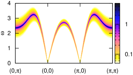
Figure 4: Calculated spin excitation spectrum in the $(\pi,0)$ AFQ phase of the quantum $S=1$ model. We have taken $J_{1}=J_{2}=0.25$, $J_{3}=0$, $K_{2}=0.5$, and $K_{3}=-0.3$. The color codes the dynamical spin dipolar structure factor, $\sqrt{S^{xx}_{D}(\mathbf{q},\omega)}$.

Coupling to itinerant fermions and interaction between layers.  One additional effect of the quantum fluctuations is that it can suppress the weak AFM order when the dominant order is AFQ. We discuss one source of such an effect, which is the coupling of the order parameters to the coherent itinerant fermions. The effect of coupling to the itinerant fermions can be treated as in Ref. JDai09 within an effective Ginzburg-Landau action, and is briefly discussed in the Supplemental Material SM . When only the $(\pi,0)$ AFM order and the Ising-nematic order are present, the coupling to the itinerant fermions will suppress the AFM and Ising-nematic order concurrently JWu14 . However, when the dominant order is AFQ, the coupling to the itinerant fermions can suppress the AFM order while retaining the stronger AFQ order and the associated Ising-nematic order.

When interlayer bilinear-biquadratic couplings are taken into account, a phase with a pure AFQ order can be stabilized at finite temperature. We can then discuss the evolution of the Ising-nematic transition as a function of the $J_{2}/K_{2}$ ratio. Consider the case when a dominating $J_{2}$ stabilizes a $(\pi,0)$ AFM order, which is accompanied by the Ising-nematic order parameter $\sigma_{1}$. For sufficiently large $K_{2}$, the AFQ order becomes the dominant order, and the Ising-nematic order is predominantly given by $\sigma_{2}$. The schematic evolution between the two limits is illustrated in Fig. 5. We have illustrated the case with the quantum fluctuations having suppressed the weaker order.

We stress that, such an evolution of the Ising-nematic transition already occurs in the purely 2D model. Results from explicit calculations on the evolution of the transition temperature $T_{\sigma}$ are shown in the Supplemental Material.SM In the case of the Ising-nematic transition associated with a $(\pi,0)$ AFM order, the interlayer couplings give rise to a nonzero $T_{AFM}\leq T_{\sigma}$ (Refs. Fang08, ; Xu08, ; JDai09, ). Similarly, when the dominant order is a $(\pi,0)$ AFQ order, such couplings lead to a nonzero $T_{AFQ}\leq T_{\sigma}$.

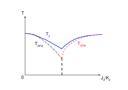
Figure 5: Skecthed phase diagram in terms of $T$ and $J_{2}/K_{2}$. The dominant order may be either AFQ or AFM. The thinner dashed lines show the associated ordering temperautures $T_{AFQ}$ and $T_{AFM}$. A first-order transition (thicker dashed line) takes place at an intermediate $J_{2}/K_{2}$ coupling when the two transitions meet. The Ising-nematic transition (solid line) takes place at $T_{\sigma}$. There can be either a first-order Ising-nematic and AFM(AFQ) transition at $T_{\sigma}=T_{AFM/AFQ}$, or two separate transitions.

Implications for FeSe. General considerations suggest that the cases of spin 1 or spin 2 are pertinent to the iron-based materials SiAbrahams08 . Judging from the measured total spin spectral weight  PCDai_review12 , the spin 1 case would be closer to the iron pnictides while the spin 2 case would be more appropriate for the iron chalcogenides.

Accordingly, it is natural to propose that the normal state of FeSe realizes the phase whose ground state has the $(\pi,0)$ AFQ order accompanied by the Ising-nematic order. In this picture, the structural transition at $T_{s}\sim 90$ K corresponds to the concurrent Ising-nematic and AFQ transition, as illustrated in Fig. 5. This picture explains why the structural phase transition is not accompanied by any static AFM order. At the same time, as soon as the AFQ order is developed, its Goldstone modes will contribute towards low-energy dipolar magnetic fluctuations. This is consistent with the onset of low-energy spin fluctuations observed in the NMR measurements Bohmer14 ; Baek14 . It will clearly be important to explore such spin fluctuations using inelastic neutron scattering measurements. A quantitative comparison between the measured and calculated spin excitation spectra would allow estimates of the coupling constants $J_{n}$ and $K_{n}$. The Goldstone modes may also be probed by magnetoresistance, and unusual features in this property have recently been reported Rossler14 . Finally, the Ising-nematic order is linearly coupled not only to the structural anisotropy, but also to the orbital order. Similarly as for the iron pnictides Yi11 , this would result in, for instance, the lifting of the d_xz/d_yz orbital degeneracy at the structural phase transition Nakayama14 ; Shimojima14 ; Coldea14 .

The phase diagrams given in Fig. 2 show that the AFQ region can be tuned to an AFM region. The nature of the AFM phase depends on the bilinear couplings. For a range of bilinear couplings, the nearby AFM phase has the ordering wavevector $(\pi/2,\pi/2)$. This provides a means to connect the magnetism of FeSe and FeTe Bao ; Li , which is of considerable interest to the on-going experimental efforts in studying the magnetism of the Se-doped FeTe series Tranquada14 . It also makes it natural to understand the development of magnetic order that seems to occur when FeSe is placed under a pressure on the order of $1$ GPa  Bendele10 ; Bendele12 ; Imai09 . Finally, we note that our results will serve as the basis to shed new light on the nematic correlations in the superconducting state Song11 ; HungWu12 ; Chowdhury11 .

Broader context.  It is widely believed that understanding the magnetism in the iron chalcogenide FeTe, where the ordering wavvector $(\pi/2,\pi/2)$ has no connection with any Fermi-surface-nesting features Bao ; Li , requires a local-moment picture. The proposal advanced here not only provides an understanding of the emerging puzzle on the magnetism in FeSe, but also achieves a level of commonality in the underlying microscopic interactions across these iron chalcogenides. Furthermore, the connection between the AFQ order and the $(\pi,0)$ AFM order suggests that the local-moment physics, augmented by a coupling to the coherent itinerant fermions near the Fermi energy, places the magnetism of a wide range of iron-based superconductors in a unified framework. Since local-moment physics in bad metals reflects a proximity to correlation-induced electron localization, this unified perspective also signifies the importance of electron correlations SiAbrahams08 ; Yin ; KSeo ; Moreo ; Lv ; Yu2013 to the iron-based superconductors.

Conclusions. To summarize, we have studied a generalized Heisenberg model with frustrated bilinear-biquadratic interactions on a square lattice and find that the zero-temperature phase diagram stabilizes an antiferroquadrupolar order. The anisotropic spin quadrupolar fluctuations give rise to a finite-temperature Ising-nematic transition. We propose that the structural phase transition in FeSe corresponds to this Ising-nematic transition and is accompanied by an antiferroquadrupolar ordering. We suggest that inelastic neutron scattering experiments be carried out to explore the proposed Goldstone modes associated with the antiferroquadrupolar order. Our results provide a natural understanding for an emerging puzzle on FeSe. More generally, the extended phase diagrams advanced here considerably broaden the perspective on the magnetism and electron correlations of the iron-based superconductors.

Note added.  Recently, a study appeared that also emphasized the local-moment-based magnetic physics for FeSe, but invoked a different mechanism based on a possible paramagnetic Ising-nematic ground state caused by $J_{1}$-$J_{2}$ frustration FWang15 . A distinction of the mechanism advanced here is that the AFQ order yields Goldstone modes and therefore causes the onset of low-energy dipolar magnetic fluctuations. In addition, results from inelastic neutron scattering experiments in FeSe have appeared Rahn15 ; WangZhao15 , which verify the $(\pi,0)$ magnetic excitations expected from our theoretical proposal.

We would like to acknowledge an early conversation with C. Meingast, A. Böhmer and F. Hardy, which stimulated our interest in this problem, and useful discussions with E. Abrahams, B. Büchner, A. Coldea, P. Dai, D.-H. Lee, and A. H. Nevidomskyy. This work was supported in part by NSF Grant No. DMR-1309531, Robert A. Welch Foundation Grant No. C-1411 and the Alexander von Humboldt Foundation. R.Y. was partially supported by National Science Foundation of China Grant No. 11374361, and the Fundamental Research Funds for the Central Universities and the Research Funds of Renmin University of China. Both of us acknowledge the support provided in part by NSF Grant No. NSF PHY11-25915 at KITP, UCSB, for our participation in the Fall 2014 program on “Magnetism, Bad Metals and Superconductivity: Iron Pnictides and Beyond.” Q.S.  also acknowledges the hospitality of the the Karlsruhe Institute of Technology, the Aspen Center for Physics (NSF Grant No. 1066293), and the Institute of Physics of the Chinese Academy of Sciences.

I SUPPLEMENTARY MATERIAL – Antiferroquadrupolar and Ising-nematic orders of a frustrated bilinear-biquadratic Heisenberg model and implications for the magnetism of FeSe

I.1 The ground-state spin configurations in the classical spin model

Exactly at $T=0$, the classical $O(3)$ spins are always ordered. Therefore, the AFQ order is accompanied by magnetic dipolar orders. Because the $(\pi,0)$ AFQ order doubles the unit cell, the structure factor $\mathcal{S}_{D}(\mathbf{q})$ of the compatible magnetic dipolar order must show a two-$q$ structure as the consequence of Brillion zone folding, i.e., $\mathcal{S}_{D}(\mathbf{q})=\mathcal{S}_{D}(\mathbf{q}+\mathbf{q}_{A})$ where $\mathbf{q}_{A}=(\pi,0)$. The ordering wavevector $\mathbf{q}$ depends on model parameters.

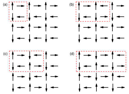
Figure S1: Four among the infinitely degenerate ground-state spin patterns in the case of $J_{3}=0$ and $J_{1}=J_{2}$. In each case, the dashed box shows the magnetic unit cell. The corresponding ordering wavevectors are as follows: $\mathbf{q}=(0,\pi)$ and $(\pi,\pi)$ in (a); $\mathbf{q}=(\pm\pi/2,\pi)$ in (b) and (c); $\mathbf{q}=(2\pi/3,\pi)$ and $(-\pi/3,\pi)$ in (d).

We find that in the $(\pi,0)/(0,\pi)$ AFQ ground state the spins are ordered at a wavevector $(q,\pi)/(\pi,q)$ with infinite degeneracies for $J_{3}=0$. Assuming a $(\pi,0)$ AFQ order, the spin variable at site $i$ is $\mathbf{S}_{i}=\xi(i_{x})[\hat{e}_{x}\gamma(i_{x})+\hat{e}_{y}(1-\gamma(i_{x}))]\gamma(i_{y})$, where $i_{x}$ and $i_{y}$ are coordinates of site $i$, $\gamma(i_{x(y)})=(1+(-1)^{i_{x(y)}})/2$, and $\xi(i_{x})=\pm 1$ is a random variable defined on each column of the lattice. The randomness in the real-space spin configuration leads to infinite number of degenerate ground-state spin patterns. Transforming to the momentum space, they correspond to ordering wavevector at $(q,\pi)$ (and $(q+\pi,\pi)$) with $q$ an arbitrary number. Some of the degenerate spin patterns are shown in Fig. S1.

As for the case of $J_{1}=0$ and $J_{2}=J_{3}$, in the AFQ phase, we still find 16-fold degenerate ground-state spin patterns at ordering wavevectors $(\pm\pi/2,\pm\pi/2)$. Some of the spin patterns are shown in Fig. S2. In both cases, the large number of degenerate classical spin ground states helps to stabilize an AFQ order without a magnetic dipolar one when the quantum fluctuations are taken into account.

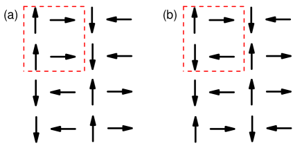
Figure S2: Two out of the $16$ degenerate ground-state spin patterns in the case of $J_{1}=0$ and $J_{2}=J_{3}$. In each case, the spin pattern can be obtained by repeatedly aligning the spins in the dashed box in a staggered way. In both cases, the ordering wavevectors are $\mathbf{q}=(\pm\pi/2,\pm\pi/2)$ .

Another interesting observation is that at $T=0$, the dominant $(\pi,0)$ AFQ order of $Q^{x^{2}-y^{2}}$ coexists with a subleading FQ order of $Q^{r^{2}-3z^{2}}$. This can be checked using the ground-state spin configurations in Figs. S1 and S2, which gives $Q^{r^{2}-3z^{2}}_{i}=1/\sqrt{3}$ at each site and $Q^{x^{2}-y^{2}}=\pm 1$.

I.2 Spin excitations and Goldstone modes in the quantum $S=1$ model

For the case of quantum spin $S=1$, the model defined in Eq. (1) of the main text can be studied by an SU(3) Schwinger boson approach.SMLauchliMilaPenc06 At each site, let $|-1\rangle$, $|0\rangle$, and $|1\rangle$ be the three eigenstates of the spin operator $S^{z}$. We can define a time-reversal invariant basis of the SU(3) representation:

$$|x\rangle =\frac{i}{\sqrt{2}}\left(|1\rangle-|-1\rangle\right),$$

$$|y\rangle =\frac{1}{\sqrt{2}}\left(|1\rangle+|-1\rangle\right),$$ (S1)

$$|z\rangle =-i|0\rangle.$$

Within this representation, we can then define three Schwinger bosons associated with the above three states, $b^{\dagger}_{\alpha}|\not{0}\rangle=|\alpha\rangle$, where $\alpha=x$, $y$, $z$, and $|\not{0}\rangle$ is the null state of the Schwinger bosons. The three bosons satisfy a local constraint at each site:

$$\sum_{\alpha}b^{\dagger}_{i\alpha}b_{i\alpha}=1.$$ (S2)

The spin dipolar and quadrupolar operators can be written in terms of the Schwinger boson bilinears as

$$S^{\alpha}_{i} =-i\epsilon_{\alpha\beta\gamma}(b^{\dagger}_{i\beta}b_{i\gamma}-b^{\dagger}_{i\gamma}b_{i\beta}),$$ (S3)

$$Q^{\alpha\beta}_{i} =-(b^{\dagger}_{i\alpha}b_{i\beta}+b^{\dagger}_{i\beta}b_{i\alpha}),$$

$$Q^{x^{2}-y^{2}}_{i} =-(b^{\dagger}_{ix}b_{ix}-b^{\dagger}_{iy}b_{iy}),$$ (S4)

$$Q^{r^{2}-3z^{2}}_{i} =\frac{1}{\sqrt{3}}(2b^{\dagger}_{iz}b_{iz}-b^{\dagger}_{ix}b_{ix}-b^{\dagger}_{iy}b_{iy}),$$

where $\alpha$, $\beta$, and $\gamma$ run over $x$, $y$, and $z$, and $\epsilon_{\alpha\beta\gamma}$ is the Levi-Civita symbol. The Hamiltonian is then rewritten as

$$H =\frac{1}{2}\sum_{i,\delta_{n},\alpha,\beta}\left\{J_{n}b^{\dagger}_{i\alpha}b_{j\alpha}b^{\dagger}_{j\beta}b_{i\beta}+(K_{n}-J_{n})b^{\dagger}_{i\alpha}b^{\dagger}_{j\alpha}b_{j\beta}b_{i\beta}\right\},$$

where $j=i+\delta_{n}$, and $\delta_{n}$ (with $n=1$, $2$, $3$) connects site $i$ and its $n$’s nearest neighbor sites.

We assume the following ground state at the mean level: $|\psi\rangle=\Pi_{i}|\psi_{i}\rangle=\Pi_{i}\sum_{\alpha}f_{i\alpha}b^{\dagger}_{i\alpha}|\not{0}\rangle$, where the coefficients satisfy $\sum_{\alpha}|f_{i\alpha}|^{2}=1$. The $(\pi,0)$ AFQ order can be obtained by requiring condensation of $b_{x}$ and $b_{y}$ bosons at sites in odd and even columns, respectively. Correspondingly, the mean-field ground-state wave function at site $i$ is $|\psi_{i}\rangle=|x\rangle_{i}$ if the $x$ coordinate of site $i$ ($i_{x}$) is odd, and $|\psi_{i}\rangle=|y\rangle_{i}$ if $i_{x}$ is even. One could check that this wave function is indeed associated to an AFQ order at wavevector $\mathbf{q}_{A}=(\pi,0)$ since $\langle\psi_{i}|Q^{x^{2}-y^{2}}|\psi_{i}\rangle=e^{\mathbf{q}_{A}\cdot\mathbf{r}_{i}}=\pm 1$.

We study the spin excitations in the AFQ phase by using a flavor-wave theory. We first perform a local rotation in the spin space,

$$\left(\begin{tabular}[]{c}$d_{ix}$\\ $d_{iy}$\\ $d_{iz}$\end{tabular}\right) =\left(\begin{tabular}[]{ccc}$\cos\theta_{i}$&$\sin\theta_{i}$&$0$\\ $-\sin\theta_{i}$&$\cos\theta_{i}$&$0$\\ $0$&$0$&$1$\end{tabular}\right)\left(\begin{tabular}[]{c}$b_{ix}$\\ $b_{iy}$\\ $b_{iz}$\end{tabular}\right),$$ (S6)

such that in the rotated basis, only one flavor of bosons, $d_{ix}$, condenses. In the $(\pi,0)$ AFQ phase, this corresponds to taking $\theta_{i}=0$ if $i_{x}$ is odd and $\theta_{i}=\pi/2$ if $i_{x}$ is even. Using the constraint in this rotated basis, $\sum_{\alpha}d^{\dagger}_{i\alpha}d_{i\alpha}=1$, we obtain

$$d_{ix} \rightarrow\sqrt{1-d^{\dagger}_{iy}d_{iy}-d^{\dagger}_{iz}d_{iz}}$$

$$\approx 1-\frac{1}{2}(d^{\dagger}_{iy}d_{iy}+d^{\dagger}_{iz}d_{iz}).$$ (S7)

Using Eq. (I.2), we can expand the Hamiltonian in Eq. (I.2) in terms of the magnon operators $d_{iy}$, $d_{iz}$, and their Hermitian conjugates. We then truncate the expanded Hamiltonian to keep up to the quadratic terms of $d_{iy}$, $d_{iz}$, and their Hermitian conjugates. Given that the ground state is the AFQ state, the linear terms in $d_{iy}$, $d_{iz}$ automatically cancel out, and we arrive at, up to a constant energy, a quadratic Hamiltonian. After Fourier transforming it to the momentum space, this quadratic Hamiltonian reads,

$$H\approx\sum_{k,\alpha=y,z} A_{k\alpha}(d^{\dagger}_{k\alpha}d_{k\alpha}+d_{-k\alpha}d^{\dagger}_{-k\alpha})$$

$$+ B_{k\alpha}(d^{\dagger}_{k\alpha}d^{\dagger}_{-k\alpha}+d_{k\alpha}d_{-k\alpha}).$$ (S8)

Here $k$ runs over the unfolded Brilluion zone (BZ), and

$$A_{ky} =J_{1}(\cos k_{x}+\cos k_{y})-K_{1}\cos k_{x}$$

$$-2(K_{2}-J_{2})\cos k_{x}\cos k_{y}+J_{3}(\cos 2k_{x}+\cos 2k_{y})$$

$$+2K_{2}-2K_{3},$$ (S9)

$$B_{ky} =K_{1}\cos k_{y}-J_{1}(\cos k_{x}+\cos k_{y})-2J_{2}\cos k_{x}\cos k_{y}$$

$$+(K_{3}-J_{3})(\cos 2k_{x}+\cos 2k_{y}),$$ (S10)

$$A_{kz} =J_{1}\cos k_{y}+J_{3}(\cos 2k_{x}+\cos 2k_{y})-K_{1}-2K_{3},$$ (S11)

$$B_{kz} =(K_{1}-J_{1})\cos k_{y}+(K_{3}-J_{3})(\cos 2k_{x}+\cos 2k_{y}).$$ (S12)

The Hamiltonian in Eq. (I.2) can be diagonalized via a Bogoliubov transformation

$$d_{ky(z)} =u_{ky(z)}\gamma_{ky(z)}-v_{ky(z)}\gamma_{ky(z)}^{\dagger},$$ (S13)

and

$$H \approx\sum_{k,\alpha=y,z}\epsilon_{k\alpha}(\gamma^{\dagger}_{k\alpha}\gamma_{k\alpha}+\gamma_{-k\alpha}\gamma_{-k\alpha}^{\dagger}),$$ (S14)

where the magnon dispersion

$$\epsilon_{k\alpha} =\sqrt{A^{2}_{k\alpha}-B^{2}_{k\alpha}},$$ (S15)

and

$$u_{k\alpha} =\frac{1}{2}\left(\frac{A_{k\alpha}}{\sqrt{A^{2}_{k\alpha}-B^{2}_{k\alpha}}}+1\right),$$

$$v_{k\alpha} =\frac{1}{2}\left(\frac{A_{k\alpha}}{\sqrt{A^{2}_{k\alpha}-B^{2}_{k\alpha}}}-1\right).$$ (S16)

The parameter regime where the $(\pi,0)$ AFQ phase is stable is obtained by requiring $A_{k\alpha}\geqslant 0$ and $A^{2}_{k\alpha}-B^{2}_{k\alpha}\geqslant 0$ at every $k$ in the entire BZ and for both $\alpha=y,z$, and can be determined numerically.

The dynamical spin dipolar and quadrupolar structure factors $S^{\mu\mu}_{Q}(\mathbf{q},\omega)$ and $S^{\alpha\alpha}_{D}(\mathbf{q},\omega)$ can be calculated within the diagonalized representation. In gerneral,

$$S^{\mu\mu}_{Q}(\mathbf{q},\omega) =\sum_{m}|\langle g|Q^{\mu}_{\mathbf{q}}|m\rangle|^{2}\delta(\omega-(E_{m}-E_{g})),$$ (S17)

$$S^{\alpha\alpha}_{D}(\mathbf{q},\omega) =\sum_{m}|\langle g|S^{\alpha}_{\mathbf{q}}|m\rangle|^{2}\delta(\omega-(E_{m}-E_{g})).$$ (S18)

Here, $|g\rangle$ and $|m\rangle$ refer to the ground state (with eigenenergy $E_{g}$) and the $m$’s excited state (with eigenenergy $E_{m}$) in the flavor-wave theory.

$$Q^{\mu}_{\mathbf{q}}=\frac{1}{\sqrt{N}}\sum_{i}e^{i\mathbf{q}\cdot\mathbf{r}_{i}}Q^{\mu}_{i},$$ (S19)

$$S^{\alpha}_{\mathbf{q}}=\frac{1}{\sqrt{N}}\sum_{i}e^{i\mathbf{q}\cdot\mathbf{r}_{i}}S^{\alpha}_{i},$$ (S20)

where $N$ is the number of spins of the system, and $Q^{\mu}_{i}$ and $S^{\alpha}_{i}$ are expressed in terms of Schwinger bosons using Eqs. (S3) and  (S4). For example, for $\mu=x^{2}-y^{2}$,

$$Q^{x^{2}-y^{2}}_{\mathbf{q}} =\sqrt{N}\delta_{\mathbf{q},\mathbf{q}_{A}}-\frac{2}{\sqrt{N}}\sum_{k}d^{\dagger}_{ky}d_{k+\mathbf{q}+\mathbf{q}_{A},y}$$

$$-\frac{1}{\sqrt{N}}\sum_{k}d^{\dagger}_{kz}d_{k+\mathbf{q}+\mathbf{q}_{A},z}.$$ (S21)

This leads to $S^{\mu\mu}_{Q}(\mathbf{q},\omega)=N\delta_{\mathbf{q},\mathbf{q}_{A}}\delta(\omega)$ up to the one-magnon contribution, which confirms the AFQ order at $\mathbf{q}_{A}=(\pi,0)$.

The one-magnon contribution to the spin dipolar correlation function is also non-zero. We find that the transverse dynamical structure factor

$$S^{xx}_{D}(\mathbf{q},\omega)=S^{yy}_{D}(\mathbf{q},\omega) =\frac{1}{2}\sqrt{\frac{A_{\mathbf{q}z}+B_{\mathbf{q}z}}{A_{\mathbf{q}z}-B_{\mathbf{q}z}}}\delta(\omega-\epsilon_{\mathbf{q}z})$$ (S22)

From Eqs. (S11),(S12), and (S15), we find a Goldstone mode near $\mathbf{q}_{A}=(\pi,0)$. For $\mathbf{q}=\mathbf{q}_{A}+(dq_{x},dq_{y})$,

$$\epsilon_{\mathbf{q}z} \approx\sqrt{v_{x}^{2}dq_{x}^{2}+v_{y}^{2}dq_{y}^{2}},$$ (S23)

with anisotropic velocities

$$v_{x} =2\sqrt{K_{3}\eta},$$

$$v_{y} =\sqrt{(K_{1}+4K_{3})\eta},$$ (S24)

where $\eta=K_{1}+2K_{3}-J_{1}-2J_{3}$. The Goldstone mode near $\mathbf{q}_{A}$ is also seen in the dynamical spin dipolar structure factor:

$$S^{xx}_{D}(\mathbf{q}\to\mathbf{q}_{A},\omega)\approx\frac{\omega}{2\eta}\delta(\omega-\epsilon_{\mathbf{q}z}).$$ (S25)

Note that the static dipolar structure factor $S^{xx}_{D}(\mathbf{q}_{A})=0$, because of the absence of long-range magnetic dipolar order in the AFQ phase. But the Goldstone modes associated with the broken spin rotational symmetry can be observed from the dynamical spin dipolar structure factor. A representative plot of $S^{xx}_{D}(\mathbf{q},\omega)$ showing the Goldstone modes is displayed in Fig. 4 of the main text.

I.3 Quantum fluctuations and coupling to itinerant fermions. 

The field theory that describes the two coupled order parameters $\mathbf{Q}_{A}$ and $\mathbf{Q}_{B}$ will be similar to that of the $(\pi,0)$ AFM order of the $J_{1}-J_{2}$ Heisenberg model. The effect of coupling to the itinerant fermions can be treated as in Ref. SMJDai09 within an effective Ginzburg-Landau action:

$${\cal S}({\bf Q}_{A},{\bf Q}_{B}) =\int d\{\bf q\}\int d\{\omega\}[{\cal S}_{2}+{\cal S}_{4}+\dots],$$

$${\cal S}_{2}({\bf q},\omega) =r(\omega,\mathbf{q})[|{\bf Q}_{A}({\bf q},\omega)|^{2}+|{\bf Q}_{B}({\bf q},\omega)|^{2}]$$

$$+v(q_{x}^{2}-q_{y}^{2})[{\bf Q}_{A}({\bf q},\omega)\cdot{\bf Q}_{B}({-\bf q},-\omega)],$$

$${\cal S}_{4}(\{{\bf q}\},\{\omega\}) =u(|{\bf Q}_{A}|^{4}+|{\bf Q}_{B}|^{4})+u^{\prime}|{\bf Q}_{A}|^{2}\;|{\bf Q}_{B}|\,^{2}$$

$$+{\tilde{u}}|{\bf Q}_{A}\cdot{\bf Q}_{B}|^{2}.$$ (S26)

where $r(\omega,\mathbf{q})=r_{0}+wA+\omega^{2}+\gamma|\omega|+cq^{2}$, $r_{0}<0$ and $A>0$ are constants, $w$ is the coherent quasiparticle spectral weight of itinerant electrons, and $\gamma$ is a Landau-damping coefficient. Note that ${\tilde{u}}<0$, and $\{{\bf q}\},\{\omega\}$ mark the set of four momenta and four frequencies that enter $S_{4}$; the momentum and frequency integrals are understood to each contain a delta function that fixes the sum of the momenta and the sum of the frequencies at zero. A similar form also exists for the AFM orders, $\mathbf{M}_{A}$ and $\mathbf{M}_{B}$  SMJDai09 . The shift of $r$ by $w$ and the damping may lead to the loss of magnetic order in the system SMJDai09 , and stabilize a pure AFQ order. In the absence of the AFQ order, the Ising-nematic order will be concurrently suppressed SMJWu14 . However, when the dominant order is AFQ, one can readily reach the regime where the quantum fluctuations eliminate the weaker AFM order while retaining the stronger AFQ order and the associated Ising-nematic order.

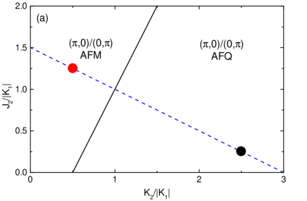
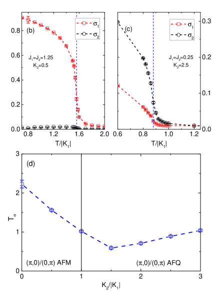
Figure S3: (a): Mean-field ground-state phase diagram of the classical bilinear-biquadratic Heisenberg model at $J_{3}=K_{3}=0$ and $J_{1}=J_{2}$. The blue dashed line shows the trajectory by tuning $J_{2}/K_{2}$, and the red and black dots show two representative points along this trajectory. (b) and (c): Temperature dependence of the Ising-nematic order parameters $\sigma_{1}$ and $\sigma_{2}$ at the two representative points of the phase diagram in panel (a). There is a change of the dominant Ising-nematic order parameter from $\sigma_{1}$ to $\sigma_{2}$ when the ground state varies from the AFM to the AFQ phase. The blue dashed line marks the transition temperature, $T_{\sigma}$, of the Ising-nematic transition. Data shown are based on Monte Carlo simulations on a $40\times 40$ lattice. (d): Evolution of $T_{\sigma}$ with varying $J_{2}/K_{2}$ along the trajectory shown in panel (a). A minimum of $T_{\sigma}$ is located near the phase boundary (black solid line) between the AFM and the AFQ phase, which is consistent with the proposal made in the main text, as illustrated in Fig. 5 of the main text.

I.4 The evolution of the Ising-nematic order parameter and transition temperature as a function of $J_{2}/K_{2}$

Here we study how the dominant Ising-nematic order parameter and the associated transition temperature, $T_{\sigma}$, change with varying the $J_{2}/K_{2}$ ratio in the 2D classical bilinear-biquadratic Heisenberg model. The calculations are done via classical Monte Carlo simulations using Metropolis sampling with up to $80\times 80$ lattices and $10^{5}$ Monte Carlo steps.

We tune the $J_{2}/K_{2}$ ratio by going along the blue dashed trajectory in the phase diagram shown in Fig. S3(a). As discussed in the main text, with increasing $K_{2}$, the ground state of the system changes from the $(\pi,0)/(0,\pi)$ AFM to the $(\pi,0)/(0,\pi)$ AFQ state. We have tracked the evolution of the Ising-nematic order parameters $\sigma_{1}$ and $\sigma_{2}$, and find that the change of the ground state is reflected in the variation of the Ising-nematic order parameters: the dominant Ising-nematic order parameter changes from $\sigma_{1}$ in the AFM phase to $\sigma_{2}$ in the AFQ phase, as clearly shown in Fig. S3(b) and (c). We have also determined the transition temperature $T_{\sigma}$ from our numerical results. $T_{\sigma}$ first decreases then increases with increasing $K_{2}$ along the trajectory, showing a remarkable minimum near the phase boundary between the AFM and AFQ phases (Fig. S3(d)). This minimum indicates enhanced fluctuations around the Ising-nematic order due to the competition between the AFM and AFQ orders. Our results on the evolution of the dominant Ising-nematic order parameter and $T_{\sigma}$ with $J_{2}/K_{2}$ are fully consistent with the general picture proposed in Fig. 5 of the main test. When an interlayer coupling is turned on, we expect similar results for the Ising-nematic order, because the change of the dominant Ising-nematic order parameter and the evolution of $T_{\sigma}$ reflect the competition between the underlying AFM and AFQ ground states. In this case, in the dominating AFM regime, it is well known that a nonzero transition temperature develops for the AFM order. Similar reasoning applies to the dominating AFQ regime.

References

- (1) P. Dai, J. Hu, and E. Dagotto, Nat. Phys. 8, 709 (2012).
- (2) Q. Si and E. Abrahams, Phys. Rev. Lett. 101, 076401 (2008).
- (3) P. Chandra, P. Coleman, and A. I. Larkin, Phys. Rev. Lett. 64, 88 (1990).
- (4) C. Fang et al., Phys. Rev. B 77, 224509 (2008).
- (5) C. Xu, M. Muller, and S. Sachdev, Phys. Rev. B 78, 020501(R) (2008).
- (6) J. Dai et al., Proc. Natl. Acad. Sci. USA 106, 4118 (2009).
- (7) R. M. Fernandes, A. V. Chubukov, and J. Schmalian, Nat. Phys. 10, 97 (2014).
- (8) S. O. Diallo et al., Phys. Rev. B 81, 214407 (2010).
- (9) L. W. Harriger et al., Phys. Rev. B 84, 054544 (2011).
- (10) R. Yu, Z. Wang, P. Goswami, A. H. Nevidomskyy, Q. Si and E. Abrahams, Phys. Rev. B 86, 085148 (2012).
- (11) A. L.Wysocki, K. D. Belashchenko, and V. P. Antropov, Nat. Phys. 7, 485 (2011); J. P. Hu et al., Phys. Rev. B 85, 144403 (2012); J. K. Glasbrenner et al., Phys. Rev. B 89, 064509 (2014).
- (12) F.-C. Hsu et al., Proc. Natl. Acad. Sci. USA 105, 14262 (2008).
- (13) M. H. Fang et al., Phys. Rev. B 78, 224503 (2008).
- (14) Q.-Y. Wang et al., Chin. Phys. Lett. 29, 037402 (2012).
- (15) J.-F. Ge et al., Nat. Mater. 10, doi: 10.1038/nmat4153.
- (16) J. J. Lee et al., Nature 515, 245 (2014).
- (17) J. He et al., Proc. Natl. Acad. Sci. USA 111, 18501 (2014).
- (18) T. M. McQueen et al., Phys. Rev. Lett. 103, 057002 (2009).
- (19) S. Medvedev et al., Nat. Mater. 8, 630 (2009).
- (20) A. E. Böhmer et al., Phys. Rev. Lett. 114, 027001 (2015).
- (21) S.-H. Baek et al., Nat. Mater. 14, 210 (2015).
- (22) F. Ma, W. Ji, J. Hu, Z.-Y. Lu, and T. Xiang, Phys. Rev. Lett. 102, 177003 (2009).
- (23) P. Fazekas, Lecture Notes on Electron Correlation and Magnetism (World Scientific, Singapore 1999).
- (24) D. P. Landau and K. Binder, A Guide to Monte Carlo Simulations in Statistical Physics (Cambridge University Press, New York, 2000).
- (25) N. D. Mermin and H. Wagner, Phys. Rev. Lett. 17 1133 (1966).
- (26) See Supplemental Material for the exact ground state spin configurations in the AFQ phase of the classical spin model, the detailed calculation on the spin excitations of the quantum model, the discussion on the effects of quantum fluctuations associated with the coupling to coherent itinerant fermions, and the evolution of the Ising-nematic transition with tuning .
- (27) A. Läuchli, F. Mila, and K. Penc, Phys. Rev. Lett. 97, 087205 (2006).
- (28) H. Tsunetsugu and M. Arikawa, J. Phys. Soc. Jpn. 75, 083701 (2006).
- (29) J. Wu, Q. Si, and E. Abrahams, arXiv:1406.5136.
- (30) S. Rößler, C. Koz, L. Jiao, U. K. Rößler, F. Steglich, U. Schwarz, and S. Wirth, Phys. Rev. B 92, 060505(R) (2015).
- (31) M. Yi et al., Proc. Natl. Acad. Sci. USA 108, 6878 (2011).
- (32) K. Nakayama et al., Phys. Rev. Lett. 113, 237001 (2014).
- (33) T. Shimojima et al., Phys. Rev. B 90, 121111(R) (2014).
- (34) A. Coldea, talk given at the KITP program on “Magnetism, Bad Metals and Superconductivity: Iron Pnictides and Beyond,” http://online.kitp.ucsb.edu/online/ironic14/coldea/.
- (35) W. Bao et al., Phys. Rev. Lett. 102, 247001 (2009).
- (36) S. Li et al., Phys. Rev. B 79, 054503 (2009).
- (37) J. Tranquada, talk given at the KITP conference on “Strong Correlations and Unconventional Superconductivity”, http://online.kitp.ucsb.edu/online/ironic-c14/tranquada/.
- (38) M. Bendele et al., Phys. Rev. Lett. 104, 087003 (2010).
- (39) M. Bendele et al., Phys. Rev. B 85, 064517 (2012).
- (40) T. Imai et al., Phys. Rev. Lett. 102, 177005 (2009).
- (41) C.-L. Song et al., Science 332, 1410 (2011).
- (42) H.-H. Hung, C.-L. Song, X. Chen, X. Ma, Q.-K. Xue and C. Wu, Phys. Rev. B 85, 104510 (2012).
- (43) D. Chowdhury, E. Berg and S. Sachdev, Phys. Rev. B 84, 205113 (2011).
- (44) Z. P. Yin, K. Haule, and G. Kotliar, Nat. Mater. 10, 932 (2011).
- (45) K. Seo, B. A. Bernevig and J. Hu, Phys. Rev. Lett. 101, 206404 (2008).
- (46) A. Moreo, M. Daghofer, J. A. Riera, and E. Dagotto, Phys. Rev. B 79, 134502 (2009).
- (47) W. Lv, F. Krüger, and P. Phillips, Phys. Rev. B 82, 045125 (2010).
- (48) R. Yu, P. Goswami, Q. Si, P. Nikolic, and J. -X. Zhu, Nat. Commun. 4, 2783 (2013), doi:10.1038/ncomms3783.
- (49) F. Wang, S. Kivelson, and D.-H. Lee, arXiv:1501.00844.
- (50) M. C. Rahn et al., Phys. Rev. B 91, 180501(R) (2015).
- (51) Q. Wang et al., arXiv:1502.07544.

References

- (1) A. Läuchli, F. Mila, and K. Penc, Phys. Rev. Lett. 97, 087205 (2006).
- (2) J. Dai et al., Proc. Natl. Acad. Sci. USA 106, 4118 (2009).
- (3) J. Wu, Q. Si, and E. Abrahams, arXiv:1406.5136.