Gauge invariance and gluon poles for direct photon production

Abstract:

We discuss the hadron tensor of the direct photon production. We study the effects which lead to the soft breaking of factorization by inspection of the corresponding QCD gauge invariance. We emphasize that the special role is played by the contour gauge for gluon fields. We demonstrate that the different prescriptions in the gluonic pole contributions are dictated by the presence of initial or final state interactions in diagrams. Moreover, the different prescriptions that correspond to the initial of final state interactions are needed to ensure the QCD gauge invariance.

1 Introduction

As shown in [1], to ensure the QED gauge invariance of the transverse polarized Drell-Yan (DY) hadron tensor it is a must to include a contribution of the extra diagram which arises from the non-trivial imaginary part of the corresponding twist $3$ function $B^{V}(x_{1},x_{2})$. Previously, however, this function assumed to be a real function (see, for example, [2] where, nevertheless, the needed imaginary part was generated by the specially introduced “propagator” in the hard part of the hadron tensor). As explained in [1], the complex prescription in the representation of $B^{V}$-function can be understood with a help of the contour gauge. Moreover, the account for this extra contribution, owing to the complex $B^{V}$-function, led to the amplification of the hadron tensor by the factor of $2$. Notice that this our finding was independently confirmed in [3] by using of the different approach. The corresponding SSAs, related to the use of the twist $3$ $B^{V}$-function in the DY process, and the role of gluon poles were previously discussed by many groups (see, for example, [4, 5, 6, 7, 8, 9, 10, 11, 12, 13, 14, 15, 16, 17, 18]).

We now present our approach, that was used in [1] and recently developed in [19], to study the effects in the direct photon production (DPP) which lead to the soft breaking of factorization (or the universality breaking) by inspection of the QCD gauge invariance. As in [1], the special role is played by the contour gauge for gluon fields. We, first, demonstrate that the prescriptions for the gluonic poles in the twist $3$ correlators are dictated by the prescriptions in the corresponding hard parts and, second, argue that the different prescriptions in the gluonic poles defined by the initial or final state interactions in the diagrams under consideration (see, [19] for more details). Moreover, the different prescriptions in the representations of $B^{V}$-functions are needed to ensure the QCD gauge invariance. The situation when we have no the universality condition for the corresponding soft function will be treated a soft breaking of factorization.

2 Kinematics

We study the semi-inclusive process where the hadron with the transverse polarization collides with the other unpolarized hadron to produce the direct photon in the final state in:

$$N^{(\uparrow\downarrow)}(p_{1})+N(p_{2})\to\gamma(q)+q(k)+X(P_{X})\,.$$ (1)

For (1) (also for the Drell-Yan process), the gluonic poles manifest [12]. We perform our calculations within a collinear factorization and, therefore, it is convenient (see, e.g., [21]) to fix the dominant light-cone directions as

$$p_{1}=\sqrt{\frac{S}{2}}\,n^{*}\,,\quad p_{2}=\sqrt{\frac{S}{2}}\,n\,,\quad$$

$$n^{*}_{\mu}=(1/\sqrt{2},\,{\bf 0}_{T},\,1/\sqrt{2}),\quad n_{\mu}=(1/\sqrt{2},\,{\bf 0}_{T},\,-1/\sqrt{2})\,.$$ (2)

Accordingly, the quark and gluon momenta $k_{1}$ and $\ell$ lie along the plus dominant direction while the gluon momentum $k_{2}$ – along the minus direction. The final on-shell photon and quark(anti-quark) momenta can be presented as

$$q=y_{B}\,\sqrt{\frac{S}{2}}\,n-\frac{q_{\perp}^{2}}{y_{B}\sqrt{2S}}\,n^{*}+q_{\perp}\,,\quad k=x_{B}\,\sqrt{\frac{S}{2}}\,n^{*}-\frac{k_{\perp}^{2}}{x_{B}\sqrt{2S}}\,n+k_{\perp}\,.$$ (3)

And, the Mandelstam variables for the process and subprocess are defined as

$$S=(p_{1}+p_{2})^{2},\quad T=(p_{1}-q)^{2},\quad U=(q-p_{2})^{2},$$

$$\hat{s}=(x_{1}p_{1}+yp_{2})^{2}=x_{1}yS,\quad\hat{t}=(x_{1}p_{1}-q)^{2}=x_{1}T,\quad\hat{u}=(q-yp_{2})^{2}=yU.$$ (4)

The amplitude (or the hadron tensor) of (1) constructed by the contributions from (i) the leading (LO) diagrams: two diagrams with a radiation of the photon before (${\cal A}^{{\rm LO}}_{1}$) and after (${\cal A}^{{\rm LO}}_{2}$) the quark-gluon vertex with the gluon going to the lower blob, see the right side of Fig. 1; (ii) the next-to-leading order (NLO) diagrams: eight diagrams constructed from the LO diagrams by insertion of all possible radiations of the additional gluon which together with the quark goes to the upper blob, see the left side of Fig. 1. So, we have the hadron tensor related to the corresponding asymmetry:

$$d\sigma^{\uparrow}-d\sigma^{\downarrow}\sim{\cal W}=\sum\limits_{i=1}^{2}\sum\limits_{j=1}^{8}{\cal A}^{{\rm LO}}_{i}\ast{\cal B}^{{\rm NLO}}_{j}\,.$$ (5)

Here, we will mainly discuss the hadron tensor rather than the asymmetry itself. So, the hadron tensor as an interference between the LO and NLO diagrams, ${\cal A}^{{\rm LO}}_{i}\ast{\cal B}^{{\rm NLO}}_{j}$, can be presented by Fig. 1 where the upper blob determines the matrix element of the twist-3 quark-gluon operator while the lower blob – the matrix element of the twist-2 gluon operator related to the unpolarized gluon distribution.

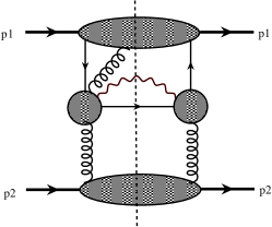
Figure 1: The Feynman diagram describing the hadron tensor of the direct photon production.

3 Factorization procedure

The collinear factorization being our main tool, let us outline the main steps of the factorization procedure. It contains (i) the decomposition of loop integration momenta around the corresponding dominant direction: $k_{i}=x_{i}p+(k_{i}\cdot p)n+k_{T}$ within the certain light cone basis formed by the vectors $p$ and $n$ (in our case, $n^{*}$ and $n$); (ii) the replacement: $d^{4}k_{i}\Longrightarrow d^{4}k_{i}\,dx_{i}\delta(x_{i}-k_{i}\cdot n)$ that introduces the fractions with the appropriated spectral properties; (iii) the decomposition of the corresponding propagator products around the dominant direction:

$$H(k)=H(xp)+\frac{\partial H(k)}{\partial k_{\rho}}\biggl{|}_{k=xp}\biggr{.}\,k^{T}_{\rho}+\ldots\,;$$

(iv) the use of the collinear Ward identity, if it requests by the needed approximation:

$$\frac{\partial H(k)}{\partial k_{\rho}}=H_{\rho}(k,\,k)\,;$$

(v) the Fierz decomposition for $\psi_{\alpha}(z)\,\bar{\psi}_{\beta}(0)$ in the corresponding space up to the needed projections. Notice that, for our purposes, it is enough to be limited by the first order of decomposition in the third item. As a result of this procedure, we should reach the factorized form for the considered subject:

$${\rm Hadron}\,\,\,{\rm tensor}=\{{\rm Hard}\,\,\,{\rm part}\,\,\,{\rm(pQCD)}\}\otimes\{{\rm Soft}\,\,\,{\rm part}\,\,\,{\rm(npQCD)}\}\,.$$ (6)

Usually, both the hard and soft parts, see (6), are independent of each other, UV- and IR-renormalizable and, finally, various parton distributions, parametrizing the soft part, have to manifest the universality property. However, the hard and soft parts of the DPP hadron tensor are not fully independent each other [1, 19]. Actually, the DY hadron tensor has formally factorized with the mathematical convolution and the twist-3 function $B^{V}(x_{1},x_{2})$ satisfies still the universality condition. In contrast to the DY-process, the DPP tensor will include the functions $B^{V}(x_{1},x_{2})$ that will not manifest the universality.

4 QCD gauge invariance of the hadron tensor

We now dwell on the QCD gauge invariance of the hadron tensor for the direct photon production (DPP). First of all, let us remind that having used the contour gauge conception [19, 23], one can check that the representation

$$B^{V}_{+}(x_{1},x_{2})=\frac{T(x_{1},x_{2})}{x_{1}-x_{2}+i\epsilon}\,$$ (7)

belongs to the gauge defined by $[x,\,-\infty]=1$, while the representation

$$B^{V}_{-}(x_{1},x_{2})=\frac{T(x_{1},x_{2})}{x_{1}-x_{2}-i\epsilon}\,$$ (8)

corresponds to the gauge that defined by $[+\infty,\,x]=1$. In both (7) and (8), the function $T(x_{1},x_{2})$ related to the following prametrization:

$$\langle p_{1},S^{T}|\bar{\psi}(\lambda_{1}\tilde{n})\,\gamma^{+}\,\tilde{n}_{\nu}G^{\nu\alpha}_{T}(\lambda_{2}\tilde{n})\,\psi(0)|S^{T},p_{1}\rangle=$$

$$\varepsilon^{\alpha+S^{T}-}\,(p_{1}p_{2})\,\int dx_{1}dx_{2}\,e^{ix_{1}\lambda_{1}+i(x_{2}-x_{1})\lambda_{2}}\,T(x_{1},x_{2})\,.$$ (9)

Roughly speaking, it resembles the case where two different vectors have the same projection on the certain direction. In this sense, the usual axil gauge $A^{+}=0$ can be understood as a “projection” which corresponds to two different “vectors” represented by two different contour gauges.

Further, to check this invariance, we have to consider four typical diagrams H1, H5, D1 and H9, depicted in Fig.2, that correspond to the certain $\xi$-process (see, [27]). Notice that, for the QCD gauge invariance, we have to assume that all charged particles are on its mass-shells. That is, we will deal with only the physical gluons.

To write down the Ward identity, we need to replace the gluon transverse polarization $\epsilon^{T}_{\alpha}$ on the gluon longitudinal momentum $\ell^{L}_{\alpha}$ in the quark-gluon correlator:

$$\bar{\Phi}_{\perp}^{[\gamma^{+}],\rho}(k_{1},\ell)=-\int(d^{4}\eta_{1})\,e^{-ik_{1}\eta_{1}}\,\epsilon_{T}^{\rho}\,\langle p_{1},S^{T}|\bar{\psi}(0)\gamma^{+}\psi(\eta_{1})\,a^{+}(\ell)|S^{T},p_{1}\rangle\stackrel{{\scriptstyle\epsilon^{T}\rightarrow\ell^{L}}}{{\Longrightarrow}}$$

$$-\int(d^{4}\eta_{1})\,e^{-ik_{1}\eta_{1}}\,\ell_{L}^{\rho}\,\langle p_{1},S^{T}|\bar{\psi}(0)\gamma^{+}\psi(\eta_{1})\,a^{+}(\ell)|S^{T},p_{1}\rangle\,.$$ (10)

Here, $a^{+}(\ell)$ stands for the gluon creation operator and the summation over the intermediate states are not shown explicitly. Notice that the parametrization of this correlator through $B^{V}$-function leaves with no any changes in the form.

Consider now the contribution of the H1-diagram, depicted in Fig.2, to the hadron tensor. Before going further, it is instructive to begin with the gluon loop integration corresponding to the mentioned diagram, we have

$$\int(d^{4}\ell)S(\ell+k+q)\hat{\ell}_{L}\langle...a^{+}(\ell)...\rangle\,,$$ (11)

where we do not write explicitly the irrelevant, at the moment, operators (cf. (4)). After factorization, we obtain

$$\int dx_{2}\int(d^{4}\ell)\delta(x_{2}-x_{1}-\ell n)S(\ell+k+q)\hat{\ell}_{L}\langle...a^{+}(\ell)...\rangle=$$

$$\int dx_{2}S(x_{2}p_{1}+yp_{2})\,(x_{2}-x_{1})\hat{p}_{1}\,\int(d^{4}\ell)\delta(x_{2}-x_{1}-\ell n)\langle...a^{+}(\ell)...\rangle\,,$$ (12)

where we decomposed the hard part around the dominant direction and used $\ell_{L}=(x_{2}-x_{1})p_{1}$, which is actually dictated by the $\gamma$-structure, together with the momentum conservation. With these, we have the following expression:

$$\overline{{\cal W}}({\rm diag.H1})=-2\,\int dx_{1}\,dy\,\delta^{(4)}(x_{1}p_{1}+yp_{2}-k-q)\,{\cal F}^{g}(y)\,{\rm C}_{2}\times$$

$$\bar{v}(k)\hat{\varepsilon}\,\frac{\gamma^{+}}{2x_{1}p_{1}+i\epsilon}\gamma^{-}\,\int dx_{2}\,\frac{(x_{2}-x_{1})\gamma^{+}\gamma^{-}}{2x_{2}+i\epsilon}\frac{\gamma^{+}}{2x_{1}p_{1}+i\epsilon}\hat{\varepsilon}^{*}v(k)\times\,$$

$$\Big{\{}(-)\int(d\lambda_{1})\,e^{-ix_{1}\lambda_{1}}\,\langle p_{1},S^{T}|\bar{\psi}(0)\gamma^{+}\psi(\lambda_{1}n)\,\int(d^{4}\ell)\delta(x_{2}-x_{1}-\ell n)\,a^{+}(\ell)|S^{T},p_{1}\rangle\Big{\}}\,.$$ (13)

We can here use the parametrization in the form of

$$(-)\int(d\lambda_{1})\,e^{-ix_{1}\lambda_{1}}\,\langle p_{1},S^{T}|\bar{\psi}(0)\gamma^{+}\psi(\lambda_{1}n)\,\int(d^{4}\ell)\delta(x_{2}-x_{1}-\ell n)a^{+}(\ell)|S^{T},p_{1}\rangle$$

$$=B^{V}(x_{1},x_{2})\,.$$ (14)

It is seen, however, that in any case this diagram does not contribute to the Ward identity after calculation of the imaginary part owing to the factor $(x_{2}-x_{1})$ in the numerator of (4).

Further, calculation of the H5-diagram, presented in Fig.2, gives us

$$\overline{{\cal W}}({\rm diag.H5})=\int dx_{1}\,dy\,\delta^{(4)}(x_{1}p_{1}+yp_{2}-k-q)\,{\cal F}^{g}(y)\,{\rm C}_{2}\times$$

$$\bar{v}(k)\hat{\varepsilon}\,\frac{\gamma^{+}}{2x_{1}p_{1}+i\epsilon}\gamma^{-}\,\hat{\varepsilon}^{*}\,\int dx_{2}\,\frac{\gamma^{+}\gamma^{-}\gamma^{+}}{2x_{2}p_{1}+i\epsilon}\,v(k)\,B^{V}(x_{1},x_{2})\,,$$ (15)

while the contribution of the D1-diagram in Fig.2 takes the form

$$\overline{{\cal W}}({\rm diag.D1})=-\int dx_{1}\,dy\,\delta^{(4)}(x_{1}p_{1}+yp_{2}-k-q)\,{\cal F}^{g}(y)\,{\rm C}_{1}\times$$

$$\bar{v}(k)\hat{\varepsilon}\,\frac{\gamma^{+}}{2x_{1}p_{1}+i\epsilon}\gamma^{-}\gamma^{+}\gamma^{-}\,\frac{\gamma^{+}}{2x_{1}p_{1}+i\epsilon}\,\hat{\varepsilon}^{*}\,v(k)\int dx_{2}\,\,B^{V}(x_{1},x_{2})\,.$$ (16)

And, finally, the contribution of the H9-diagram with the three-gluon vertex, see Fig.2, reads

$$\overline{{\cal W}}({\rm diag.H9})=-4\,i\,\int dx_{1}\,dy\,\delta^{(4)}(x_{1}p_{1}+yp_{2}-k-q)\,{\cal F}^{g}(y)\,{\rm C}_{3}\times$$

$$\bar{v}(k)\hat{\varepsilon}\,\frac{\gamma^{+}}{2x_{1}p_{1}+i\epsilon}\gamma^{-}\,\frac{\gamma^{+}}{2x_{1}p_{1}+i\epsilon}\,\hat{\varepsilon}^{*}\,v(k)\int dx_{2}\,\frac{x_{2}-x_{1}}{2(x_{2}-x_{1})+i\epsilon}\,B^{V}(x_{1},x_{2})\,.$$ (17)

We now turn to the contour gauge. Based on the discussions in [19], even at glance, we are able to anticipate the corresponding prescriptions for $B^{V}$-functions in (4)–(4). Indeed, the H5-diagram in Fig.2 corresponds to the final state interaction and, therefore, the function $B^{V}_{-}$ should appear here, while the D1- and H9-diagrams in Fig.2 – to the initial state interaction which leads to the function $B^{V}_{+}$. Performing the explicit calculations (as we did for the DY-process [1]), we can obtain the same conclusion by restoring the Wilson lines in the quark-gluon correlators of the mentioned diagrams. That is, the Wilson line $[+\infty^{-},\,z^{-}]$ will enter in the hadron tensor represented by the H5-diagram in Fig.2; the Wilson line $[z^{-},\,-\infty^{-}]$ will stand in the hadron tensor represented by the D1- and H9-diagrams in Fig.2.

So that, we sum all contributions and get the following final expression:

$$\sum\limits_{{\rm N}}\overline{{\cal W}}({\rm diag.N}) = \frac{{\rm C}_{2}}{8x_{1}}\gamma^{+}\gamma^{-}\gamma^{+}\gamma^{-}\gamma^{+}\int dx_{2}\frac{B^{V}_{-}(x_{1},x_{2})}{x_{2}}+\frac{{\rm C}_{1}}{8x_{1}^{2}}\gamma^{+}\gamma^{-}\gamma^{+}\gamma^{-}\gamma^{+}\int dx_{2}B^{V}_{+}(x_{1},x_{2})+$$ (18)

$$\frac{i{\rm C}_{3}}{4x_{1}^{2}}\gamma^{+}\gamma^{-}\gamma^{+}\int dx_{2}\frac{(x_{2}-x_{1})B^{V}_{+}(x_{1},x_{2})}{x_{2}-x_{1}+i\epsilon}\,$$

where the function $B^{V}_{\pm}$ are given by (7) and (8).

We now calculate the imaginary part and, ultimately, derive the QCD Ward identity in the form

$${\rm C}_{2}-{\rm C}_{1}-i{\rm C}_{3}=-[t^{a},t^{b}]\,t^{b}\,t^{a}+if^{abc}t^{c}\,t^{b}\,t^{a}\equiv 0\,.$$ (19)

We want to stress that the identity (19) takes place provided only the presence of the different complex prescriptions in gluonic poles dictated by the final or initial state interactions:

$$\begin{array}[]{rcl}{\rm\bf FSI}&\Rightarrow&\frac{1}{\ell^{+}+i\epsilon}\Rightarrow{\rm gauge}\,\,\,[+\infty^{-},\,z^{-}]=1\Rightarrow\frac{T(x_{1},x_{2})}{x_{1}-x_{2}-i\epsilon}\\ \\ {\rm\bf ISI}&\Rightarrow&\frac{1}{-\ell^{+}+i\epsilon}\Rightarrow{\rm gauge}\,\,\,[z^{-},\,-\infty^{-}]=1\Rightarrow\frac{T(x_{1},x_{2})}{x_{1}-x_{2}+i\epsilon}\\ \end{array}\,\,\,\Bigg{\}}\Rightarrow{\rm\bf QCD}\,\,\,{\rm\bf GI}\,.$$ (23)

We emphasize the principle differences between the considered case and the proof of the QCD gauge invariance for the perturbative Compton scattering amplitude with the physical gluons in the initial and final states. The latter does not need any external condition, like the presence of gluon poles.

Thus, the situation which we discuss is again absolutely similar to that one which was described in [26] for the dijet production. From (23), it is seen that the different diagrams correspond to the different contour gauges and, consequently, to different the functions $B^{V}_{\pm}$ that parametrize the hadronic matrix element forming the soft part. In this context, we also have a soft breaking of factorization because, first, it spoils the universality principle and, second, the gluonic pole prescriptions in the soft part have been traced to the causal prescriptions in the hard part. Besides, the possible reasons for the collinear factorization breaking has been presente in [19].

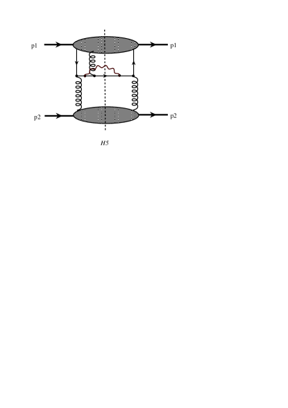
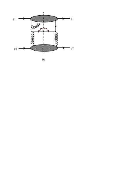
Figure 2: The typical Feynman diagrams to check the QCD gauge invariance.

5 Conclusions

We explore the QCD gauge invariance of the hadron tensor for the direct photon production in two hadron collision where one of hadrons is transversely polarized. We argue the effects which lead to the soft breaking of factorization by inspection of the QCD gauge invariance. We demonstrate that the initial or final state interactions in diagrams define the different prescriptions in the gluonic poles. Moreover, the different prescriptions are needed to ensure the QCD gauge invariance. This situation can be treated as a soft breaking of the universality condition resulting in factorization breaking.

Acknowledgements

We would like to thank I.O. Cherednikov, A.V. Efremov, D. Ivanov and L. Szymanowski for useful discussions and correspondence. This work is partly supported by the HL program.

References

- [1] I. V. Anikin and O. V. Teryaev, Phys. Lett. B 690, 519 (2010) [arXiv:1003.1482 [hep-ph]]; I. V. Anikin and O. V. Teryaev, J. Phys. Conf. Ser. 295, 012057 (2011) [arXiv:1011.6203 [hep-ph]].
- [2] D. Boer and J. w. Qiu, Phys. Rev. D 65, 034008 (2002) [arXiv:hep-ph/0108179].
- [3] G. Re Calegari and P. G. Ratcliffe, Eur. Phys. J. C 74, 2769 (2014) [arXiv:1307.5178 [hep-ph]].
- [4] B. Pire and J. P. Ralston, Phys. Rev. D 28, 260 (1983).
- [5] R. D. Carlitz and R. S. Willey, Phys. Rev. D 45, 2323 (1992).
- [6] A. Brandenburg, D. Mueller and O. V. Teryaev, Phys. Rev. D 53, 6180 (1996) [arXiv:hep-ph/9511356].
- [7] A. P. Bakulev, N. G. Stefanis and O. V. Teryaev, Phys. Rev. D 76, 074032 (2007) [arXiv:0706.4222 [hep-ph]].
- [8] A. V. Radyushkin, Phys. Rev. D 80, 094009 (2009) [arXiv:0906.0323 [hep-ph]].
- [9] M. V. Polyakov, JETP Lett. 90, 228 (2009) [arXiv:0906.0538 [hep-ph]].
- [10] S. V. Mikhailov and N. G. Stefanis, Mod. Phys. Lett. A 24, 2858 (2009) [arXiv:0910.3498 [hep-ph]].
- [11] A. Brandenburg, S. J. Brodsky, V. V. Khoze and D. Mueller, Phys. Rev. Lett. 73, 939 (1994) [arXiv:hep-ph/9403361].
- [12] N. Hammon, O. Teryaev and A. Schafer, Phys. Lett. B 390, 409 (1997) [arXiv:hep-ph/9611359].
- [13] D. Boer, P. J. Mulders and O. V. Teryaev, arXiv:hep-ph/9710525; Phys. Rev. D 57, 3057 (1998) [arXiv:hep-ph/9710223].
- [14] O. V. Teryaev, RIKEN Rev. 28, 101 (2000).
- [15] P. G. Ratcliffe and O. Teryaev, Mod. Phys. Lett. A 24, 2984 (2009) [arXiv:0910.5348 [hep-ph]].
- [16] H. G. Cao, J. P. Ma and H. Z. Sang, Commun. Theor. Phys. 53, 313 (2010) [arXiv:0901.2966 [hep-ph]].
- [17] J. Zhou, F. Yuan and Z. T. Liang, Phys. Rev. D 81, 054008 (2010) [arXiv:0909.2238 [hep-ph]].
- [18] J. P. Ma and Q. Wang, Eur. Phys. J. C 37, 293 (2004) [arXiv:hep-ph/0310245].
- [19] I. V. Anikin and O. V. Teryaev, “New contributions to gluon poles in direct photon production,” arXiv:1501.04536 [hep-ph].
- [20] V. Barone, A. Drago and P. G. Ratcliffe, Phys. Rept. 359, 1 (2002) [arXiv:hep-ph/0104283].
- [21] I. V. Anikin and O. V. Teryaev, Phys. Part. Nucl. Lett. 6, 3 (2009) [arXiv:hep-ph/0608230];
- [22] A. V. Efremov and A. V. Radyushkin, Theor. Math. Phys. 44, 774 (1981) [Teor. Mat. Fiz. 44, 327 (1980)].
- [23] S. V. Ivanov, G. P. Korchemsky and A. V. Radyushkin, Yad. Fiz. 44, 230 (1986) [Sov. J. Nucl. Phys. 44, 145 (1986)]; S. V. Ivanov and G. P. Korchemsky, Phys. Lett. B 154, 197 (1985); S. V. Ivanov, Fiz. Elem. Chast. Atom. Yadra 21, 75 (1990).
- [24] I. V. Anikin, D. Y. Ivanov, B. Pire, L. Szymanowski and S. Wallon, Nucl. Phys. B 828, 1 (2010) [arXiv:0909.4090 [hep-ph]].
- [25] A. V. Radyushkin, Phys. Rev. D 56, 5524 (1997) [arXiv:hep-ph/9704207].
- [26] V. M. Braun, D. Y. Ivanov, A. Schafer and L. Szymanowski, Nucl. Phys. B 638, 111 (2002) [arXiv:hep-ph/0204191].
- [27] N. N. Bogolyubov and D. V. Shirkov, “Introduction To The Theory Of Quantized Fields,” Intersci. Monogr. Phys. Astron. 3, 1 (1959).
- [28] Y. Koike and K. Tanaka, arXiv:0907.2797 [hep-ph].