On the equivalence between continuum and car-following models of traffic flow

Abstract

Recently different formulations of the first-order Lighthill-Whitham-Richards (LWR) model have been identified in different coordinates and state variables. However, there exists no systematic method to convert higher-order continuum models into car-following models and vice versa. In this study we propose a simple method to enable systematic conversions between higher-order continuum and car-following models in two steps: equivalent transformations of variables between Eulerian and Lagrangian coordinates, and finite difference approximations of first-order derivatives in Lagrangian coordinates. With the method, we derive higher-order continuum models from a number of well-known car-following models. We also derive car-following models from higher-order continuum models. For general second-order models, we demonstrate that the car-following and continuum formulations share the same fundamental diagram, but the string stability condition of a car-following model is different from the linear stability condition of a continuum model. This study reveals relationships between many existing models and also leads to a number of new models.

Keywords: Eulerian coordinates; Lagrangian coordinates; Primary models; Secondary models; First-order models; Higher-order models; Continuum models; Car-following models; Fundamental diagram; Stability.

1 Introduction

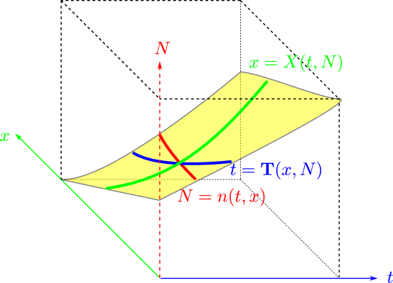
Figure 1: The $x-t-N$ surface for a traffic stream

In the three-dimensional representation of traffic flow (Makigami et al.,, 1971), as shown in Figure 1, the evolution of a traffic stream can be captured by a surface in a three-dimensional space of time $t$, location $x$, whose positive direction is the same as the traffic direction, and vehicle number $N$, which is the cumulative number of vehicles passing location $x$ at $t$ after a reference vehicle (Moskowitz,, 1965). We call these primary variables of traffic flow. In the figure, the red curve,

$$N=n(t,x),$$ (1a)

represents the $$x-t N$$ trajectory of vehicle , which can be collected with GPS devices; the green curve,

$$x=X(t,N),$$ (1b)

represents the cumulative number of vehicles $$N t x$$ before at location , which can be extracted from vehicle counts of a loop detector; and the blue curve,

$$t={{\bf T}}(x,N),$$ (1c)

represents the number of vehicles $N$ downstream to $x$ at time $t$, which can be counted from a camera snapshot. Among the three primary variables, the two independent variables form a coordinate system and the dependent one is the state variable. In particular, $(t,x)$ form the Eulerian coordinates, and $(t,N)$ the Lagrangian coordinates.

The goal of a traffic flow model is to determine the surface from given initial, boundary, or internal conditions. It is usually written as a partial differential equation or a corresponding difference form. We call a traffic flow model primary if one of the three primary variables is the unknown state variable, and the order of the model is the maximum order of partial derivatives. In contrast, if a partial derivative of a primary variable is used as the unknown state variable, we call the model secondary. In this study, we will categorize traffic flow models according to their coordinates, state variables, and orders.

In the Eulerian coordinates, we can define traffic density $k=-n_{x}$ and flow-rate $q=n_{t}$, where the subscripts mean partial derivatives. Then the celebrated LWR model (Lighthill and Whitham,, 1955; Richards,, 1956) is a partial differential equation in $k$:

$${\frac{\partial{k}}{\partial{t}}}+{\frac{\partial{\phi(k)}}{\partial{x}}} = 0,$$ (2)

which is a hyperbolic conservation law (Lax,, 1972). Thus, the LWR model is a first-order secondary model in the Eulerian coordinates, abbreviated as the E-S-1 model. The model can be derived from the following three rules:

• Fundamental law of traffic flow: speed $v=\frac{q}{k}$;

• Conservation of traffic flow: $k_{t}+q_{x}=0$;

• Fundamental diagram of flow-density relation:

  $$q = \phi(k).$$ (3)

In particular, the following triangular fundamental diagram has been shown to match observations in steady traffic well (Munjal et al.,, 1971; Haberman,, 1977; Newell,, 1993):

$$\phi(k) = \min\{v_{f}k,w(k_{j}-k)\},$$

where $v_{f}$ is the free-flow speed, $-w$ the shock wave speed in congested traffic, and $k_{j}$ the jam density. The Greenshields fundamental diagram is (Greenshields,, 1935)

$$\phi(k) = v_{f}k(1-k/k_{j}).$$

In (Newell,, 1993), the E-P-1 model, i.e., the first-order primary traffic flow model in the Eulerian coordinates, was first discussed:

$$n_{t}-\phi(-n_{x}) = 0,$$ (4)

which is a Hamilton-Jacobi equation (Evans,, 1998). This model can be numerically solved with the variational principle (Daganzo, 2005a, ; Daganzo, 2005b, ), or the Hopf-Lax formula (Claudel and Bayen,, 2010). In (Daganzo, 2006b, ), the L-P-1 formulation of the LWR model, i.e., the first-order primary formulation in the Lagrangian coordinates, was derived based on the inverse function theorem as

$$X_{t}-\theta(-X_{N}) = 0,$$ (5)

which is also a Hamilton-Jacobi equation. If we denote the spacing by $S=-X_{N}$, then the speed-spacing relation is

$$\theta(S)=S\phi(1/S).$$ (6)

In particular, for the triangular fundamental diagram

$$\theta(S)=\min\{v_{f},w(k_{j}S-1)\};$$

and for the Greenshields fundamental diagram

$$\theta(S)=v_{f}(1-\frac{1}{Sk_{j}}).$$

Further in (Daganzo, 2006b, ; Daganzo, 2006a, ), various discrete forms of (5) was obtained based on the variational principle. In particular, Newell’s car-following model is shown to be a discrete form of (5) with the triangular fundamental diagram. In (Leclercq et al.,, 2007), the L-S-1 formulation was derived as a hyperbolic conservation law and numerically solved with the Godunov method (Godunov,, 1959). More recently, in (Laval and Leclercq,, 2013), the equivalent primary and secondary formulations in the $(x,N)$-coordinates, called $T$-models, were derived and solved. In summary, all the primary formulations of the LWR model are Hamilton-Jacobi equations and can be solved with the variational principle, the Hopf-Lax formula, or other techniques (Evans,, 1998); and all the secondary formulations are hyperbolic conservation laws and can be solved with the Godunov scheme.

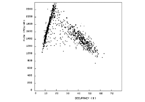
Figure 2: An observed flow-occupancy relation (Hall et al.,, 1986)

An equilibrium flow-density relationship (3) has been derived from various car-following models in steady states (Gazis et al.,, 1961; Haberman,, 1977, Chapter 61) and verified with empirical observations (Del Castillo and Benitez,, 1995; Cassidy,, 1998). However, in reality, traffic can be in non-equilibrium states, and the flow-density or flow-occupancy relations are not unique, as shown in Figure 2. In such non-equilibrium traffic, instability and hysteresis phenomena have been observed (Newell,, 1965; Treiterer and Myers,, 1974; Sugiyama et al.,, 2008). In order to capture such non-equilibrium features of traffic flow, researchers have introduced numerous higher-order continuum models: in (e.g. Payne,, 1971; Whitham,, 1974; Zhang,, 1998; Aw and Rascle,, 2000; Zhang,, 2002), the conservation equation is coupled with one or more equations in speed or other variables. There have been extensive discussions on theoretical consistency of some higher-order models (Daganzo,, 1995; Lebacque et al.,, 2007; Helbing and Johansson,, 2009; Zhang,, 2009; Helbing,, 2009) and on the stability and other properties (Kerner and Konhäuser,, 1994; Li,, 2001; Jin and Zhang,, 2003). Note that, however, these models are still limited, as they are just capable of explaining a subset of many non-equilibrium phenomena (Kerner,, 2004). Non-equilibrium traffic phenomena have also been successfully modeled with microscopic car-following models since 1950’s in the transportation field (Pipes,, 1953; Herman et al.,, 1959) and in the physics field, as traffic systems can be considered many-particle systems (Bando et al.,, 1995). Recently stability and other properties of car-following models have been subjects of some mathematical studies (Wilson,, 2001; Orosz and Stépán,, 2006). Reviews of various car-following models are available in (Rothery,, 1992; Brackstone and McDonald,, 1999; Chowdhury et al.,, 2000; Helbing,, 2001). In the literature, many higher-order continuum models have been derived from car-following models using the method of Taylor series expansion (e.g. Payne,, 1971; Del Castillo et al.,, 1994; Zhang,, 1998; Berg et al.,, 2000; Zhang,, 2002; Jiang et al.,, 2002). However, the derivation process is model specific, and different approximation methods can lead to different continuum models for the same car-following model. In addition, such a method cannot be used to derive car-following models from continuum models.

From the studies on different formulations of the LWR model in (Daganzo, 2006a, ; Daganzo, 2006b, ; Leclercq et al.,, 2007; Laval and Leclercq,, 2013), we can see that car-following models can be considered as discrete primary formulations in the Lagrangian coordinates, and continuum models as secondary formulations in the Eulerian coordinates. Based on this observation, in this study we will develop a systematic method for conversions between higher-order continuum models and car-following models. However, the framework is different from that for the first-order models: first, the higher-order L-P models are no longer Hamilton-Jacobi equations, and the variational principle or the Hopf-Lax formula cannot be applied to obtain car-following models from the L-P models; second, as higher-order derivatives of the primary variables are involved, the inverse function theorem cannot be used to transform variables between Eulerian and Lagrangian coordinates. To resolve the first difficulty, we use simple finite difference methods to derive car-following models from L-P models, since a driver’s car-following behavior is only impacted by its leader; to resolve the second difficulty, we systematically derive the transformations of related variables between Eulerian and Lagrangian coordinates. The conversion method consists of two components: finite difference approximations of L-P derivatives, and transformations between E-S and L-P variables. With this method, we will derive continuum formulations of car-following models and vice versa. We will be able to reveal relationships between some high-order models and also derive new continuum and car-following models from existing ones. We will also examine the equivalence between general second-order continuum and car-following models in their steady-state speed-density relations and stability of steady states.

The rest of the paper is organized as follows. In Section 2, we present a method for conversions between continuum and car-following models and apply it to the first-order models. In Section 3, we derive continuum formulations of some car-following models. In Section 4, we derive car-following formulations of higher-order continuum models. In Section 5, we examine the equivalence between continuum and car-following models. In Section 6, we discuss some future directions.

2 A systematic conversion method

In this section we present a systematic method for conversions between car-following and continuum models. First, we present transformations between E-S and L-P variables, which lead to equivalent E-S and L-P formulations of a traffic flow model. Second, we present finite difference approximations of L-P. derivatives

2.1 Transformations between E-S and L-P variables

In E-S models, variables include $k$, $q$, $v$, and their derivatives with respect to $x$ and $t$; in L-P models, variables include $X$ and its derivatives with respect to $N$ and $t$. In this subsection, we establish the equivalence between E-S and L-P models through transformations between Eulerian and Lagrangian variables.

For a physical variable, we denote it by $F(t,N)$ in the Lagrangian coordinates and by $f(t,x)$ in the Eulerian coordinates. Then from (1a) we have

$$f(t,x) = F(t,N)=F(t,n(t,x)),$$ (7)

which leads to

$$f_{t} = F_{t}+F_{N}n_{t},$$ (8a)

$$f_{x} = F_{N}n_{x}.$$ (8b)

In particular, if we let $f(t,x)=x$ and $F(t,N)=X(t,N)$, then from (8) we have

$$0 = X_{t}+X_{N}n_{t},$$

$$1 = X_{N}n_{x},$$

which lead to

$$q = n_{t}=-\frac{X_{t}}{X_{N}},$$ (9a)

$$-k = n_{x}=\frac{1}{X_{N}}.$$ (9b)

Substituting (9) into (8), we obtain the transformation of derivatives in the Eulerian coordinates into those in the Lagrangian coordinates:

$$f_{t} = F_{t}-F_{N}\frac{X_{t}}{X_{N}},$$ (10a)

$$f_{x} = F_{N}\frac{1}{X_{N}}.$$ (10b)

We can repeatedly use (10) to transform higher-order derivatives from E-coordinate to L-coordinate. For example, if we denote $$g=f_{t} G=F_{t}-F_{N}\frac{X_{t}}{X_{N}}$$ and , then we have

$$f_{tt} = g_{t}=G_{t}-G_{N}\frac{X_{t}}{X_{N}}=F_{tt}-2F_{Nt}\frac{X_{t}}{X_{N}}+F_{NN}(\frac{X_{t}}{X_{N}})^{2}-F_{N}\frac{X_{tt}X_{N}^{2}-X_{t}^{2}X_{NN}}{X_{N}^{3}}.$$ (10c)

Similarly, we have

$$f_{tx} = (F_{tN}-F_{NN}\frac{X_{t}}{X_{N}}-F_{N}\frac{X_{tN}X_{N}-X_{t}X_{NN}}{X_{N}^{2}})\frac{1}{X_{N}},$$ (10d)

$$f_{xx} = \frac{F_{NN}X_{N}-F_{N}X_{NN}}{X_{N}^{3}}.$$ (10e)

In particular, when $f(t,x)=n(t,x)$ and $F(t,N)=N$, we have $q_{t}=n_{tt}=-\frac{X_{tt}X_{N}^{2}-X_{t}^{2}X_{NN}}{X_{N}^{3}}$, $q_{x}=-k_{t}=n_{tx}=-\frac{X_{tN}X_{N}-X_{t}X_{NN}}{X_{N}^{3}}$, and $-k_{x}=n_{xx}=-\frac{X_{NN}}{X_{N}^{3}}$.

Similarly we can transform a variable and its derivatives from the Lagrangian coordinates to the Eulerian coordinates as follows:

$$F(t,N) = f(t,X(t,N)),$$ (11a)

$$F_{t} = f_{t}-f_{x}\frac{n_{t}}{n_{x}}=f_{t}+vf_{x},$$ (11b)

$$F_{N} = f_{x}\frac{1}{n_{x}}=-f_{x}\frac{1}{k},$$ (11c)

and

$$F_{tt} = f_{tt}+2vf_{tx}+v^{2}f_{xx}+(v_{t}+vv_{x})f_{x},$$ (11d)

$$F_{tN} = -(f_{tx}+vf_{xx}+v_{x}f_{x})\frac{1}{k},$$ (11e)

$$F_{NN} = (kf_{xx}-k_{x}f_{x})\frac{1}{k^{3}}.$$ (11f)

In particular, when $F(t,N)=X$ and $f(t,x)=x$, we have $X_{t}=v$, $X_{N}=-\frac{1}{k}$, $X_{tt}=v_{t}+vv_{x}$, $X_{tN}=-\frac{v_{x}}{k}$, and $X_{NN}=-\frac{k_{x}}{k^{3}}$.

In Table 1, where $A=V_{t}$ and $a=v_{t}+vv_{x}$, we summarize transformations between L-P and E-S variables. In the table, variables are divided into three groups: the first group are for $k,q,v$; the second group for simple derivatives of $k$ and $v$ in the Eulerian coordinates; and the third group for simple derivatives of $X$ in the Lagrangian coordinates. The equivalent variables in E-P and L-S models can be easily obtained through changes of variables but are omitted here.

Variables	L-P	E-S
Density	$-\frac{1}{X_{N}}$	$k$
Speed	$X_{t}$	$v$
Flow-rate	$-\frac{X_{t}}{X_{N}}$	$q$
Speed rate	$X_{tt}-\frac{X_{t}}{X_{N}}X_{tN}$	$v_{t}$
Speed gradient	$\frac{1}{X_{N}}X_{tN}$	$v_{x}$
Speed curvature	$\frac{X_{tNN}X_{N}-X_{tN}X_{NN}}{X_{N}^{3}}$	$v_{xx}$
Density rate	$\frac{X_{tN}X_{N}-X_{t}X_{NN}}{X_{N}^{3}}$	$k_{t}$
Density gradient	$\frac{X_{NN}}{X_{N}^{3}}$	$k_{x}$
Acceleration rate	$X_{tt}$	$v_{t}+vv_{x}$
Jerk	$X_{ttt}$	$a_{t}+va_{x}$
Speed difference	$X_{tN}$	$-\frac{v_{x}}{k}$
Spacing difference	$X_{NN}$	$-\frac{k_{x}}{k^{3}}$

Table 1: Transformations between E-S and L-P variables

2.2 Finite difference approximations of L-P derivatives

In traffic flow, information travels in the increasing direction of $N$; that is, the following vehicles have to adjust their behaviors according to the leading vehicles. Therefore, a simple upwind scheme can be used to numerically solve the L-P formulation as follows: first, we approximate the derivatives with respect to vehicle number by finite differences

$$F_{N}(t,N) \approx \frac{F(t,N)-F(t,N-\Delta N)}{\Delta N},$$

In particular, when $\Delta N=1$, a vehicle just follows its immediate leader, and we have

$$F_{N}(t,N) \approx F(t,N)-F(t,N-1).$$ (12)

Similarly we can obtain the vehicle-discrete forms of speed and spacing differences

$$X_{N}(t,N) \approx X(t,N)-X(t,N-1),$$

$$X_{tN}(t,N) \approx X_{t}(t,N)-X_{t}(t,N-1),$$

$$X_{NN}(t,N) \approx X(t,N)+X(t,N-2)-2X(t,N-1).$$

Note that the right-hand sides of the approximations are discrete in vehicle number but still continuous in time. Such vehicle-difference L-P variables are used in time-continuous car-following models.

Furthermore we can use the forward difference to replace the derivatives with respect to time in the vehicle-difference forms:

$$F_{t}(t,N) \approx \frac{F(t+{\Delta t},N)-F(t,N)}{{\Delta t}},$$ (13)

where ${\Delta t}$ should satisfy the CFL condition (Courant et al.,, 1928; Leclercq et al.,, 2007): ${\Delta t}\leq\max|\theta^{\prime}(S)|$ with $\Delta N=1$, which can be derived from the L-S formulations. In particular, for the triangular fundamental diagram, we have ${\Delta t}\leq\frac{1}{wk_{j}}$. Intuitively, information cannot pass for more than one vehicle during a time interval; i.e., a leading vehicle cannot impact the behavior of more than one vehicle, its follower, during a time interval. With both (12) and (13) we can obtain time-discrete car-following models from the L-P formulations.

2.3 A two-way method

Based on the transformations between E-S and L-P variables, we can then obtain equivalent E-S and L-P formulations when one of them is given. From the finite difference approximations of L-P derivatives, we can convert L-P formulations into car-following models and vice versa. Therefore, conversions between continuum and car-following models can be done in two steps, whose order depends on the direction of conversion. Note that the resulting E-S and L-P models are equivalent, but the car-following models are just approximately equivalent to the L-P models, subject to errors between derivatives and finite differences.

Here we apply the method to derive equivalent time-continuous and time-discrete car-following models of the LWR model, the first-order continuum model, by discretizing (5):

$$X_{t}(t,N) = \theta(X(t,N-1)-X(t,N)),$$ (14)

$$X(t+{\Delta t},N) = X(t,N)+{\Delta t}\theta(X(t,N-1)-X(t,N)).$$ (15)

In particular, for the triangular fundamental diagram, we have

$$X_{t}(t,N) = \min\{v_{f},\frac{1}{\tau}(X(t,N-1)-X(t,N)-S_{j})\},$$ (16)

$$X(t+{\Delta t},N) = X(t,N)+{\Delta t}\min\{v_{f},\frac{1}{\tau}(X(t,N-1)-X(t,N)-S_{j})\},$$ (17)

where $\tau=\frac{1}{wk_{j}}$ is the time gap, and $S_{j}=1/k_{j}$ the jam spacing. Here the congested part of the time-continuous car-following model, (16), is essentially the same as the original Pipes car-following model, Equation 2.3 in (Pipes,, 1953). If the minimum time ${\Delta t}=\tau$ in the time-discrete Pipes model, (17), then we have

$$X(t+\tau,N) = \min\{X(t,N)+\tau v_{f},X(t,N-1)-S_{j}\},$$ (18)

which is Newell’s car-following model (Newell,, 2002; Daganzo, 2006a, ). From the Hopf-Lax formula, we can show that the model is accurate subject to the assumption of uniform spacings between two consecutive vehicles (Evans,, 1998).

3 Continuum formulations of higher-order car-following models

In this section, we apply the method in the preceding section to derive continuum formulations of higher-order time-continuous car-following models. In the first step, we approximate finite differences by partial derivatives with respect to vehicle numbers; in the second step, we convert L-P models to E-S continuum models.

3.1 Second-order models

In the literature, a large number of time-continuous car-following models have been developed to calculate a follower’s acceleration rate from its speed, spacing, and speed difference and can be written in the following form:

$$X_{tt}(t,N) = \Psi(X_{t}(t,N),\Delta X(t,N),\Delta X_{t}(t,N)),$$ (19)

where vehicle $N$ follows vehicle $N-1$, the spacing $\Delta X(t,N)=X(t,N-1)-X(t,N)$, and the speed difference $\Delta X_{t}(t,N)=X_{t}(t,N-1)-X_{t}(t,N)$.

In the first step, from (12), we can replace the discrete spacing $\Delta X(t,N)$ by the continuous spacing $-X_{N}$, and the discrete speed difference $\Delta X_{t}(t,N)$ by the continuous speed difference $-X_{tN}$. Then we obtain the corresponding L-P formulation of the car-following model, (19):

$$X_{tt} = \Psi(X_{t},-X_{N},-X_{tN}),$$ (20)

which is a second-order model as the highest order of derivatives is two. In the second step, from Table 1 we obtain the following E-S formulation:

$$v_{t}+vv_{x} = \Psi(v,\frac{1}{k},\frac{v_{x}}{k}),$$ (21a)

which, coupled with the conservation equation,

$$k_{t}+(kv)_{x}=0,$$ (21b)

forms a second-order continuum model (Payne,, 1971; Whitham,, 1974).

The following are some examples:

1. The linear General Motors model without delay, which was derived based on the stimulus-response principle (Pipes,, 1953; Gazis et al.,, 1959), can be written as

   $$X_{tt}(t,N) = \frac{1}{T}\Delta X_{t}(t,N),$$ (22)

   where $T>0$ is the reaction time. Thus $\Psi(v,\frac{1}{k},\frac{v_{x}}{k})=\frac{1}{T}\frac{v_{x}}{k}$, and the second-order continuum model is (we omit the conservation equation (21b) hereafter.)

   $$v_{t}+\left(v-\frac{1}{T}\frac{1}{k}\right)v_{x} = 0.$$ (23)

2. The nonlinear General Motors model without delay (Gazis et al.,, 1961) can be written as:

   $$X_{tt}(t,N) = a\frac{X_{t}^{m}\Delta X_{t}(t,N)}{[\Delta X(t,N)]^{l}},$$

   where $m$ and $l$ are natural numbers, and $a>0$. Thus $\Psi(v,\frac{1}{k},\frac{v_{x}}{k})=av^{m}k^{l-1}v_{x}$, and the second-order continuum model is

   $$v_{t}+\left(v-av^{m}k^{l-1}\right)v_{x} = 0.$$ (24)

3. The Optimal Velocity Model (OVM) without delay (Bando et al.,, 1995) can be written as:

   $$X_{tt}(t,N) = \frac{1}{T}(\theta(\Delta X(t,N))-X_{t}(t,N)).$$ (25)

   Thus $\Psi(v,\frac{1}{k},\frac{v_{x}}{k})=\frac{1}{T}(\theta(\frac{1}{k})-v)$, and the second-order continuum model is

   $$v_{t}+vv_{x} = \frac{1}{T}\left(\theta(\frac{1}{k})-v\right).$$ (26)

   Note that the model in (Newell,, 1961), $X_{t}(t+T,N)=\theta(\Delta X(t,N))$, is equivalent to the Optimal Velocity Model if we approximate $X_{t}(t+T,N)$ by its Taylor series expansion: $X_{t}(t,N)+TX_{tt}(t,N)$.

4. The Generalized Force Model (GFM) (Helbing and Tilch,, 1998) can be written as:

   $$X_{tt}(t,N) = \frac{1}{T}(\theta(\Delta X(t,N))-X_{t}(t,N))-\frac{\Delta X_{t}(t,N)\Theta(\Delta X_{t}(t,N))}{T^{\prime}}e^{-[\Delta X(t,N)-(d+\tau X_{t}(t,N))]/R^{\prime}},$$

   where $T$ is the acceleration time, $T^{\prime}<T$ the braking time, $d$ the minimal vehicle distance, $\tau$ the safe time headway (time gap), $R^{\prime}$ the range of the braking interaction, and $\Theta(\cdot)$ the Heaviside function. Thus $\Psi(v,\frac{1}{k},\frac{v_{x}}{k})=\frac{1}{T}(\theta(\frac{1}{k})-v)-\frac{v_{x}\Theta(v_{x}/k)}{T^{\prime}k}e^{-[1/k-(d+\tau v)]/R^{\prime}}$, and the second-order continuum model is

   $$v_{t}+\left(v+\frac{1}{T^{\prime}}\frac{\Theta(v_{x}/k)}{k}e^{-[1/k-(d+\tau v)]/R^{\prime}}\right)v_{x} = \frac{1}{T}\left(\theta(\frac{1}{k})-v\right).$$ (27)

5. The Intelligent Driver Model (IDM) (Treiber et al.,, 2000) can be written as:

   $$X_{tt}(t,N) = a\left[1-\left(\frac{X_{t}(t,N)}{v_{f}}\right)^{\delta}-\left(\frac{d+\tau X_{t}(t,N)+\frac{X_{t}(t,N)\Delta X_{t}(t,N)}{2\sqrt{ab}}}{\Delta X(t,N)}\right)^{2}\right],$$

   where $a$ is the maximum acceleration rate, $\delta$ the acceleration exponent, $b$ the desired deceleration rate, $\tau$ the safe time headway (time gap), and $d$ the minimal vehicle distance. Thus $\Psi(v,\frac{1}{k},\frac{v_{x}}{k})=a\left[1-(\frac{v}{v_{f}})^{\delta}-(\frac{k}{k_{j}}+\tau kv+\frac{vv_{x}}{2\sqrt{ab}})^{2}\right]$, and the second-order continuum model is

   $$v_{t}+vv_{x} = a\left[1-\left(\frac{v}{v_{f}}\right)^{\delta}-\left(dk+\tau kv+\frac{vv_{x}}{2\sqrt{ab}}\right)^{2}\right].$$ (28)

6. The Full Velocity Difference Model (FVDM) (Jiang et al.,, 2001) is a combination of the linear General Motors model and the Optimal Velocity Model and can be written as:

   $$X_{tt}(t,N) = \frac{1}{T}(\theta(\Delta X(t,N))-X_{t}(t,N))+\lambda\Delta X_{t}(t,N),$$ (29)

   where $T$ is the reaction time, and $\lambda$ the sensitivity coefficient. Thus $\Psi(v,\frac{1}{k},\frac{v_{x}}{k})=\frac{1}{T}(\theta(\frac{1}{k})-v)+\lambda\frac{v_{x}}{k}$, and the second-order continuum model is

   $$v_{t}+\left(v-\frac{\lambda}{k}\right)v_{x} = \frac{1}{T}\left(\theta(\frac{1}{k})-v\right).$$ (30)

Among the six continuum models, (23)-(30), the one for the linear General Motors model, (23), is a special case of the Aw-Rascle-Zhang model (Aw and Rascle,, 2000; Zhang,, 2002); the one for the Optimal Velocity model, (26), appeared in (Phillips,, 1979); the one for the Full Velocity Difference Model, (30), is a special case of the Aw-Rascle-Greenberg model (Aw and Rascle,, 2000; Greenberg,, 2001); but, to the best of our knowledge, the other three models are new.

3.2 Third-order models

In some second-order car-following models, there is a delay term in the acceleration rate:

$$X_{tt}(t+T^{\prime},N) = \Psi(X_{t}(t,N),\Delta X(t,N),\Delta X_{t}(t,N)).$$ (31)

If approximating $X_{tt}(t+T^{\prime},N)$ by its Taylor series expansion, $X_{tt}(t,N)+T^{\prime}X_{ttt}(t,N)$, we then obtain a third-order car-following model:

$$X_{ttt}(t,N) = \frac{1}{T^{\prime}}[\Psi(X_{t}(t,N),\Delta X(t,N),\Delta X_{t}(t,N))-X_{tt}(t,N)].$$ (32)

By using the same method in the preceding subsection, we can then derive the following third-order continuum model:

$$k_{t}+(kv)_{x} = 0,$$ (33a)

$$v_{t}+vv_{x} = a,$$ (33b)

$$a_{t}+va_{x} = \frac{1}{T^{\prime}}\left[\Psi(v,\frac{1}{k},\frac{v_{x}}{k})-a\right],$$ (33c)

where $$a a_{t}+va_{x}$$ is the acceleration rate, and the jerk.

For examples, we can derive such continuum models for the General Motors model with delay (Gazis et al.,, 1959, 1961) and the Optimal Velocity Model with delay (Bando et al.,, 1998). Further higher-order models can also be derived by using this method.

4 Car-following formulations of higher-order continuum models

In this section, we apply the conversion method in Section 2 to derive car-following models from higher-order continuum models.

4.1 A review of higher-order continuum models

We give a brief review of existing second-order continuum models and categorized them into four families. All second-order models consist of the conservation equation, (21b), and an additional equation in speed. Here we just list the equation in speed and denote the speed-density relation by $\eta(k)=\theta(1/k)$:

1. The Phillips family:

   • (Phillips,, 1979): $v_{t}+vv_{x}=\frac{1}{T}(\eta(k)-v)$;

   • (Ross,, 1988): $v_{t}+vv_{x}=\frac{1}{T}(v_{f}-v)$, which was shown to be unrealistic in (Newell,, 1989);

   • (Liu et al.,, 1998): $v_{t}=\frac{1}{T(k)}(\eta(k)-v)$, in which the relaxation time $T(k)$ is a function of density $k$.

2. The Payne family:

   • (Payne,, 1971): $v_{t}+vv_{x}-\frac{\eta^{\prime}(k)}{2Tk}k_{x}=\frac{1}{T}(\eta(k)-v)$;

   • (Whitham,, 1974): $v_{t}+vv_{x}+\frac{c_{0}^{2}}{k}k_{x}=\frac{1}{T}(\eta(k)-v)$;

   • (Phillips,, 1979): $v_{t}+vv_{x}+\frac{p^{\prime}(k)}{k}k_{x}=\frac{1}{T}(\eta(k)-v)$, where $p(k)$ is the traffic pressure function;

   • (Kuhne,, 1987; Kuhne and Michalopoulos,, 1992; Kerner and Konhäuser,, 1993): $v_{t}+vv_{x}+\frac{c_{0}^{2}}{k}k_{x}=\frac{1}{T}(\eta(k)-v)+\frac{\mu_{0}}{k}v_{xx}$, which has a viscous term;

   • (Zhang,, 1998): $v_{t}+vv_{x}+\frac{(k\eta^{\prime}(k))^{2}}{k}k_{x}=\frac{1}{T}(\eta(k)-v)$.

3. The Aw-Rascle family:

   • (Aw and Rascle,, 2000):

     $$v_{t}+(v-kp^{\prime}(k))v_{x}=0;$$ (34)

   • (Zhang,, 2002):

     $$v_{t}+(v+k\eta^{\prime}(k))v_{x}=0;$$ (35)

   • (Greenberg,, 2001): $v_{t}+(v+k\eta^{\prime}(k))v_{x}=\frac{1}{T}(\eta(k)-v)$;

   • (Jiang et al.,, 2002):

     $$v_{t}+(v-c_{0})v_{x}=\frac{1}{T}(\eta(k)-v);$$ (36)

   • (Xue and Dai,, 2003): $v_{t}+(v+k\frac{t_{r}}{T(k)}\eta^{\prime}(k))v_{x}=\frac{1}{T(k)}(\eta(k)-v)$, where $t_{r}$ is driver’s reaction time.

4. The Zhang family:

   • (Zhang,, 2003): $v_{t}+(v+2\beta c(k))v_{x}+\frac{c^{2}(k)}{k}k_{x}=\frac{1}{T}(\eta(k)-v)+\mu(k)v_{xx}$, where $c(k)=k\eta^{\prime}(k)$, $\mu(k)=2\beta Tc^{2}(k)$.

From these models we have the following observations:

• Models of the Phillips family are the simplest: those of the Payne-Whitham family have one extra term with the density gradient $k_{x}$; those of the Aw-Rascle family have one extra term with the speed gradient $v_{x}$; and those of the Zhang family have both.

• Most models have the total derivative in $v$, $v_{t}+vv_{x}$, and some just have the partial derivative, $v_{t}$.

• Some models have the relaxation term, $\frac{1}{T}(\eta(k)-v)$, and some do not.

• Some models have the viscous term $v_{xx}$, but most do not.

In the literature, third- or even higher-order continuum models have been proposed (Phillips,, 1979; Helbing,, 1995, 1996; Colombo, 2002a, ; Colombo, 2002b, ). But in this study we focus on the second-order models.

4.2 Car-following models of second-order continuum models

Given a continuum model, in the first step, we convert them into L-P formulations by following Table 1; in the second step, we approximate partial derivatives with respect to vehicle numbers by finite differences. In this subsection we only use the car-following models of the Aw-Rascle family as examples.

Even though the continuum formulations of General Motors and Full Velocity Difference models belong to the Aw-Rascle family, we can obtain more general car-following models of the following general Aw-Rascle model:

$$v_{t}+(v-kp^{\prime}(k))v_{x}=\frac{1}{T(k)}(\eta(k)-v).$$ (37)

First, from Table 1 we can have the L-P formulation of (37):

$$X_{tt} = \frac{1}{T(-1/X_{N})}(\theta(-X_{N})-X_{t})-p^{\prime}(-1/X_{N})\frac{X_{tN}}{X_{N}^{2}}.$$ (38)

Further replacing $-X_{N}$ by $\Delta X(t,N)$ and $-X_{tN}$ by $\Delta X_{t}(t,N)$, we obtain the following car-following model:

$$X_{tt}(t,N) = \frac{1}{T(1/\Delta X(t,N))}(\theta(\Delta X(t,N))-X_{t}(t,N))+p^{\prime}(1/\Delta X(t,N))\frac{\Delta X_{t}(t,N)}{\Delta X(t,N)^{2}}.$$ (39)

The new car-following model (39) combines a generalized Optimal Velocity model (the first term on the right-hand side) and a nonlinear General Motors model (the second term on the right-hand side). This model is also in the form of (19).

For example, the car-following formulation of the Aw-Rascle-Zhang model, (35), is

$$X_{tt}(t,N) = -\eta^{\prime}(1/\Delta X(t,N))\frac{\Delta X_{t}(t,N)}{\Delta X(t,N)^{2}},$$ (40)

which is different from $X_{tt}(t,N)=\frac{\Delta X_{t}(t,N)}{T(\Delta X(t,N))}$. The latter was used in (Zhang,, 2002) to derive (35) by Taylor series expansions. As another example, the car-following, (36), has the following car-following formulation:

$$X_{tt}(t,N) = \frac{1}{T}(\theta(\Delta X(t,N))-X_{t}(t,N))+c_{0}\frac{\Delta X_{t}(t,N)}{\Delta X(t,N)},$$ (41)

which is a combination of the optimal velocity model and a nonlinear General Motors model. Note that (36) was derived with Taylor series expansion from the FVD model, which is a combination of the optimal velocity model and the linear General Motors model.

To the best of our knowledge, both (40) and (41) and their corresponding continuous L-P formulations are new. Actually from (40), we can choose different pressure functions, $p(k)$, to obtain other new car-following models. Following the same procedure, we can obtain more new car-following models from continuum models of other families.

5 Equivalence between continuum and car-following models

Different from the first-order models, whose analytical properties and numerical errors have been well understood, higher-order models are much more challenging to analyze, as there exist no systematic methods for solving higher-order E-S or L-P models. Thus instead of determining the conditions when continuum and car-following models are equivalent, in section we attempt to examine their equivalence with respect to steady-state speed-density relation and stability of steady states.

5.1 Steady-state speed-density relations

In this study we adopt the following definitions of steady states: for car-following models, $X_{t}(t,N)=v$ and $\Delta X(t,N)=s=\frac{1}{k}$; i.e., all vehicles have the same constant speed $v$ and spacing $s$; for continuum models, $k(t,x)=k$, and $v(t,x)=v$; i.e., the density and speed are constant with respect to both time and location.

For a general second-order car-following model in (19), we have $X_{t}t(t,N)=0$, and $\Delta X_{t}(t,N)=0$ in steady states. Thus by solving the following equation:

$$\Psi(v,\frac{1}{k},0) = 0,$$ (42)

we can obtain the speed-density relation, $v=\eta(k)$. For the corresponding continuum model in (21), we have $v_{t}=0$, and $v_{x}=0$. Thus the speed-density relation also satisfied (42). That is, the car-following and continuum model share the same speed-density relation and, therefore, the same fundamental diagram.

In the following we examine three types of higher-order models:

1. Most of the car-following models in Section 3 and most of the continuum models reviewed in Section 4.1 have a simple relaxation term, $\frac{1}{T}(\theta(\Delta X(t,N))-X_{t}(t,N))$ or $\frac{1}{T}\left(\eta(k)-v\right)$, and their steady-state speed-density relations are simply $v=\eta(k)=\theta(\frac{1}{k})$.

2. For the IDM and its continuum counterpart, (28), no simple relaxation term is given. We have from (42)

   $$1-\left(\frac{v}{v_{f}}\right)^{\delta}-\left(dk+\tau kv\right)^{2}=0,$$

   which leads to the following density-speed relation, $k=\eta^{-1}(v)$:

   $$k = \frac{1}{d+\tau v}\left(1-\left(\frac{v}{v_{f}}\right)^{\delta}\right)^{1/2}.$$

   Thus we have the following observations: (i) $v=v_{f}$ if and only if $k=0$; (ii) $k$ decreases in $v$, and $0\leq k\leq\frac{1}{d}$; (iii) $0<v\leq v_{f}$ when $k>0$. In particular, when $\delta\to\infty$, we have

   $$v = \min\left\{v_{f},\frac{1}{\tau}\left(\frac{1}{k}-d\right)\right\},$$

   which corresponds to the triangular fundamental diagram. The speed-density relation is consistent with that derived from the car-following model in (Treiber et al.,, 2000).

3. For the original Aw-Rascle model, (34), the corresponding car-following model is given by

   $$X_{tt}(t,N) = p^{\prime}(1/\Delta X(t,N))\frac{\Delta X_{t}(t,N)}{\Delta X(t,N)^{2}}.$$

   for which the steady states occur if and only if $X_{t}(t,N-1)=X_{t}(t,N)$, regardless of the spacing. Therefore, the speed-density relation in steady states is not unique. This problem also appears in the General Motors car-following model (Nelson,, 1995). It was argued in (Gazis et al.,, 1959) that the steady-state solutions fall on a valid, unique fundamental diagram if the initial conditions satisfy the same fundamental diagram. However, in a road network where vehicles constantly join and leave a traffic stream at merging and diverging junctions as well as on a multi-lane road, the steady-state speed-density relation cannot be maintained in such models. A simple correction to these models is to add a relaxation term in both continuum and car-following formulations. For example, the FVD model, (29), can be considered a correction to the linear General Motors model, (22).

5.2 Stability of steady states

In this subsection we analyze the stability of the general second-order car-following model, (19), and the corresponding continuum model, (21).

For (19), we follow (Chandler et al.,, 1958) to analyze the string stability of a platoon of vehicles and have the following result.

Theorem 5.1

The car-following model, (19), is string stable if and only if

$$\Psi^{2}_{v}(v_{0},s_{0},0)>2\Psi_{s}(v_{0},s_{0},0).$$ (43)

Note that the string stability condition, (43), is irrelevant to the partial derivative with respect to the speed difference.

Proof. Assuming that the leading vehicle’s speed $X_{t}(t,N-1)=v_{0}+\epsilon_{N-1}e^{i\omega t}$ and the following vehicle’s speed $X_{t}(t,N)=v_{0}+\epsilon_{N}e^{i\omega t}$ are small monochromatic oscillations around a steady state with a speed $v_{0}$ and spacing $s_{0}$, we then have $X_{tt}(t,N)=i\omega\epsilon_{N}e^{i\omega t}$, $X(t,N-1)=v_{0}t+\frac{\epsilon_{N-1}}{i\omega}e^{i\omega t}+X(0,N-1)$, and $X(t,N)=v_{0}t+\frac{\epsilon_{N}}{i\omega}e^{i\omega t}+X(0,N)$. Thus, $\Delta X(t,N)=s_{0}+\frac{\epsilon_{N-1}-\epsilon_{N}}{i\omega}e^{i\omega t}$, where $s_{0}=X(0,N-1)-X(0,N)$ is the initial spacing, and $\Delta X_{t}(t,N)=(\epsilon_{N-1}-\epsilon_{N})e^{i\omega t}$. From (19), we have

$$i\omega\epsilon_{N}e^{i\omega t} = \Psi(v_{0}+\epsilon_{N}e^{i\omega t},s_{0}+\frac{\epsilon_{N-1}-\epsilon_{N}}{i\omega}e^{i\omega t},(\epsilon_{N-1}-\epsilon_{N})e^{i\omega t}).$$

With the Taylor series expansion of the right-hand side, we then have

$$i\omega\epsilon_{N}e^{i\omega t} \approx \Psi(v_{0},s_{0},0)+\Psi_{v}(v_{0},s_{0},0)\epsilon_{N}e^{i\omega t}+\Psi_{s}(v_{0},s_{0},0)\frac{\epsilon_{N-1}-\epsilon_{N}}{i\omega}e^{i\omega t}+\Psi_{\Delta v}(v_{0},s_{0},0)(\epsilon_{N-1}-\epsilon_{N})e^{i\omega t}.$$

Since $v_{0}$ and $s_{0}$ satisfy $\Psi(v_{0},s_{0},0)=0$ in steady states, we have

$$i\omega\epsilon_{N} \approx \Psi_{v}(v_{0},s_{0},0)\epsilon_{N}+\Psi_{s}(v_{0},s_{0},0)\frac{\epsilon_{N-1}-\epsilon_{N}}{i\omega}+\Psi_{\Delta v}(v_{0},s_{0},0)(\epsilon_{N-1}-\epsilon_{N}).$$

Thus we have the ratio of $\epsilon_{N}$ over $\epsilon_{N-1}$ as

$$\frac{\epsilon_{N}}{\epsilon_{N-1}} = \frac{\Psi_{s}(v_{0},s_{0},0)+i\omega\Psi_{\Delta v}(v_{0},s_{0},0)}{-\omega^{2}-i\omega\Psi_{v}(v_{0},s_{0},0)+\Psi_{s}(v_{0},s_{0},0)+i\omega\Psi_{\Delta v}(v_{0},s_{0},0)}.$$

Then the car-following model, (19), is string stable if and only if $|\epsilon_{N}/\epsilon_{N-1}|<1$ for any frequency $\omega$; i.e., the amplitude of oscillations decays along a platoon. Hence the string stability condition can be written as $\Psi^{2}_{v}(v_{0},s_{0},0)+\omega^{2}>2\Psi_{s}(v_{0},s_{0},0)$ for any $\omega$, which is equivalent to (43). $\blacksquare$

For example, for the Optimal Velocity model, (25), the string stability condition, (43), can be simplified as

$$2T\theta_{s}(s_{0})<1.$$

In particular, for the triangular fundamental diagram, $\theta(s_{0})=\min\{v_{f},\frac{1}{\tau}(s_{0}-S_{j})\}$, and we have the following conclusion: (i) it is always stable in uncongested traffic, since $\theta_{s}(s_{0})=0$; (ii) in congested traffic, $\theta_{s}(s_{0})=\frac{1}{\tau}$, and the stability condition is equivalent to

$$T<\frac{1}{2}\tau;$$

i.e., the relaxation time is less than half of the time-gap.

For (21), we follow (Whitham,, 1974, Chapter 3) to analyze its linear stability. We first linearize it about a steady state at $k_{0}$ and $v_{0}$, which satisfy $\Psi(v_{0},\frac{1}{k_{0}},0)=0$, by assuming $k=k_{0}+\epsilon$ and $v=v_{0}+\xi$, where $\epsilon(x,t)$ and $\xi(x,t)$ are small perturbations. Omitting higher-order terms, we have (21)

$$\epsilon_{t}+v_{0}\epsilon_{x}+k_{0}\xi_{x} = 0,$$

$$\xi_{t}+(v_{0}-\Psi_{\Delta v}(v_{0},s_{0},0)s_{0})\xi_{x} = \Psi_{v}(v_{0},s_{0},0)\xi-\Psi_{s}(v_{0},s_{0},0)s_{0}^{2}\epsilon,$$

where $s_{0}=\frac{1}{k_{0}}$. Taking partial derivatives of the second equation with respect to $x$ and substituting $\xi_{x}$ from the first equation we obtain

$$\left({\frac{\partial{}}{\partial{t}}}+(v_{0}-\Psi_{\Delta v}(v_{0},s_{0},0)s_{0}){\frac{\partial{}}{\partial{x}}}\right)\left({\frac{\partial{}}{\partial{t}}}+v_{0}{\frac{\partial{}}{\partial{x}}}\right)\epsilon = \Psi_{v}(v_{0},s_{0},0)(\epsilon_{t}+v_{0}\epsilon_{x})+\Psi_{s}(v_{0},s_{0},0)s_{0}\epsilon_{x}.$$

With the exponential solution $\epsilon=e^{i(mx-\omega t)}$, where $m$ is a real number, then the linearized system is stable if and only if two solutions of $\omega$ in the following equation have negative imaginary parts:

$$[\omega-(v_{0}-\Psi_{\Delta v}(v_{0},s_{0},0)s_{0})m](\omega-v_{0}m)+i[\Psi_{v}(v_{0},s_{0},0)(-\omega+v_{0}m)+\Psi_{s}(v_{0},s_{0},0)s_{0}m] = 0,$$

which can be re-written as $\omega^{2}+(2b_{1}+i2b_{2})\omega+(d_{1}+id_{2})=0$ with

$$2b_{1} = -(2v_{0}-\Psi_{\Delta v}(v_{0},s_{0},0)s_{0})m,\quad 2b_{2}=-\Psi_{v}(v_{0},s_{0},0),$$

$$d_{1} = (v_{0}-\Psi_{\Delta v}(v_{0},s_{0},0)s_{0})v_{0}m^{2},\quad d_{2}=(\Psi_{v}(v_{0},s_{0},0)v_{0}+\Psi_{s}(v_{0},s_{0},0)s_{0})m.$$

According to (Abeyaratne,, 2014), both roots of the equation have negative imaginary parts if and only if $b_{2}>0$ and $4b_{1}b_{2}d_{2}-4d_{1}b_{2}^{2}>d_{2}^{2}$; i.e., $\Psi_{v}(v_{0},s_{0},0)<0$, and

$$\Psi^{2}_{s}(v_{0},s_{0},0)+\Psi_{v}(v_{0},s_{0},0)\Psi_{s}(v_{0},s_{0},0)\Psi_{\Delta v}(v_{0},s_{0},0)<0.$$

Thus for the optimal velocity model, the linear stability condition becomes $\Psi^{2}_{s}(v_{0},s_{0},0)<0$, which is impossible. Such an inconsistency was observed in (Abeyaratne,, 2014), where a modified version of (21). However, the modification may not apply to general models. Such an inconsistency could be interpreted in two ways: first, it is possible that string stability is different from linear stability; second, it is possible that the continuum and car-following models obtained with the conversion method may not be equivalent, due to the upwind difference method for discretization of the L-P models, (12). The real underlying reason is subject to future exploration and seem to be quite challenging.

6 Conclusion

Inspired by recent studies on equivalent formulations of the LWR model (Daganzo, 2006a, ; Daganzo, 2006b, ; Leclercq et al.,, 2007; Laval and Leclercq,, 2013), in this study we presented a unified approach to convert higher-order car-following models into continuum models and vice versa. The conversion method consists of two steps: equivalent transformations between the secondary Eulerian (E-S) formulations and the primary Lagrangian (L-P) formulations, and approximations of L-P derivatives with finite differences. In a sense, continuum and car-following models are equivalent, subject to the errors between finite differences and derivatives. The conversion method is different from the traditional method based on Taylor series expansion, as it works in both directions. We used the method to derive continuum models from general second- and third-order car-following models and derive car-following models from second-order continuum models. We demonstrated that higher-order continuum and car-following models have the same fundamental diagrams. We also derived the string stability conditions for general second-order car-following models and the linear stability conditions for general continuum models. But we found that that they are different. The underlying reason of such inconsistency is subject to future research, and the conditions when continuum and car-following models are equivalent are yet to be determined. This study further highlights substantial challenges associated with higher-order models.

Through this study, we revealed underlying relationships among many existing models. For example, the Optimal Velocity car-following model (Bando et al.,, 1995) and the Phillips second-order continuum model (Phillips,, 1979) are equivalent with the proposed conversion method. In addition, with the conversion method we derived a number of new continuum models from existing car-following models and new car-following models from existing continuum models. Furthermore, as for the LWR model in (Laval and Leclercq,, 2013), we can extend the method to derive six equivalent continuous formulations of a traffic flow model: the primary and secondary formulations in $(t,x)$-, $(t,N)$-, and $(x,N)$-coordinates. Different formulations can be helpful for solving different initial-boundary value problems. However, we have yet to develop simple and systematic tools to analyze and solve such higher-order models, as traditional tools for Hamilton-Jacobi equations and hyperbolic conservation laws cannot be directly applied.

In the future, it is possible to extend the conversion method for more complicated traffic flow models, for example, with multiclass drivers and stochastic driving characteristics, with lane-changing, merging, and diverging behaviors. We can develop hybrid models from different formulations. We can use different data sources to calibrate a model and predict traffic conditions. Finally, we can develop traffic control and management strategies with different formulations.

References

- Abeyaratne, (2014) Abeyaratne, R. (2014). Macroscopic limits of microscopic models. International Journal of Mechanical Engineering Education, 42(3):185–198.
- Aw and Rascle, (2000) Aw, A. and Rascle, M. (2000). Resurrection of “second order” models of traffic flow. SIAM Journal on Applied Mathematics, 60(3):916–938.
- Bando et al., (1998) Bando, M., Hasebe, K., Nakanishi, K., and Nakayama, A. (1998). Analysis of optimal velocity model with explicit delay. Physical Review E, 58(5):5429–5435.
- Bando et al., (1995) Bando, M., Hasebe, K., Nakayama, A., Shibata, A., and Sugiyama, Y. (1995). Dynamical model of traffic congestion and numerical simulation. Physical Review E, 51(2):1035–1042.
- Berg et al., (2000) Berg, P., Mason, A., and Woods, A. (2000). Continuum approach to car-following models. Physical Review E, 61(2):1056.
- Brackstone and McDonald, (1999) Brackstone, M. and McDonald, M. (1999). Car-following: a historical review. Transportation Research Part F, 2(4):181–196.
- Cassidy, (1998) Cassidy, M. (1998). Bivariate relations in nearly stationary highway traffic. Transportation Research Part B, 32(1):49–59.
- Chandler et al., (1958) Chandler, R., Herman, R., and Montroll, E. (1958). Traffic Dynamics: Studies in Car Following. Operations Research, 6(2):165–184.
- Chowdhury et al., (2000) Chowdhury, D., Santen, L., and Schadschneider, A. (2000). Statistical physics of vehicular traffic and some related systems. Physics Reports, 329(4-6):199–329.
- Claudel and Bayen, (2010) Claudel, C. G. and Bayen, A. M. (2010). Lax–Hopf based incorporation of internal boundary conditions into Hamilton-Jacobi equation. part II: Computational methods. IEEE Transactions on Automatic Control, 55(5):1158–1174.
- (11) Colombo, R. (2002a). A 2 2 hyperbolic traffic flow model. Mathematical and Computer Modelling, 35(5-6):683–688.
- (12) Colombo, R. (2002b). Hyperbolic phase transitions in traffic flow. SIAM Journal on Applied Mathematics, pages 708–721.
- Courant et al., (1928) Courant, R., Friedrichs, K., and Lewy, H. (1928). Über die partiellen Differenzengleichungen der mathematischen Physik. Mathematische Annalen, 100(1):32–74.
- Daganzo, (1995) Daganzo, C. F. (1995). Requiem for second-order fluid approximations of traffic flow. Transportation Research Part B, 29(4):277–286.
- (15) Daganzo, C. F. (2005a). A variational formulation of kinematic waves: basic theory and complex boundary conditions. Transportation Research Part B, 39(2):187–196.
- (16) Daganzo, C. F. (2005b). A variational formulation of kinematic waves: Solution methods. Transportation Research Part B, 39(10):934–950.
- (17) Daganzo, C. F. (2006a). In traffic flow, cellular automata= kinematic waves. Transportation Research Part B, 40(5):396–403.
- (18) Daganzo, C. F. (2006b). On the variational theory of traffic flow: well-posedness, duality and applications. Networks and Heterogeneous Media, 1(4):601–619.
- Del Castillo et al., (1994) Del Castillo, J., Pintado, P., and Benitez, F. (1994). The reaction time of drivers and the stability of traffic flow. Transportation Research Part B, 28(1):35–60.
- Del Castillo and Benitez, (1995) Del Castillo, J. M. and Benitez, F. G. (1995). On the functional form of the speed-density relationship - II: Empirical investigation. Transportation Research Part B, 29(5):391–406.
- Evans, (1998) Evans, L. (1998). Partial Differential Equations. American Mathematical Society.
- Gazis et al., (1959) Gazis, D., Herman, R., and Potts, R. (1959). Car-following theory of steady-state traffic flow. Operations Research, 7(4):499–505.
- Gazis et al., (1961) Gazis, D. C., Herman, R., and Rothery, R. W. (1961). Nonlinear follow-the-leader models of traffic flow. Operations Research, 9(4):545–567.
- Godunov, (1959) Godunov, S. K. (1959). A difference method for numerical calculations of discontinuous solutions of the equations of hydrodynamics. Matematicheskii Sbornik, 47(3):271–306. In Russian.
- Greenberg, (2001) Greenberg, J. (2001). Extensions and amplifications of a traffic model of Aw and Rascle. SIAM Journal on Applied Mathematics, 62(3):729–745.
- Greenshields, (1935) Greenshields, B. D. (1935). A study of traffic capacity. Highway Research Board Proceedings, 14:448–477.
- Haberman, (1977) Haberman, R. (1977). Mathematical models. Prentice Hall, Englewood Cliffs, NJ.
- Hall et al., (1986) Hall, F. L., Allen, B. L., and Gunter, M. A. (1986). Empirical analysis of freeway flow-density relationships. Transportation Research A, 20:197.
- Helbing, (1995) Helbing, D. (1995). Improved fluid-dynamic model for vehicular traffic. Physical Review E, 51(4):3164–3169.
- Helbing, (1996) Helbing, D. (1996). Gas-kinetic derivation of Navier-Stokes-like traffic equations. Physical Review E, 53(3):2366–2381.
- Helbing, (2001) Helbing, D. (2001). Traffic and related self-driven many-particle systems. Reviews of Modern Physics, 73(4):1067–1141.
- Helbing, (2009) Helbing, D. (2009). Reply to comment on On the controversy around daganzo s requiem for and Aw-Rascle s resurrection of second-order traffic flow models by H.M. zhang. The European Physical Journal B - Condensed Matter and Complex Systems, 69(4):569–570.
- Helbing and Johansson, (2009) Helbing, D. and Johansson, A. (2009). On the controversy around Daganzo’s requiem for and Aw-Rascle’s resurrection of second-order traffic flow models. The European Physical Journal B.
- Helbing and Tilch, (1998) Helbing, D. and Tilch, B. (1998). Generalized force model of traffic dynamics. Physical Review E, 58(1):133.
- Herman et al., (1959) Herman, R., Montroll, E., Potts, R., and Rothery, R. (1959). Traffic dynamics: analysis of stability in car following. Operations Research, 7(1):86–106.
- Jiang et al., (2001) Jiang, R., Wu, Q., and Zhu, Z. (2001). Full velocity difference model for a car-following theory. Physical Review E, 64(1):17101.
- Jiang et al., (2002) Jiang, R., Wu, Q.-S., and Zhu, Z.-J. (2002). A new continuum model for traffic flow and numerical tests. Transportation Research Part B, 36:405–419.
- Jin and Zhang, (2003) Jin, W.-L. and Zhang, H. M. (2003). The formation and structure of vehicle clusters in the payne-whitham traffic flow model. Transportation Research Part B, 37(3):207–223.
- Kerner, (2004) Kerner, B. (2004). The Physics of Traffic: Empirical Freeway Pattern Features, Engineering Applications, and Theory. Springer.
- Kerner and Konhäuser, (1993) Kerner, B. and Konhäuser, P. (1993). Cluster effect in initially homogeneous traffic flow. Physical Review E, 48(4):2335–2338.
- Kerner and Konhäuser, (1994) Kerner, B. S. and Konhäuser, P. (1994). Structure and parameters of clusters in traffic flow. Physical Review E, 50(1):54–83.
- Kuhne and Michalopoulos, (1992) Kuhne, R. and Michalopoulos, P. (1992). Continuum flow models. In Traffic flow theory: A state-of-the-art report, chapter 5.
- Kuhne, (1987) Kuhne, R. D. (1987). Freeway speed distribution and acceleration noise: Calculations from a stochastic continuum theory and comparison with measurements. The Proceedings of the Tenth International Symposium on Transportation and Traffic Theory, pages 119–137.
- Laval and Leclercq, (2013) Laval, J. A. and Leclercq, L. (2013). The hamilton–jacobi partial differential equation and the three representations of traffic flow. Transportation Research Part B, 52:17–30.
- Lax, (1972) Lax, P. D. (1972). Hyperbolic systems of conservation laws and the mathematical theory of shock waves. SIAM, Philadelphia, Pennsylvania.
- Lebacque et al., (2007) Lebacque, J. P., Mammar, S., and Haj-Salem, H. (2007). The Aw-Rascle and Zhang s model: Vacuum problems, existence and regularity of the solutions of the Riemann problem. Transportation Research Part B, 41(7):710–721.
- Leclercq et al., (2007) Leclercq, L., Laval, J., and Chevallier, E. (2007). The lagrangian coordinates and what it means for first order traffic flow models. Transportation and Traffic Theory, pages 735–754.
- Li, (2001) Li, T. (2001). stability of conservation laws for a traffic flow model. Electronic Journal of Differential Equations, 2001(14):1–18.
- Lighthill and Whitham, (1955) Lighthill, M. J. and Whitham, G. B. (1955). On kinematic waves: II. A theory of traffic flow on long crowded roads. Proceedings of the Royal Society of London A, 229(1178):317–345.
- Liu et al., (1998) Liu, G., Lyrintzis, A., and Michalopoulos, P. (1998). Improved high-order model for freeway traffic flow. Transportation Research Record: Journal of the Transportation Research Board, 1644:37–46.
- Makigami et al., (1971) Makigami, Y., Newell, G. F., and Rothery, R. (1971). Three-dimensional representation of traffic flow. Transportation Science, 5(3):302–313.
- Moskowitz, (1965) Moskowitz, K. (1965). Discussion of ‘freeway level of service as in uenced by volume and capacity characteristics’ by D.R. Drew and C. J. Keese. Highway Research Record, 99:43–44.
- Munjal et al., (1971) Munjal, P. K., Hsu, Y. S., and Lawrence, R. L. (1971). Analysis and validation of lane-drop effects of multilane freeways. Transportation Research, 5(4):257–266.
- Nelson, (1995) Nelson, P. (1995). On deterministic developments of traffic stream models. Transportation Research Part B: Methodological, 29(4):297–302.
- Newell, (1965) Newell, G. (1965). Instability in dense highway traffic, a review. In Proceedings, page 73. Organisation for Economic Co-operation and Development.
- Newell, (1989) Newell, G. (1989). Comments on traffic dynamics. Transportation Research Part B, 23:386–389.
- Newell, (2002) Newell, G. (2002). A simplified car-following theory: a lower order model. Transportation Research Part B, 36(3):195–205.
- Newell, (1961) Newell, G. F. (1961). Nonlinear effects in the dynamics of car following. Operations Research, 9(2):209–229.
- Newell, (1993) Newell, G. F. (1993). A simplified theory of kinematic waves in highway traffic I: General theory. II: Queuing at freeway bottlenecks. III: Multi-destination flows. Transportation Research Part B, 27(4):281–313.
- Orosz and Stépán, (2006) Orosz, G. and Stépán, G. (2006). Subcritical Hopf bifurcations in a car-following model with reaction-time delay. Proceedings of the Royal Society A: Mathematical, Physical and Engineering Sciences, 462(2073):2643–2670.
- Payne, (1971) Payne, H. J. (1971). Models of freeway traffic and control. Simulation Councils Proceedings Series: Mathematical Models of Public Systems, 1(1):51–61.
- Phillips, (1979) Phillips, W. (1979). A kinetic model for traffic flow with continuum implications. Transportation Planning and Technology, 5(3):131–138.
- Pipes, (1953) Pipes, L. (1953). An operational analysis of traffic dynamics. Journal of Applied Physics, 24(3):274–281.
- Richards, (1956) Richards, P. I. (1956). Shock waves on the highway. Operations Research, 4(1):42–51.
- Ross, (1988) Ross, P. (1988). Traffic dynamics. Transportation Research, 22(6):421–435.
- Rothery, (1992) Rothery, R. (1992). Car following models. Traffic Flow Theory.
- Sugiyama et al., (2008) Sugiyama, Y., Fukui, M., Kikuchi, M., Hasebe, K., Nakayama, A., Nishinari, K., Tadaki, S., and Yukawa, S. (2008). Traffic jams without bottlenecks experimental evidence for the physical mechanism of the formation of a jam. New Journal of Physics, 10(3):033001.
- Treiber et al., (2000) Treiber, M., Hennecke, A., and Helbing, D. (2000). Congested traffic states in empirical observations and microscopic simulations. Physical Review E, 62(2):1805–1824.
- Treiterer and Myers, (1974) Treiterer, J. and Myers, J. (1974). The hysteresis phenomenon in traffic flow. Proceedings of the Sixth International Symposium on Transportation and Traffic Theory, page 13.
- Whitham, (1974) Whitham, G. B. (1974). Linear and nonlinear waves. John Wiley and Sons, New York.
- Wilson, (2001) Wilson, R. (2001). An analysis of Gipps’s car-following model of highway traffic. IMA Journal of Applied Mathematics, 66(5):509.
- Xue and Dai, (2003) Xue, Y. and Dai, S. (2003). Continuum traffic model with the consideration of two delay time scales. Physical Review E, 68(6):66123.
- Zhang, (2003) Zhang, H. M. (2003). Driver memory, traffic viscosity and a viscous vehicular traffic flow model. Transportation Research Part B, 37(1):27–41.
- Zhang, (2009) Zhang, H. M. (2009). Comment on ”On the controversy around Daganzo’s requiem for and Aw-Rascle’s resurrection of second-order traffic flow models” by D. Helbing and AF Johansson. The European Physical Journal B.
- Zhang, (1998) Zhang, H. M. (1998). A theory of nonequilibrium traffic flow. Transportation Research Part B, 32(7):485–498.
- Zhang, (2002) Zhang, H. M. (2002). A non-equilibrium traffic model devoid of gas-like behavior. Transportation Research Part B, 36(3):275–290.