Efficient local search limitation strategy for single machine total weighted tardiness scheduling with sequence-dependent setup times

Abstract

This paper concerns the single machine total weighted tardiness scheduling with sequence-dependent setup times, usually referred as $1|s_{ij}|\sum w_{j}T_{j}$. In this $\mathcal{NP}$-hard problem, each job has an associated processing time, due date and a weight. For each pair of jobs $i$ and $j$, there may be a setup time before starting to process $j$ in case this job is scheduled immediately after $i$. The objective is to determine a schedule that minimizes the total weighted tardiness, where the tardiness of a job is equal to its completion time minus its due date, in case the job is completely processed only after its due date, and is equal to zero otherwise. Due to its complexity, this problem is most commonly solved by heuristics. The aim of this work is to develop a simple yet effective limitation strategy that speeds up the local search procedure without a significant loss in the solution quality. Such strategy consists of a filtering mechanism that prevents unpromising moves to be evaluated. The proposed strategy has been embedded in a local search based metaheuristic from the literature and tested in classical benchmark instances. Computational experiments revealed that the limitation strategy enabled the metaheuristic to be extremely competitive when compared to other algorithms from the literature, since it allowed the use of a large number of neighborhood structures without a significant increase in the CPU time and, consequently, high quality solutions could be achieved in a matter of seconds. In addition, we analyzed the effectiveness of the proposed strategy in two other well-known metaheuristics. Further experiments were also carried out on benchmark instances of problem $1|s_{ij}|\sum T_{j}$.

1 Introduction

This paper deals with the single machine total weighted tardiness scheduling with sequence-dependent setup times, a well-known problem in the scheduling literature, which can be defined as follows. Given a set of jobs $J=\{1,\dots,n\}$ to be scheduled on a single machine, for each job $j\in J$, let $p_{j}$ be the processing time and $d_{j}$ be the due date with a non-negative weight $w_{j}$. Also, consider a setup time $s_{ij}$ that is required before starting to process job $j\in J$ in case this job is scheduled immediately after job $i\in J$. The objective is to determine a schedule that minimizes the total weighted tardiness $\sum w_{j}T_{j}$, where the tardiness $T_{j}$ of a job $j\in J$ depends on its associated completion time $C_{j}$ and is given by $\max\{C_{j}-d_{j},0\}$. Based on the notation proposed in Graham et al. (1979) we will hereafter denote this problem as $1|s_{ij}|\sum w_{j}T_{j}$.

A special version of problem $1|s_{ij}|\sum w_{j}T_{j}$ arises when setup times are not considered. Such version is usually referred to as $1||\sum w_{j}T_{j}$, which is known to be $\mathcal{NP}$-hard in a strong sense Lawler (1977); Lenstra et al. (1977). Therefore, problem $1|s_{ij}|\sum w_{j}T_{j}$ is also $\mathcal{NP}$-hard since it includes problem $1||\sum w_{j}T_{j}$ as a particular case.

Given the complexity of problem $1|s_{ij}|\sum w_{j}T_{j}$, most methods proposed in the literature are based on (meta)heuristics. In particular, local search based metaheuristics had been quite effective in generating high quality solutions for this problem (Kirlik and Oğuz, 2012; Xu et al., 2013; Subramanian et al., 2014). Nevertheless, one of the main limitations of such methods is the computational cost of evaluating a move during the local search. Typically, the number of possible moves in classical neighborhoods such as insertion and swap is $O(n^{2})$, whereas the complexity of evaluating each move from these neighborhoods is $O(n)$, when performed in a straightforward fashion. Hence, the overall complexity of examining these neighborhoods is $O(n^{3})$.

Recently, Liao et al. (2012) presented a sophisticated method that reduces the complexity of enumerating and evaluating all moves from the aforementioned neighborhoods from $O(n^{3})$ to $O(n^{2}logn)$. However, in practice, this procedure is only useful for very large instances. For example, they showed empirically that the advantage of using their approach for the neighborhood swap starts to be visibly significant only for instances with more than around 1000 jobs.

The aim of this work is to develop a simple yet effective strategy that speeds up the local search procedure without a significant loss in the solution quality. Such strategy consists of a filtering mechanism that prevents unpromising moves to be evaluated. The idea behind this approach relies on a measurement that must be computed at runtime. In our case, we use the setup variation, which can be computed in $O(1)$ time to estimate if a move is promising or not to be evaluated. Moreover, the bottleneck of traditional implementations limits the number of neighborhoods to be explored in the local search. Our proposed strategy enables the use of a large number of neighborhoods, such as moving blocks of consecutive jobs, which is likely to lead to high quality solutions. In fact, Xu et al. (2013) showed that this type of neighborhood may indeed lead to better solutions for problem $1|s_{ij}|\sum w_{j}T_{j}$.

The proposed local search strategy has been tested in classical benchmark instances using the ILS-RVND metaheuristic (Subramanian, 2012). Computational experiments revealed that the limitation strategy enabled the metaheuristic to be extremely competitive when compared to other algorithms from the literature, since it allowed the use of a large number of neighborhood structures without a significant increase in the CPU time and, consequently, high quality solutions could be achieved in a matter of seconds. In addition, we analyzed the effectiveness of the proposed strategy in two other well-known metaheuristics. Further experiments were also carried out on benchmark instances of problem $1|s_{ij}|\sum T_{j}$.

The remainder of the paper is organized as follows. Section 2 presents a review of the algorithms proposed in the literature for solving the problem $1|s_{ij}|\sum w_{j}T_{j}$. Section 3 describes the proposed local search methodology, including the neighborhood structures and the new limitation strategy. Section 4 presents the computational experiments. Section 5 contains the concluding remarks of this work.

2 Literature Review

One of the first methods proposed for problem $1|s_{ij}|\sum w_{j}T_{j}$ was that of Raman et al. (1989). It consists of a constructive heuristic based on a static dispatching rule. Lee et al. (1997) later developed a three-phase method, where the first performs a statistical analysis on the instance to define the parameters to be used, the second is a constructive heuristic that is based on dynamic dispatching rule called Apparent Tardiness Cost with Setups (ATCS), while the third performs a local search by means of insertion and swap moves.

The $1|s_{ij}|\sum w_{j}T_{j}$ literature remained practically unchanged for nearly two decades until Cicirello and Smith (2005) developed five randomized based (meta)heuristic approaches, more precisely, Limited Discrepancy Search (LDS); Heuristic-Biased Stochastic Sampling (HBSS); Value-Biased Stochastic Sampling (VBSS); hill-climbing incorporated to VBSS (VBSS-HC) and finally a Simulated Annealing (SA) algorithm. The authors also proposed a set of 120 instances that has become the most used benchmark dataset for the problem. Cicirello (2006) later implemented a Genetic Algorithm (GA) with a new operator called Non-Wrapping Order Crossover (NWOX) that maintains not only the relative order of the jobs in a sequence, but also the absolute one.

Three metaheuristics were implemented by Lin and Ying (2007), more specifically, SA, GA and Tabu Search (TS), whereas Ant Colony Optimization (ACO) based algorithms were put forward by Liao and Cheng (2007), Anghinolfi and Paolucci (2008) and Mandahawi et al. (2011). The latter authors actually developed a variant of ACO, called Max-Min Ant System (MMAS), that was capable of generating better solutions when compared to the other two.

Valente and Alves (2008) developed a Beam Search (BS) algorithm, while a Discrete Particle Swarm Optimization (DSPO) heuristic was proposed by Anghinolfi and Paolucci (2009). Tasgetiren et al. (2009) put forward a Discrete Differential Evolution (DDE) algorithm that was enhanced by the NEH constructive heuristic of Nawaz et al. (1983) combined with concepts of the metaheuristic Greedy Randomized Adaptive Search Procedure (GRASP) (Feo and Resende, 1995) and some priority rules such as the Earliest Weighted Due Date (EWDD) and ATCS. The authors also implemented destruction and construction procedures to determine a mutant population. Bożejko (2010) proposed a parallel Scatter Search (ParSS) algorithm combined with a Path-Relinking scheme. Chao and Liao (2012) implemented a so-called Discrete Electromagnetism-like Mechanism (DEM), which is a metaheuristic based on the electromagnetic theory of attraction and repulsion.

Kirlik and Oğuz (2012) developed a Generalized Variable Neighborhood Search (GVNS) algorithm combined with a Variable Neighborhood Descent (VND) procedure for the local search composed of the following neighborhoods: swap, 2-block insertion and job (1-block) insertion. Xu et al. (2013) suggested an Iterated Local Search (ILS) approach that uses a $l$-block insertion neighborhood structure with $l\in\{1,2,\dots,18\}$. The authors empirically showed that this neighborhood was capable of finding better solutions when compared to job insertion and 2-block insertion. The perturbation mechanism also applies the same type of move, but with $l\in\{18,19,\dots,30\}$.

Subramanian et al. (2014) also implemented an ILS algorithm, but combined with a Randomized VND procedure (RVND) that uses the neighborhoods insertion, 2-block insertion, 3-block insertion, swap and block reverse (a.k.a. twist). Diversification moves are performed using the double-bridge perturbation (Martin et al., 1991), which was originally developed for the Traveling Salesman Problem (TSP). An alternative version of the proposed ILS-RVND algorithm that accepts solutions with same cost during the local search was suggested. In this latter approach, a tabu list is used to avoid cycling.

Deng and Gu (2014) put forward an Enhanced Iterated Greedy (EIG) algorithm that generates an initial solution using the ATCS heuristic, performs local search with swap and insertion moves and perturbs a solution by applying successive insertion moves. Some elimination rules were also suggested for the swap neighborhood.

Xu et al. (2014) proposed different versions of a Hybrid Evolutionary Algorithm (HEA) by combining two population updating strategies with three crossover operators, including the linear order crossover operator (LOX). The initial population is generated at random and a local search is applied using the neighborhood $l$-block as in Xu et al. (2013). The version that yielded the best results was denoted LOX$\oplus$B. Guo and Tang (2015) suggested a Scatter Search (SS) based algorithm that combines many ideas from different methods such as ATCS, VNS and DDE with a new adaptive strategy for updating the reference set.

To the best of our knowledge, the ILS-RVND heuristic of Subramanian et al. (2014), the ILS of Xu et al. (2013) and the HEA of Xu et al. (2014) are the best algorithms, at least in terms of solution quality, proposed for problem $1|s_{ij}|\sum w_{j}T_{j}$.

Tanaka and Araki (2013) proposed an exact algorithm, called Successive Sublimation Dynamic Programming (SSDP), that was capable of solving instances of the benchmark dataset of Cicirello and Smith (2005). At first, a column generation or a conjugate subgradient procedure is applied over the lagrangean relaxation of the original problem, solved by dynamic programming. Next, some constraints are added to the relaxation until there is no difference between the lower and upper bounds, which increases the number of states in the dynamic programming. Unnecessary states are removed in order to decrease the computational time and the memory used. A branching scheme is integrated to the method to solve the harder instances. Despite capable of solving all instances to optimality, the computational time was, on average, rather large, more specifically 32424.55 seconds, varying from 0.54 seconds to 30 days.

Table 1 shows a summary of the methods proposed for problem $1|s_{ij}|\sum w_{j}T_{j}$. For the sake of comparison we also included, when applicable, the neighborhoods used in each method. It can be observed that most algorithms used the neighborhoods insertion and swap. Moreover, it is interesting to notice that almost all population based algorithms rely on local search at a given step of the method.

Table 1: Summary of the methods proposed for problem $1|s_{ij}|\sum w_{j}T_{j}$

Work	Year	Method	Neighborhoods used
Raman et al. (1989)	1989	Constructive heuristic	–
Lee et al. (1997)	1997	Constructive heuristic	–
		LDS, HBSS, VBSS
Cicirello and Smith (2005)	2005	VBSS-HC, SA	Not reported
Cicirello (2006)	2006	GA	–
Liao and Juan (2007)	2007	ACO	Insertion, swap
Lin and Ying (2007)	2007	GA, SA, TS	Insertion, swap
			Insertion1, 2-block swap,
Valente and Alves (2008)	2008	BS	3-block swap
Anghinolfi and Paolucci (2008)	2008	ACO	Insertion, swap
Anghinolfi and Paolucci (2009)	2009	DPSO	Insertion, swap
Tasgetiren et al. (2009)	2009	DDE	Insertion
Bożejko (2010)	2010	ParSS	Swap
Mandahawi et al. (2011)	2011	ACO	Insertion
Chao and Liao (2012)	2012	DEM	Insertion2
			Insertion,
Kirlik and Oğuz (2012)	2012	GVNS	2-block insertion, swap
Tanaka and Araki (2013)	2013	SSDP (exact)	–
Xu et al. (2013)	2013	ILS	$l$-block insertion3
Deng and Gu (2014)	2014	EIG	insertion, swap
			Insertion, 2-block insertion,
Subramanian et al. (2014)	2014	ILS-RVND	3-Insertion, swap, block reverse
Xu et al. (2014)	2014	HEA	$l$-block insertion3
Guo and Tang (2015)	2015	SS	Insertion, 2-block insertion, swap, 3-opt
1: Choose the job with the largest weighted tardiness and insert that job after $n/3$ jobs.
2: Random insertion, insertion of the best job in the best position, insertion of a random job in the best position.
3: With $l\in\{1,2,\dots,18\}$.

3 Local Search Methodology

In this section we describe in detail the local search methodology adopted in this work. At first, we introduce the proposed local search limitation strategy used to speed up the local search process. Next, we present the neighborhood structures considered in our implementation and how we compute the move evaluation using a block representation. Finally, we show how we have embedded the developed approach into the ILS-RVND metaheuristic (Subramanian, 2012).

3.1 Limitation Strategy

Enumerating and evaluating all moves of a given neighborhood of a $1|s_{ij}|\sum w_{j}T_{j}$ solution are usually very time consuming, often being the bottleneck of local search based algorithms proposed for this problem. Liao et al. (2012) developed a rather complicated procedure that runs in $O(n^{2}logn)$ time for preprocessing the auxiliary data stuctures necessary for performing the move evaluation of the neighborhoods swap, insertion and block reverse in constant time. Nevertheless, they themselves showed, for example, that for the neighborhood swap, their approach only start to be notably superior for instances containing more than $\approx 1000$ jobs. Therefore, it was thought advisable to use the simple and straightforward move evaluation procedures in Section 3.2, even though their resulting overall complexity is $O(n^{3})$. However, instead of enumerating all possible moves from each neighborhood, we decided to evaluate only a subset of them, selected by means of a novel local search limitation strategy.

Our proposed local search limitation strategy is based on a very simple filtering mechanism that efficiently chooses the neighboring solutions to be evaluated during the search. The criterion used to decide weather a move should be evaluated or not is based on the setup variation of that move, which can be computed in $O(1)$ time. In other words, for every potential move, one computes the setup variation and the move is only considered for evaluation if the variation does not exceed a given threshold value. The motivation for adopting such criterion was based on the empirical observation that the larger the increase on the total setup of a sequence due to a move, the smaller the probability of improvement on the total weighted tardiness.

It is worthy of note that, very recently, Guo and Tang (2015) had independently developed a similar but not identical approach to disregard unpromising moves based on the total setup time instead of the setup variation. More specifically, moves are not considered for evaluation if the total setup time of a solution to be evaluated is greater than a threshold value that is computed by multiplying the average setup of the instance by a random number selected from the interval between 0.2 and 0.3. However, they did not report any result of the impact of this strategy on the performance of the local search.

Let $\mathcal{N}$ be the set of neighborhoods used in a local search algorithm. A threshold value $max\Delta s_{v}$ for the setup variation is assigned for each neighborhood $v\in\mathcal{N}$, meaning that a move from a neighborhood $v\in\mathcal{N}$ will only be evaluated if its associated setup variation is smaller than or equal to $max\Delta s_{v}$. Since an adequate value for each $max\Delta s_{v}$ may be highly sensitive to the instance data as well as the neighborhood, we did not impose any predetermined value for them. Instead, they are estimated during a learning phase, when a preliminary local search is performed without any filter.

The learning phase occurs during the first iterations of the local search. Initially, $max\Delta s_{v},\forall v\in\mathcal{N}$, is set to a sufficiently large number $M$ so as to allow the evaluation of any move, i.e., no filter is applied at this stage. Let $\Delta s_{v},\forall v\in\mathcal{N}$, be a list composed of the values of the setup variations associated to each improving move of a particular neighborhood. This list is updated with the addition of a new value every time an improving move occurs.

At the end of the learning phase, the list $\Delta s_{v},\forall v\in\mathcal{N}$, is sorted in ascending order. Define $\theta$ as an input parameter, where $0\leq\theta\leq 1$. The element from this ordered list associated to the position $\lfloor{\theta\cdot|\Delta s_{v}|\rfloor}$ is then chosen as threshold value for the parameter $max\Delta s_{v},\forall v\in\mathcal{N}$. Note that the larger the $\theta$, the larger the $max\Delta s_{v}$ and thus more moves are likely to be evaluated, leading to a more conservative limitation policy.

Consider an example where $\Delta s_{swap}=[-6,-4,-4,-2,0,1,4,7,12,20]$. If $\theta=0.95$, then $\lfloor{\theta\cdot|\Delta s_{v}|\rfloor}=\lfloor{0.95\cdot 10\rfloor}=9$. The value of the parameter $max\Delta s_{swap}$ will thus be the one associated with the position 9 of $\Delta s_{swap}$, that is, $max\Delta s_{swap}=12$.

Note that one need not necessarily perform an exhaustive local search, i.e. enumerate all possibles moves from a neighborhood during the learning phase. What is really relevant is the size of the list $\Delta s_{v}$. On one hand, if the size of the sample ($|\Delta s_{v}|$) is too small and not really representative, then an inaccurate value for $max\Delta s_{v}$ will be estimated. On the other hand, storing a large sample may imply in spending a considerable amount of iterations in the learning phase, which can dramatically affect the performance of the algorithm in terms of CPU time.

The presented limitation strategy can be easily embedded into any local search based metaheuristic. For example, in case of multi-start metaheuristics such as GRASP, one can consider the learning phase (i.e., perform the search without any filters) only for a given number of preliminary iterations before triggering the limitation scheme. In case of other metaheuristics that systematically alternate between intensification and diversification such as TS, VNS and ILS, one can choose different stopping criteria for the learning phase such as the number of calls to the local search procedure or even a time limit. Population based metaheuristics that rely on local search for obtaining good solutions can also employ a similar scheme.

3.2 Neighborhood structures

In order to better describe the neighborhood structures employed during the local search we use the following block representation. Let $\pi=\{\pi_{0},\pi_{1},\pi_{2},\dots,\pi_{n}\}$ be an arbitrary sequence composed of $n$ jobs, where $\pi_{0}=0$ is a dummy job that is used for considering the setup $s_{0\pi_{1}}$ required for processing the first job of the sequence. A given block $B$ can be defined as a subsequence of consecutive jobs. Figure 1 shows an example of a sequence of 10 jobs (plus the dummy job) divided into 4 blocks, namely $B_{0}=\pi_{0}$, $B_{1}=\{\pi_{1},\pi_{2},\pi_{3},\pi_{4}\}$, $B_{2}=\{\pi_{5},\pi_{6},\pi_{7}\}$ and $B_{3}=\{\pi_{8},\pi_{9},\pi_{10}\}$.

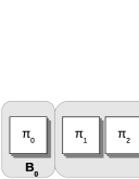
Figure 1: Example of a schedule divided into 4 blocks

Let $a$ and $b$ be the position of the first and last jobs of a block $B_{t}$ in the sequence, respectively, and let $b^{\prime}$ be the position of the last job of the predecessor block $B_{t-1}$ in the sequence with associated completion time $C\_b^{\prime}$. The cost of the block $B_{t}$, i.e., its total weighted tardiness, can be computed in $O(|B_{t}|$) steps as shown in Alg. 1. Note that if $|B_{t}|=1$, the procedure will not execute the loop from $a+1$ to $b$ described in lines 7-12 because in this case $a=b$ which implies in $b<a+1$.

Algorithm 1 CompCostBlock

1:Procedure CompCostBlock($b^{\prime},a,b,\pi,C\_b^{\prime}$)

2:$cost\leftarrow 0$

3:$Ctemp\leftarrow C\_b^{\prime}+s_{\pi_{b^{\prime}}\pi_{a}}+p_{\pi_{a}}$ $\triangleright$ Global variable that stores a temporary completion time

4:if $Ctemp>d_{\pi_{a}}$ then $\triangleright$ $d_{\pi_{a}}$ is the due date of job $\pi_{a}$

5:    $cost\leftarrow w_{\pi_{a}}\times(Ctemp-d_{\pi_{a}})$ $\triangleright$ $w_{\pi_{a}}$ is the weight of job $\pi_{a}$

6:end if

7:for $a^{\prime}=a+1\dots b$ do

8:    $Ctemp\leftarrow Ctemp+s_{\pi_{a^{\prime}-1}\pi_{a^{\prime}}}+p_{\pi_{a^{\prime}}}$

9:    if $Ctemp>d_{\pi_{a^{\prime}}}$ then

10:       $cost\leftarrow cost+w_{\pi_{a^{\prime}}}\times(Ctemp-d_{\pi_{a^{\prime}}})$

11:    end if

12:end for

13:return $cost$

14:end CompCostBlock.

It is easy to verify that the total cost of a sequence can be obtained by the sum of the costs of the blocks defined for that sequence. In the example given in Fig. 1 the total cost of the sequence is equal to the sum of the cost of blocks $B_{0}$, $B_{1}$, $B_{2}$ and $B_{3}$.

When performing move evaluations it is quite useful to define an auxiliary data structure that stores the cumulated weighted tardiness up to a certain position of the sequence. Therefore, we have decided to define an array $g$ for that purpose. For example, the element $g_{5}$ of the array stores the cumulated weighted tardiness up to the 5th position of the sequence.

We now proceed to a detailed description of the neighborhood structures used in our approach.

3.2.1 Swap

The swap neighborhood structure simply consists of exchanging the position of two jobs in the sequence, as depicted in Figure 2. It is possible to observe that the modified solution can be divided into 6 blocks. Alg. 2 shows how to compute the cost of a solution in $O(n-i)$ steps. Note that one can always assume that $i<j$ for every swap move.

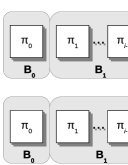
Figure 2: Exchanging the position of two jobs

Algorithm 2 CompCostSwap

1:Procedure CompCostSwap($\pi,i,j,g,C$)

2:$f\leftarrow g_{i-1}$ $\triangleright$ Variable that stores the cost to be evaluated

3:$Ctemp\leftarrow C_{\pi_{i-1}}$

4:$f\leftarrow f+\texttt{CompCostBlock}(i-1,j,j,\pi,Ctemp)$ $\triangleright$ Cost of block 4

5:$f\leftarrow f+\texttt{CompCostBlock}(j,i+1,j-1,\pi,Ctemp)$ $\triangleright$ Cost of block 3

6:$f\leftarrow f+\texttt{CompCostBlock}(j-1,i,i,\pi,Ctemp)$ $\triangleright$ Cost of block 2

7:$f\leftarrow f+\texttt{CompCostBlock}(i,j+1,n,\pi,Ctemp)$ $\triangleright$ Cost of block 5

8:return $f$

9:end CompCostSwap.

Alg. 3 presents the pseudocode of the neighborhood swap considering the limitation strategy described in Section 3.1. At first, the best sequence $\pi^{*}$ is considered to be the same as the original one, i.e., $\pi$ (line 2). Next, for every pair of positions $i$ and $j$ (with $j>i$) of $\pi$ (lines 3-17), the setup variation is computed in constant time (line 5). If this variation is smaller than or equal to $max\Delta s_{swap}$ (lines 7-15), then the cost of sequence $\pi^{\prime}$, which is a neighbor of $\pi$ generated by exchanging the position of customers $\pi_{i}$ and $\pi_{j}$, is computed using Alg. 2 (line 8). In case of improvement (lines 7-14), the best current solution is updated (line 10) and if the learning phase is activated, that is, if $max\Delta s_{swap}$ = $M$, list $\Delta s_{swap}$ is updated by adding the value associated to the setup variation computed in line 5 (lines 11-13). Finally, the procedure returns the best sequence $\pi^{*}$ found during the search (line 18).

Algorithm 3 Swap

1:Procedure Swap($\pi,g,C,\Delta s_{swap},max\Delta s_{swap}$)

2:$\pi^{*}\leftarrow\pi$; $f^{*}\leftarrow f(\pi)$;

3:for $i=1\dots n-1$ do

4:    for $j=i+1\dots n$ do

5:        $setupVariation=-s_{\pi_{i-1}\pi_{i}}-s_{\pi_{i}\pi_{i+1}}-s_{\pi_{j-1}\pi_{j}}-s_{\pi_{j}\pi_{j+1}}$

6:                                          $+s_{\pi_{i-1}\pi_{j}}+s_{\pi_{j}\pi_{i+1}}+s_{\pi_{j-1}\pi_{i}}+s_{\pi_{i}\pi_{j+1}}$

7:        if $setupVariation\leq max\Delta s_{swap}$ then

8:           $f(\pi^{\prime})$ = CompCostSwap($\pi$, $i$, $j$, $l$, $g$, $C$) $\triangleright$ $\pi^{\prime}$ is a neighbor of $\pi$

9:           if $f(\pi^{\prime})<f^{*}$ then

10:               $\pi^{*}\leftarrow\pi^{\prime}$; $f^{*}\leftarrow f(\pi^{\prime})$

11:               if $max\Delta s_{swap}$ = $M$ then $\triangleright$ Learning phase activated

12:                  $\Delta s_{swap}\leftarrow\Delta s_{swap}\cup setupVariation$

13:               end if

14:           end if

15:        end if

16:    end for

17:end for

18:return $\pi^{*}$;

19:end Swap.

3.2.2 $l$-block insertion

The $l$-block insertion neighborhood consists of moving a block of length $l$ forward ($i<j)$ or backward ($i>j$), as shown in Figs. 3 and 4, respectively. In this case the resulting solution in both cases can be represented by 5 blocks. Algs. 4 and 5 describe how to evaluate a cost of moving a block forward and backward in $O(n-i)$ and $O(n-j)$ steps, respectively.

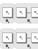
Figure 3: Forward insertion of a block of length $l$

Algorithm 4 CompCost$l$-blockF

1:Procedure CompCost$l$-blockF($\pi,i,j,l,g,C$)

2:$f\leftarrow g_{i-1}$ $\triangleright$ Variable that stores the cost to be evaluated

3:$Ctemp\leftarrow C_{\pi_{i-1}}$

4:$f\leftarrow f+\texttt{CompCostBlock}(i-1,i+l,j,\pi,Ctemp)$ $\triangleright$ Cost of block 3

5:$f\leftarrow f+\texttt{CompCostBlock}(j,i,i-1+l,\pi,Ctemp)$ $\triangleright$ Cost of block 2

6:$f\leftarrow f+\texttt{CompCostBlock}(i-1+l,j+1,n,\pi,Ctemp)$ $\triangleright$ Cost of block 4

7:return $f$

8:end CompCostF$l$-block.

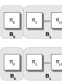
Figure 4: Backward insertion of a block of length $l$

Algorithm 5 CompCost$l$-blockB

1:Procedure CompCost$l$-blockB($\pi,i,j,l,g,C$)

2:$f\leftarrow g_{j-1}$ $\triangleright$ Variable that stores the cost to be evaluated

3:$Ctemp\leftarrow C_{\pi_{j-1}}$

4:$f\leftarrow f+\texttt{CompCostBlock}(j-1,i,i-1+l,\pi,Ctemp)$ $\triangleright$ Cost of block 3

5:$f\leftarrow f+\texttt{CompCostBlock}(i-1+l,j,i-1,\pi,Ctemp)$ $\triangleright$ Cost of block 2

6:$f\leftarrow f+\texttt{CompCostBlock}(i-1,i+l,n,\pi,Ctemp)$ $\triangleright$ Cost of block 4

7:return $f$

8:end CompCostB$l$-block.

It is worth mentioning that one can check at any time if the partial cost of the solution under evaluation is already worse than the best current cost. If so, the evaluation can be interrupted because it is already known that the solution under evaluation cannot be better than the current one. In some cases this may help speeding up the move evaluation process.

Let $L$ be a set composed of different values for the parameter $l$. In practice one can define a single neighborhood considering all values of $l\in L$ at once (see Xu et al. (2013)), or define multiple neighborhoods where each of them is associated with a given value of $l\in L$. In our implementation we decided for the latter option.

Alg. 6 shows the pseudocode of the neighborhood $l$-block taking into account the limitation strategy described earlier. This algorithm, which is divided into two parts, follows the same rationale of Alg. 3 in both of them. The main difference is related to the range of the positions $i$ and $j$, which depends on the value of $l$. In part one (lines 4-18) the search is performed forward, whereas in part 2 it is performed backward (lines 20-34).

Algorithm 6 $l$-blockInsertion

1:Procedure $l$-blockInsertion($\pi,l,g,C,\Delta s_{l\text{-}block},max\Delta s_{l\text{-}block}$)

2:$\pi^{*}\leftarrow\pi$; $f^{*}\leftarrow f(\pi)$;

3:$\triangleright$ Moving the $l$-block forward                                                                                                                     

4:for $i=1\dots n-l$ do

5:    for $j=i+1\dots n$ do

6:        $setupVariation=-s_{\pi_{i-1}\pi_{i}}-s_{\pi_{i-1+l}\pi_{i+l}}-s_{\pi_{j}\pi_{j+1}}$

7:                                          $+s_{\pi_{i-1}\pi_{i+l}}+s_{\pi_{j}\pi_{i}}+s_{\pi_{i-1+l}\pi_{j+1}}$

8:        if $setupVariation\leq max\Delta s_{l\text{-}block}$ then

9:           $f(\pi^{\prime})$ = CompCostl-blockF($\pi$, $i$, $j$, $l$, $g$, $C$) $\triangleright$ $\pi^{\prime}$ is a neighbor of $\pi$

10:           if $f(\pi^{\prime})<f^{*}$ then

11:               $\pi^{*}\leftarrow\pi^{\prime}$; $f^{*}\leftarrow f(\pi^{\prime})$

12:               if $max\Delta s_{l\text{-}block}$ = $M$ then $\triangleright$ Learning phase activated

13:                  $\Delta s_{l\text{-}block}\leftarrow\Delta s_{l\text{-}block}\cup setupVariation$;

14:               end if

15:           end if

16:        end if

17:    end for

18:end for

19:$\triangleright$ Moving the $l$-block backward                                                                                                                  

20:for $i=2\dots n-l+1$ do

21:    for $j=1\dots i-1$ do

22:        $setupVariation=-s_{\pi_{j-1}\pi_{j}}-s_{\pi_{i-1}\pi_{i}}-s_{\pi_{i-1+l}\pi_{i+1}}$

23:                                          $+s_{\pi_{j-1}\pi_{i}}+s_{\pi_{j-1+l}\pi_{j}}+s_{\pi_{i-1}\pi_{i+1}}$

24:        if $setupVariation\leq max\Delta s_{l\text{-}block}$ then

25:           $f(\pi^{\prime})$ = CompCostl-blockB($\pi$, $i$, $j$, $l$, $g$, $C$) $\triangleright$ $\pi^{\prime}$ is a neighbor of $\pi$

26:           if $f(\pi^{\prime})<f^{*}$ then

27:               $\pi^{*}\leftarrow\pi^{\prime}$; $f^{*}\leftarrow f(\pi^{\prime})$

28:               if $max\Delta s_{l\text{-}block}$ = $M$ then $\triangleright$ Learning phase activated

29:                  $\Delta s_{l\text{-}block}\leftarrow\Delta s_{l\text{-}block}\cup setupVariation$

30:               end if

31:           end if

32:        end if

33:    end for

34:end for

35:return $\pi^{*}$;

36:end $l$-blockInsertion.

3.3 Embedding the proposed approach in the ILS-RVND metaheuristic

In this section we explain how we embedded the proposed approach in the ILS-RVND metaheuristic (Subramanian, 2012). The reason for choosing this metaheuristic to test our local search limitation strategy is that it was found capable of generating highly competitive results not only for problem $1|s_{ij}|\sum w_{j}T_{j}$ (Subramanian et al., 2014), as mentioned in Section 2, but also for other combinatorial optimization problems (Subramanian et al., 2010; Subramanian, 2012; Silva et al., 2012; Penna et al., 2013; Subramanian and Battarra, 2013; Martinelli et al., 2013; Vidal et al., 2015). Moreover, the referred method relies on very few parameters and it can be considered relatively simple, which makes it quite practical and also easy to implement.

Alg. 7 highlights the differences between the original version of ILS-RVND and a new one, called ILS-RVND_Fast, that includes the additional steps (line 3 and lines 17-22) described in Section 3.1 for speeding up the the local search. It can be observed that the learning phase is limited to the first iteration of the algorithm, where the list $\Delta s_{v},\forall v\in\mathcal{N}$, is populated during the local search (line 9). The value of $max\Delta s_{v},\forall v\in\mathcal{N}$ is then estimated after the end of the first iteration. Parameters $I_{R}$ and $I_{ILS}$ correspond to the number of restarts of the metaheuristic and the number of consecutive ILS iterations without improvements, respectively. An exception occurs during the learning phase, which is more costly, where the number of ILS iterations is $I_{ILS}/2$. In both algorithms the initial solution (line 5) is generated using a simple randomized insertion heuristic, whereas the perturbation (line 14) is performed by a mechanism called double-bridge, which consists of exchanging two blocks of a sequence at random. The reader is referred to Subramanian et al. (2014) for implementation details about these procedures.

The local search method of both algorithms is performed by a RVND procedure, which consists of selecting an unexplored neighborhood at random whenever another one fails to find an improved solution. In case of improvement, all neighborhoods are reconsidered to be explored. Note that in both algorithms the set $L$ associated to the $l$-block neighborhood is provided as an input parameter to be tuned (see Section 4.1), as opposed to the ILS-RVND presented in Subramanian et al. (2014) where this set was predefined as $L=\{1,2,3\}$, that is, the $l$-block neighborhoods were limited to 1-, 2- and 3-block insertion. In addition, the neighborhood block reverse was also used in a restricted fashion by the authors, but it was not considered here because it did not seem to be crucial for obtaining high quality solutions.

One last remark is that the algorithm stops when a sequence $\pi$ with cost $f(\pi)=0$ is found. When this happens it is clear that an optimal solution was obtained and thus there is no point in continuing the search. This was not originally considered in the ILS-RVND presented in Subramanian et al. (2014), but it has been considered here in both versions.

Algorithm 7 ILS-RVND vs ILS-RVND_Fast

1:Procedure ILS-RVND($I_{R},I_{ILS},L$)

2:$f^{*}$ $\leftarrow$ $\infty$

3:

4:for $iter=1\dots I_{R}$ do

5:    $\pi\leftarrow\texttt{GenerateInitialSolution}()$

6:    $\hat{\pi}\leftarrow\pi$

7:    $iterILS\leftarrow 0$

8:    while $iterILS\leq I_{ILS}$ do

9:        $\pi\leftarrow\texttt{RVND}(\pi,L)$

10:        if $f(\pi)<f(\hat{\pi}$) then

11:           $\hat{\pi}\leftarrow\pi$

12:           $iterILS\leftarrow 0$

13:        end if

14:        $\pi\leftarrow\texttt{Perturb}(\hat{\pi})$

15:        $iterILS\leftarrow iterILS+1$

16:    end while

17:    

18:    

19:    

20:    

21:    

22:    

23:    if $f(\hat{\pi})<f^{*}$ then

24:        $\pi^{*}\leftarrow\hat{\pi}$; $f^{*}$ $\leftarrow$ $f(\hat{\pi})$

25:    end if

26:end for

27:return $\pi^{*}$

28:end ILS-RVND.

Procedure ILS-RVND_Fast($I_{R},I_{ILS},\theta,L$)

$f^{*}$ $\leftarrow$ $\infty$

$max\Delta s_{v}\leftarrow M;\Delta s_{v}\leftarrow\texttt{NULL},\forall v\in\mathcal{N}$

for $iter=1\dots I_{R}$ do

    $\pi\leftarrow\texttt{GenerateInitialSolution}()$

    $\hat{\pi}\leftarrow\pi$

    $iterILS\leftarrow 0$

    while $iterILS\leq I_{ILS}$ do $\triangleright$ or $iterILS\leq I_{ILS}/2$ when $iter=0$

        $\pi\leftarrow\texttt{RVND}(\pi,L,\Delta s,max\Delta s)$

        if $f(\pi)<f(\hat{\pi}$) then

           $\hat{\pi}\leftarrow\pi$

           $iterILS\leftarrow 0$

        end if

        $\pi\leftarrow\texttt{Perturb}(\hat{\pi})$

        $iterILS\leftarrow iterILS+1$

    end while

    if $iter=1$ then

        for $v=1\dots|\mathcal{N}|$ do

           $\Delta s_{v}\leftarrow$ sort($\Delta s_{v}$)

           $max\Delta s_{v}\leftarrow$ value associated to the position $\lfloor\theta\cdot|\Delta s_{v}|\rfloor$ of list $\Delta s_{v}$

        end for

    end if

    if $f(\hat{\pi})<f^{*}$ then

        $\pi^{*}\leftarrow\hat{\pi}$; $f^{*}$ $\leftarrow$ $f(\hat{\pi})$

    end if

end for

return $\pi^{*}$

end ILS-RVND_Fast.

4 Computational Experiments

The ILS-RVND and ILS-RVND_Fast algorithms were coded in C++ and the experiments were performed in an Intel Core i7 with 3.40 GHz and 16 GB of RAM running under Linux Mint 13. Only a single thread was used in our testing.

The 120 instances of Cicirello and Smith (2005) were used to evaluate the performance of the proposed algorithms. Each of them has 60 jobs and is characterized by three parameters: $\tau$, which is related to the tightness of the due date; $R$, which specifies the range of the due dates; $\eta$, which refers to the size of the average setup time with respect to the size of the average processing time. The authors created 12 groups of 10 instances by combining the following parameters: $\tau=\{0.3,0.6,0.9\}$, $R=\{0.25,0.75\}$ and $\eta=\{0.25,0.75\}$, as shown in Table 2.

Table 2: Group of instances generated by Cicirello and Smith (2005) for problem $1|s_{ij}|\sum w_{j}T_{j}$

Group	Instances	Configuration
1	1-10	$\tau=0.3,R=0.25,\eta=0.25$
2	11-20	$\tau=0.3,R=0.25,\eta=0.75$
3	21-30	$\tau=0.3,R=0.75,\eta=0.25$
4	31-40	$\tau=0.3,R=0.75,\eta=0.75$
5	41-50	$\tau=0.6,R=0.25,\eta=0.25$
6	51-60	$\tau=0.6,R=0.25,\eta=0.75$
7	61-70	$\tau=0.6,R=0.75,\eta=0.25$
8	71-80	$\tau=0.6,R=0.75,\eta=0.75$
9	81-90	$\tau=0.9,R=0.25,\eta=0.25$
10	91-100	$\tau=0.9,R=0.25,\eta=0.75$
11	101-110	$\tau=0.9,R=0.75,\eta=0.25$
12	111-120	$\tau=0.9,R=0.75,\eta=0.75$

4.1 Parameter Tuning

To have a better idea of the impact of the modifications introduced in the original ILS-RVND, we decided to use the same configuration for the number of ILS iterations as in Subramanian et al. (2014), that is, $I_{ILS}=4\times n$. However, since each iteration of the algorithm became much faster after implementing the limitation strategy (see Section 4.3) we decided to set $I_{R}=20$, instead of $I_{R}=10$, as in Subramanian et al. (2014), because it seemed to provide a better compromise between solution quality and computational time.

A set of 17 challenging instances was selected for tuning the parameters $L$ and $\theta$, namely instances 1, 2, 3, 4, 5, 7, 8. 9, 10, 11, 13, 14, 15, 16, 18, 20 and 24. The criterion used for choosing these instances was based on the difficulty faced by the ILS-RVND implemented in Subramanian et al. (2014) in finding their corresponding optimal solutions.

Let Best Gap be the gap between the best solution found in 10 runs and the optimal solution; Worst Gap be the gap between the worst solution found in 10 runs and the optimal solution; and Avg. Gap be the average gap between the average solution of 10 runs and the optimal solution. In the tables presented hereafter, Arithm. Mean of Best Gaps (%) corresponds to the arithmetic mean of the Best Gaps, Geom. Mean of Avg. Gaps (%) denotes the geometric mean of the Avg. Gaps, Geom. Mean of Worst Gaps (%) indicates the geometric mean of the Worst Gaps and Arithm. Mean of Avg. Time (s) is the arithmetic mean of the average times in seconds. Given a set of $q$ positive numbers, the geometric mean can be defined as the $q$th root of the product of all numbers of the set. The reason for using the geometric mean is because it normalizes the different ranges, that is, the possible significant differences among the Gaps. Hence, the geometric mean was adopted in some of the cases as an attempt to perform a fair comparison between the solutions found for each configuration tested. However, we used the arithmetic mean for the Best Gaps because in many cases the best solution found coincided with the optimal solution. In this case, the gap is equal to zero and thus the value is disregarded from the computation of the geometric mean, which may result in a misleading result when many values are not considered.

We have tested 34 different combination of neighborhoods, more precisely, we considered $L=\{1,\dots,4\}$ to $L=\{1,\dots,20\}$ incrementing one $l$-block neighborhood at a time and we tried each possibility with and without swap. Therefore, the goal of this experiment was not only to calibrate the parameter $L$, but also to investigate the benefits of including the neighborhood swap. For this testing, we have arbitrarily set $\theta=0.90$ and we ran the algorithm 10 times for each instance. Table 3 shows the average results obtained for the 17 instances mentioned above with the different combinations of neighborhoods. We decided to adopt the configuration $L=\{1,\dots,13\}$ + swap because it seemed to offer a good balance between solution quality and computational time.

Table 3: Results for the parameter tuning of $L$ with and without the neighborhood swap

	Arithm. Mean of	Geom. Mean of	Geom. Mean of	Arithm. Mean of
Neighborhoods	Best Gaps (%)	Avg. Gaps (%)	Worst Gaps (%)	Avg. Times (s)
$L=\{1,\dots,4\}$	2.95	2.94	5.02	6.44
$L=\{1,\dots,4\}$ + swap	3.23	2.76	4.93	6.12
$L=\{1,\dots,5\}$	2.29	2.07	4.12	6.66
$L=\{1,\dots,5\}$ + swap	2.43	1.94	3.22	6.96
$L=\{1,\dots,6\}$	1.95	1.44	3.01	7.66
$L=\{1,\dots,6\}$ + swap	1.44	1.38	2.95	7.51
$L=\{1,\dots,7\}$	1.07	1.13	2.60	15.58
$L=\{1,\dots,7\}$ + swap	1.72	1.07	2.05	7.95
$L=\{1,\dots,8\}$	0.82	1.16	2.61	12.75
$L=\{1,\dots,8\}$ + swap	2.05	1.18	1.98	8.22
$L=\{1,\dots,9\}$	1.42	1.09	2.21	10.11
$L=\{1,\dots,9\}$ + swap	1.24	0.90	1.68	8.68
$L=\{1,\dots,10\}$	1.92	0.91	1.79	10.96
$L=\{1,\dots,10\}$ + swap	1.11	0.79	1.74	9.23
$L=\{1,\dots,11\}$	1.05	1.00	1.84	12.15
$L=\{1,\dots,11\}$ + swap	0.75	0.88	1.70	9.72
$L=\{1,\dots,12\}$	0.30	0.79	1.64	9.47
$L=\{1,\dots,12\}$ + swap	0.51	0.79	1.70	9.73
$L=\{1,\dots,13\}$	1.06	0.80	1.94	10.02
L = {1,…,13} + swap	0.12	0.74	1.39	9.85
$L=\{1,\dots,14\}$	1.03	0.68	1.58	10.33
$L=\{1,\dots,14\}$ + swap	0.39	0.84	1.69	10.24
$L=\{1,\dots,15\}$	1.15	0.78	1.66	10.40
$L=\{1,\dots,15\}$ + swap	1.35	0.71	1.49	10.42
$L=\{1,\dots,16\}$	1.01	0.89	1.81	10.70
$L=\{1,\dots,16\}$ + swap	0.31	0.70	1.49	11.00
$L=\{1,\dots,17\}$	0.81	0.78	1.56	11.29
$L=\{1,\dots,17\}$ + swap	0.75	0.80	1.52	11.39
$L=\{1,\dots,18\}$	0.83	0.77	1.60	11.72
$L=\{1,\dots,18\}$ + swap	0.31	0.71	1.57	11.63
$L=\{1,\dots,19\}$	0.13	0.74	1.53	11.74
$L=\{1,\dots,19\}$ + swap	0.90	0.90	1.83	11.81
$L=\{1,\dots,20\}$	1.32	0.93	1.72	12.16
$L=\{1,\dots,20\}$ + swap	1.07	0.74	1.41	11.94

Five different values for the parameter $\theta$ was tested, in particular, 0,80, 0.85, 0.90, 0.95 and 1.00, and the results can be found in Table 4. As expected, it can be observed that the average computational time is directly proportional to $\theta$ since more moves are considered for evaluation as the value of $\theta$ increases. Note that $\theta=1.00$ implies that $max\Delta s_{v}$ is equal to the largest setup variation associated to an improving move of neighborhood $v\in\mathcal{N}$ that occurred during the learning phase. We decided to adopt $\theta=0.90$ because solutions of similar quality were obtained when compared to $\theta=1.00$, but approximately four times faster.

Table 4: Results for the parameter tuning of $\theta$

	Arithm. Mean of	Geom. Mean of	Geom. Mean of	Arithm. Mean of
$\theta$	Best Gaps (%)	Avg. Gaps (%)	Worst Gaps (%)	Avg. Times (s)
0.80	0.15	0.97	2.05	7.44
0.85	1.25	0.78	1.56	8.11
0.90	1.11	0.75	1.59	10.12
0.95	1.51	0.66	1.34	16.81
1.00	0.91	0.74	1.70	41.74

4.2 Comparison with the literature

In this section we compare the best, average and worst results found by ILS-RVND_Fast over 10 runs with the best methods available in the literature. We specify below the algorithms considered for comparison as well as the type of result reported by the associated work.

ACO${}_{\text{AP}}$: Ant Colony Optimization of Anghinolfi and Paolucci (2008). Best of 10 runs.

DPSO: Discrete Particle Swarm Optimization of Anghinolfi and Paolucci (2009). Best of 10 runs.

DDE: Discrete Differential Evolutionary heuristic of Tasgetiren et al. (2009). Best of 10 runs.

GVNS: General Variable Neighborhood Search of Kirlik and Oğuz (2012). Best of 20 runs.

ILS${}_{\text{XLC}}$: Iterated Local Search of Xu et al. (2013). Best and average of 100 runs.

ILS-RVND${}_{\text{SBP}}$: Iterated Local Search + Randomized Variable Neighborhood Descent of Subramanian et al. (2014). Best and average of 10 runs.

LOX$\oplus$B: Hybrid Evolutionary Algorithm of Xu et al. (2014). Best and average of 20 runs.

Opt: Optimal solution found by the exact algorithm of Tanaka and Araki (2013).

Table LABEL:Comparison presents the results found by ILS-RVND_Fast and also by the algorithms mentioned above, except ACO${}_{\text{AP}}$ for space restriction reasons. The average times reported in this table are in seconds. It can be observed that the proposed algorithm was capable of finding the optimal solution for all instances, except for instance 24. Moreover, it is possible to verify that the mean of the average times of ILS-RVND_Fast was approximately 13 seconds.

Table 5: Results for the instances of Cicirello and Smith (2005)

		DPSO		DDE		GVNS		ILS${}_{\text{XLC}}\!\!\!$			ILS-RVND${}_{\text{SBP}}\!\!\!$			LOX$\oplus$B			ILS-RVND${}_{Fast}\!\!\!$
Inst	Opt																			Avg.
		Best		Best		Best		Best	Avg.		Best	Avg.		Best	Avg.		Best	Avg.	Worst	Time
1	453	531		474		471		453	480.3		459	470.4		453	462.2		453	457.5	459	8.5
2	4794	5088		4902		4878		4794	4887.0		4866	4910.4		4794	4841.5		4794	4813.8	4842	11.1
3	1390	1609		1465		1430		1390	1457.5		1414	1433.9		1390	1401.8		1390	1393	1395	10.8
4	5866	6146		5946		6006		5866	5978.4		5906	5982		5866	5871.2		5866	5866	5866	7.0
5	4054	4339		4084		4114		4074	4215.9		4084	4129		4054	4096.9		4054	4072	4084	10.9
6	6592	6832		6652		6667		6592	6750.3		6607	6665.5		6592	6617.2		6592	6593.5	6607	9.1
7	3267	3514		3350		3330		3267	3404.2		3350	3394.2		3267	3319.0		3267	3281.2	3296	14.2
8	100	132		114		108		100	106.2		105	109.6		100	102.1		100	101	102	7.7
9	5660	6153		5803		5751		5660	5840.8		5673	5760.1		5660	5699.5		5660	5665.2	5673	11.3
10	1740	1895		1799		1789		1740	1793.0		1768	1783.5		1740	1756.8		1740	1746.3	1761	9.3
11	2785	3649		3294		2998		2830	3125.0		2934	3062.8		2798	2871.0		2785	2858.1	2894	8.19
12	0	0		0		0		0	0.0		0	0		0	0.0		0	0	0	$<0.1$
13	3904	4430		4194		4068		3942	4141.9		4014	4103.1		3904	3986.5		3904	3949.0	3978	7.86
14	2075	2749		2268		2260		2081	2315.1		2219	2279.4		2075	2179.3		2075	2128.2	2174	9.45
15	724	1250		964		935		775	891.3		896	953.6		724	794.8		724	771	809	7.1
16	3285	4127		3876		3381		3285	3413.5		3325	3415.3		3285	3306.6		3285	3296.2	3301	9.3
17	0	75		61		0		0	13.6		0	31.1		0	2.5		0	0	0	1.2
18	767	971		857		845		767	813.5		787	812.5		767	789.0		767	776.4	789	8.6
19	0	0		0		0		0	0.0		0	0		0	0.0		0	0	0	$<0.1$
20	1757	2675		2111		2053		1757	1938.9		1789	1920.2		1757	1790.9		1757	1757.8	1761	7.5
21	0	0		0		0		0	0.0		0	0		0	0.0		0	0	0	$<0.1$
22	0	0		0		0		0	0.0		0	0		0	0.0		0	0	0	$<0.1$
23	0	0		0		0		0	0.0		0	0		0	0.0		0	0	0	$<0.1$
24	761	1043		1033		920		773	1037.2		1004	1028		761	1027.8		773	967.9	1030	24.5
25	0	0		0		0		0	0.0		0	0		0	0.0		0	0	0	$<0.1$
26	0	0		0		0		0	0.0		0	0		0	0.0		0	0	0	$<0.1$
27	0	0		0		0		0	0.0		0	0		0	0.0		0	0	0	0.2
28	0	0		0		0		0	0.0		0	0		0	0.0		0	0	0	$<0.1$
29	0	0		0		0		0	0.0		0	0		0	0.0		0	0	0	$<0.1$
30	0	0		0		0		0	28.2		0	0		0	24.9		0	0	0	0.2
31	0	0		0		0		0	0.0		0	0		0	0.0		0	0	0	$<0.1$
32	0	0		0		0		0	0.0		0	0		0	0.0		0	0	0	$<0.1$
33	0	0		0		0		0	0.0		0	0		0	0.0		0	0	0	$<0.1$
34	0	0		0		0		0	0.0		0	0		0	0.0		0	0	0	$<0.1$
35	0	0		0		0		0	0.0		0	0		0	0.0		0	0	0	$<0.1$
36	0	0		0		0		0	0.0		0	0		0	0.0		0	0	0	$<0.1$
37	0	186		107		46		0	293.3		0	119		0	77.4		0	18.0	56	16.8
38	0	0		0		0		0	0.0		0	0		0	0.0		0	0	0	$<0.1$
39	0	0		0		0		0	0.0		0	0		0	0.0		0	0	0	$<0.1$
40	0	0		0		0		0	0.0		0	0		0	0.0		0	0	0	$<0.1$
41	69102	69102		69242		69242		69102	69318.2		69102	69200		69102	69222.7		69102	69102	69102	21.2
42	57487	57487		57511		57511		57487	57644.6		57487	57489.4		57487	57558.0		57487	57487	57487	17.5
43	145310	145883		145310		145310		145310	145930.5		145310	145771.7		145310	145659.6		145310	145370	145794	15.3
44	35166	35331		35289		35289		35166	35328.3		35166	35251.4		35166	35253.8		35166	35166	35166	13.0
45	58935	59175		58935		59025		58935	59018.6		58935	58944		58935	58974.6		58935	58935	58935	19.7
46	34764	34805		34764		34764		34764	35034.8		34764	34817.3		34764	34896.8		34764	34764	34764	18.6
47	72853	73378		73005		72853		72853	73160.4		72853	73028		72853	73070.6		72853	72853	72853	16.6
48	64612	64612		64612		64612		64612	64719.6		64612	64638.9		64612	64699.6		64612	64612	64612	30.2
49	77449	77771		77641		77833		77449	78176.6		77449	77794.2		77449	78091.2		77449	77449	77449	15.4
50	31092	31810		31565		31292		31092	31580.6		31092	31359.8		31092	31194.6		31092	31092	31092	17.0
51	49208	49907		49927		49761		49208	50082.5		49208	49638.3		49208	49510.6		49208	49373.2	49621	8.2
52	93045	94175		94603		93106		93045	94653.3		93045	93722.2		93045	93782.8		93045	93045	93045	15.5
53	84841	86891		84841		84841		84841	86465.3		84841	85422.4		84841	86566.7		84841	84841	84841	13.5
54	118809	118809		119226		119074		118809	120150.8		118809	119194.9		118809	119639.6		118809	118872	119117	11.7
55	64315	68649		66006		65400		64315	66055.4		64315	65240.2		64315	65106.7		64315	64315	64315	12.8
56	74889	75490		75367		74940		74889	75472.9		74889	75038.9		74889	75060.2		74889	74894.1	74940	13.8
57	63514	64575		64552		64575		63514	65195.4		63514	64195.4		63514	64494.3		63514	63593.2	64306	9.5
58	45322	45680		45322		45322		45322	46286.1		45322	45495.2		45322	45781.0		45322	45322	45322	11.1
59	50999	52001		52207		51649		50999	51954.0		50999	51463.4		50999	51348.2		50999	51162.8	51233	10.9
60	60765	63342		60765		61755		60765	62498.8		60765	61843.8		60765	61397.4		60765	60866.7	61782	7.7
61	75916	75916		75916		75916		75916	75998.5		75916	75916		75916	76094.9		75916	75916	75916	28.8
62	44769	44769		44769		44769		44769	44840.0		44769	44775		44769	44833.1		44769	44769	44769	24.7
63	75317	75317		75317		75317		75317	75536.9		75317	75317		75317	75627.0		75317	75317	75317	27.1
64	92572	92572		92572		92572		92572	92609.8		92572	92572		92572	92650.5		92572	92572	92572	23.1
65	126696	126696		126696		126696		126696	127080.1		126696	126696		126696	127428.5		126696	126696	126696	27.5
66	59685	59685		59685		59685		59685	59927.3		59685	59685		59685	60034.8		59685	59685	59685	32.0
67	29390	29390		29390		29390		29390	29415.8		29390	29390.4		29390	29397.0		29390	29390	29390	21.9
68	22120	22120		22120		22120		22120	22264.6		22120	22159.2		22120	22143.0		22120	22120	22120	26.3
69	71118	71118		71118		71118		71118	71307.7		71118	71118		71118	71164.6		71118	71118	71118	23.8
70	75102	75102		75102		75102		75102	75427.4		75102	75123		75102	75433.9		75102	75102	75102	26.5
71	145007	145771		145007		145007		145007	147119.7		145007	145561.2		145007	146653.5		145007	145272	146121	21.3
72	43286	43994		43904		43286		43286	45678.3		43286	43706.4		43286	44177.7		43286	43286	43286	18.7
73	28785	28785		28785		28785		28785	29054.4		28785	28803.8		28785	29129.3		28785	28785	28785	18.1
74	29777	30734		30313		30136		29777	30765.0		29777	30248		29777	30378.2		29777	29777	29777	15.0
75	21602	21602		21602		21602		21602	22450.0		21602	21790.8		21602	22130.9		21602	21617.6	21758	15.2
76	53555	53899		53555		54024		53555	54529.2		53555	53752.2		53555	53819.2		53555	53717.6	54024	13.9
77	31817	31937		32237		31817		31937	33374.4		31817	32126.4		31817	32797.0		31817	31973.6	32237	21.2
78	19462	19660		19462		19462		19462	20381.8		19462	19481.8		19462	19871.3		19462	19481.8	19660	11.2
79	114999	114999		114999		114999		114999	116196.8		114999	114999		114999	116054.9		114999	114999	114999	14.5
80	18157	18157		18157		18157		18157	19274.4		18157	18300.7		18157	18660.2		18157	18157	18157	13.6
81	383485	383703		383485		383485		383485	383903.1		383485	383485		383485	383662.7		383485	383485	383485	13.3
82	409479	409544		409544		409479		409479	409815.6		409479	409544		409479	409922.4		409479	409486	409544	20.5
83	458752	458787		458752		458752		458752	458922.1		458752	458771.8		458752	458980.5		458752	458756	458787	23.1
84	329670	329670		329670		329670		329670	329969.7		329670	329800.5		329670	329978.1		329670	329675	329720	19.2
85	554766	555130		554993		554766		554766	555107.2		554766	554822		554766	555118.6		554766	554771	554773	25.6
86	361417	361417		361417		361417		361417	361826.3		361417	361417		361417	361576.4		361417	361417	361417	20.1
87	398551	398551		398670		398551		398551	398623.8		398551	398562.9		398551	398645.1		398551	398551	398551	17.3
88	433186	433519		433186		433244		433186	433564.4		433186	433235.6		433186	433463.8		433186	433219	433244	22.7
89	410092	410092		410092		410092		410092	410187.3		410092	410092		410092	410411.9		410092	410092	410092	18.1
90	401653	401653		401653		401653		401653	401825.5		401653	401663.2		401653	401843.7		401653	401653	401653	17.4
91	339933	343029		340508		339933		339933	340079.3		339933	339961.8		339933	340025.4		339933	339933	339933	27.0
92	361152	361152		361152		361152		361152	362030.6		361152	361399.5		361152	362196.9		361152	361152	361152	8.6
93	403423	406728		404548		404917		403423	405344.0		403423	404407.6		403423	404958.1		403423	403456	403757	11.5
94	332941	332983		333020		332949		332941	333319.3		332949	332979.7		332941	333178.9		332941	332968	333020	7.6
95	516926	521208		517011		517646		516926	518751.3		516926	517316.5		516926	518849.9		516926	517115	517398	11.0
96	455448	459321		457631		457631		455448	457814.4		455448	456178.1		455448	458241.3		455448	455650	457249	12.0
97	407590	410889		409263		407590		407590	408437.8		407590	407590		407590	408981.6		407590	407590	407590	12.0
98	520582	522630		523486		520582		520582	522055.2		520582	521145.8		520582	522093.9		520582	520582	520582	14.1
99	363518	365149		364442		363977		363518	364803.2		363518	364000.7		363518	364709.5		363518	363728	363977	10.7
100	431736	432714		431736		432068		431736	433105.8		432068	432396		431736	432781.5		431736	431736	431736	10.8
101	352990	352990		352990		352990		352990	353033.1		352990	352990		352990	353004.9		352990	352990	352990	17.8
102	492572	493069		492748		492572		492572	492832.6		492572	492572		492572	492914.3		492572	492572	492572	14.2
103	378602	378602		378602		378602		378602	378834.0		378602	378602		378602	378934.1		378602	378602	378602	15.0
104	357963	357963		357963		357963		357963	358174.6		357963	357995.6		357963	358077.2		357963	357968	358017	18.2
105	450806	450806		450806		450806		450806	450812.4		450806	450806.2		450806	450889.9		450806	450806	450806	19.1
106	454379	455152		454379		454379		454379	454851.6		454379	454379		454379	455091.8		454379	454379	454379	22.5
107	352766	352867		352766		352766		352766	353002.3		352766	352826.2		352766	353153.6		352766	352766	352766	18.1
108	460793	460793		460793		460793		460793	461112.6		460793	460793		460793	461390.3		460793	460793	460793	28.7
109	413004	413004		413004		413004		413004	413426.1		413004	413130.2		413004	413643.8		413004	413006	413019	16.9
110	418769	418769		418769		418769		418769	419030.4		418769	418834.2		418769	418954.5		418769	418769	418769	13.4
111	342752	342752		342752		342752		342752	343768.0		342752	342805.2		342752	343687.6		342752	342752	342752	17.4
112	367110	369237		367110		367110		367110	369592.0		367110	367970.4		367110	368861.7		367110	367110	367110	17.6
113	259649	260176		260872		259649		259649	259909.2		259649	259676.9		259649	260246.4		259649	259649	259649	9.6
114	463474	464136		465503		463474		463474	465440.2		463474	464377.1		463474	465440.2		463474	463508	463813	8.4
115	456890	457874		457289		457189		456890	458414.7		456890	457046.1		456890	458414.7		456890	456923	457189	17.0
116	530601	532456		530803		530601		530601	531410.8		530601	530614.4		530601	531410.8		530601	530601	530601	10.9
117	502840	503199		502840		503046		502840	503600.9		502840	502991.5		502840	503600.9		502840	502840	502840	13.8
118	349749	350729		349749		349749		349749	352050.9		349749	350326.2		349749	352050.9		349749	349749	349749	15.5
119	573046	573046		573046		573046		573046	573759.3		573046	573122.1		573046	573759.3		573046	573046	573046	12.0
120	396183	396183		396183		396183		396183	398005.1		396183	396592.5		396183	398005.1		396183	396183	396183	15.4
																			Mean	13.07

Table 5: (Continued)

Table 6 presents a summary of the results found by ILS-RVND_Fast compared with those achieved by several heuristics from the literature. A direct comparison with some of the algorithms such as ACO${}_{\text{AP}}$, DPSO, DDE and GVNS becomes quite hard because the average results were not reported by the authors. With respect to the best solutions, our algorithm clearly outperforms these four by a good margin. Even our average and worst solutions are, in most cases, better or equal than the best ones of such methods.

The average and worst solutions of ILS-RVND_Fast are always equal or better than the average solutions of ILS${}_{\text{XLC}}$. The same happened to ILS-RVND${}_{\text{SBP}}$ and LOX$\oplus$B, except for few cases where the worst solutions of ILS-RVND_Fast were not better than the average solution of these two methods. Worst solutions were only reported for ILS-RVND${}_{\text{SBP}}$, where all them are either equal or worse than those of ILS-RVND_Fast. The results suggest that our algorithm is very competitive in terms of solution quality.

Table 6: Summary of the results found by ILS-RVND_Fast compared to several heuristic methods from the literature

	ACO${}_{\text{AP}}$	DPSO	DDE	GVNS	ILS${}_{\text{XLC}}$	ILS-RVND${}_{\text{SBP}}$	LOX$\oplus$B
$\#Best$ improved	84	66	52	44	6	20	1
$\#Best$ equaled	36	54	68	76	114	100	118
$\#Best$ worse	0	0	0	0	0	0	1
$\#Avg.$ better than the Best	84	65	51	42	2	19	0
$\#Avg.$ equal to the Best	34	49	57	64	76	74	76
$\#Avg.$ improved	–	–	–	–	101	83	101
$\#Avg.$ equaled	–	–	–	–	19	37	19
$\#Avg.$ worse	–	–	–	–	0	0	0
$\#Worst$ better than the Best	82	59	47	34	0	13	0
$\#Worst$ equal to the Best	34	52	51	69	76	78	76
$\#Worst$ better than the Avg.	–	–	–	–	101	69	91
$\#Worst$ equal to the Avg.	–	–	–	–	19	37	20
$\#Worst$ improved	–	–	–	–	–	82	–
$\#Worst$ equaled	–	–	–	–	–	38	–
$\#Worst$ worse	–	–	–	–	–	0	–

Table 7 shows the time in seconds spent by ILS-RVND_Fast to find or improve the solutions found by the algorithms that were chosen for comparison. In this case the stopping criterion no longer depends on the number of restarts, but on a target value from the literature. The algorithm was executed 10 times for each instance and we report the mean (arithmetic), median, minimum and maximum of the average times by group required to find or improve the target value. We also report the average values considering all instances at once (last column of the table).

Table 7: Average time in seconds required by ILS-RVND_Fast to find or improve the solutions found by different algorithms from the literature

			Group
			1	2	3	4	5	6	7	8	9	10	11	12	All
ACO${}_{\text{AP}}$	Best	Mean	0.5	0.2	0.2	0.2	1.2	1.0	2.9	3.4	7.2	2.2	2.9	1.7	2.0
		Median	0.3	0.1	$<0.1$	$<0.1$	0.7	0.9	2.7	1.8	1.9	1.1	2.3	1.5	0.9
		Min	0.3	$<0.1$	$<0.1$	$<0.1$	0.2	0.5	0.4	0.7	0.4	0.5	0.3	0.3	$<0.1$
		Max	1.6	0.7	1.2	1.7	3.5	1.5	5.5	12.3	47.2	11.6	6.7	4.5	47.2
DPSO	Best	Mean	0.6	0.3	0.4	0.4	3.1	2.8	5.1	7.5	3.8	2.2	3.7	3.3	2.8
		Median	0.4	0.3	$<0.1$	$<0.1$	2.8	2.1	3.9	6.7	2.9	1.8	2.9	3.3	2.2
		Min	0.2	$<0.1$	$<0.1$	$<0.1$	0.9	0.4	2.2	3.3	1.9	0.3	0.7	0.1	$<0.1$
		Max	1.3	1.1	2.3	3.7	9.6	8.7	15.3	15.5	8.1	6.3	7.9	6.0	15.5
DDE	Best	Mean	2.1	0.7	1.0	0.5	4.9	3.9	5.5	9.0	12.5	5.2	5.8	4.5	4.6
		Median	1.6	0.4	$<0.1$	$<0.1$	3.8	4.0	3.1	8.0	4.6	3.3	5.4	4.4	3.0
		Min	1.3	$<0.1$	$<0.1$	$<0.1$	0.9	1.6	0.8	3.4	1.0	1.0	1.6	0.9	$<0.1$
		Max	7.3	2.7	7.9	5.1	15.5	6.9	21.3	22.3	81.8	23.9	12.9	8.7	81.8
GVNS	Best	Mean	2.3	1.4	11.4	1.0	3.6	5.2	5.8	15.0	14.9	4.0	4.7	4.8	6.2
		Median	2.2	1.4	$<0.1$	$<0.1$	2.6	5.3	4.1	6.3	5.8	3.5	3.5	3.8	3.1
		Min	0.6	$<0.1$	$<0.1$	$<0.1$	0.8	2.8	1.6	3.0	2.8	2.6	1.9	2.1	$<0.1$
		Max	4.4	3.0	113.1	9.9	8.1	8.1	15.4	82.9	81.3	10.1	11.9	8.6	113.1
ILS${}_{\text{XLC}}$	Best	Mean	21.4	17.0	282.21	5.5	6.0	8.3	3.8	9.2	14.8	11.1	4.2	8.3	32.62
		Median	17.8	8.1	$<0.1$	$<0.1$	5.2	8.0	3.0	7.5	6.5	5.6	3.9	4.2	4.9
		Min	2.3	$<0.1$	$<0.1$	$<0.1$	1.6	4.2	1.8	2.9	1.0	2.0	1.7	2.2	$<0.1$
		Max	54.6	47.9	2820.4	54.8	13.4	13.7	8.8	17.0	52.1	32.6	8.6	42.0	2820.4
	Avg	Mean	1.5	1.6	0.3	0.4	2.4	2.1	2.5	2.6	2.8	2.6	1.9	2.5	1.9
		Median	1.3	1.8	$<0.1$	$<0.1$	1.8	2.2	2.1	2.6	2.4	2.7	1.6	2.3	1.9
		Min	0.9	$<0.1$	$<0.1$	$<0.1$	1.3	0.9	1.7	1.0	1.6	1.3	0.7	0.9	$<0.1$
		Max	3.0	2.6	2.4	4.4	4.1	3.1	4.1	5.2	5.3	4.8	4.5	4.0	5.3
ILS-RVND${}_{\text{SBP}}$	Best	Mean	4.1	2.6	5.3	4.3	5.5	11.4	4.6	17.1	18.4	9.3	5.2	7.1	7.9
		Median	3.2	2.9	$<0.1$	$<0.1$	5.6	10.5	3.0	8.3	5.0	4.9	4.6	4.7	4.1
		Min	1.7	$<0.1$	$<0.1$	$<0.1$	2.2	5.7	1.4	3.4	1.6	2.9	1.8	3.0	$<0.1$
		Max	7.3	5.2	52.0	43.2	8.7	25.6	19.3	88.6	67.7	35.7	14.4	29.8	88.6
	Avg	Mean	1.9	1.6	1.5	0.6	4.1	5.0	4.2	8.0	8.5	5.7	3.7	4.0	4.1
		Median	2.0	1.8	$<0.1$	$<0.1$	3.4	5.3	4.2	7.3	4.3	3.7	3.8	3.8	3.2
		Min	1.3	$<0.1$	$<0.1$	$<0.1$	2.0	2.6	1.2	5.0	1.4	2.3	1.4	0.6	$<0.1$
		Max	2.5	3.1	14.1	5.5	9.4	6.5	8.1	16.7	41.8	24.4	7.6	9.6	41.8
LOX$\oplus$B	Best	Mean	48.1	87.6	1685.83	5.5	6.0	8.3	3.8	15.8	14.8	11.1	4.2	8.3	158.34
		Median	21.0	28.9	$<0.1$	$<0.1$	5.2	8.0	3.0	7.5	6.5	5.6	3.9	4.2	4.9
		Min	2.3	$<0.1$	$<0.1$	$<0.1$	1.6	4.2	1.8	2.9	1.0	1.9	1.7	2.2	$<0.1$
		Max	281.3	318.5	16856.4	54.8	13.4	13.7	8.8	82.9	52.1	32.6	8.6	42.0	16856.4
	Avg	Mean	4.0	3.3	2.2	0.6	3.9	4.7	2.4	5.6	2.6	2.2	1.7	2.6	3.0
		Median	3.5	3.5	$<0.1$	$<0.1$	3.4	4.8	2.5	4.7	2.8	2.2	1.5	1.8	2.4
		Min	2.8	$<0.1$	$<0.1$	$<0.1$	1.8	1.4	0.9	1.9	0.5	1.5	0.5	0.5	$<0.1$
		Max	7.6	6.6	20.0	5.6	7.9	10.3	4.7	11.8	4.5	3.8	4.2	8.4	20.0
Optimal		Mean	48.1	122.9	1685.83	5.5	6.0	8.3	3.8	15.8	14.8	11.1	4.2	8.3	161.25
		Median	21.0	28.9	0.01	$<0.1$	5.2	8.0	3.0	7.5	6.5	5.6	3.9	4.2	4.9
		Min	2.3	$<0.1$	$<0.1$	$<0.1$	1.6	4.2	1.8	2.9	1.0	2.0	1.7	2.2	$<0.1$
		Max	281.3	605.0	16856.4	54.8	13.4	13.7	8.8	82.9	52.1	32.6	8.6	42.0	16856.4
1: 0.1 seconds disregarding instance 24
2: 9.2 seconds disregarding instance 24
3: 0.2 seconds disregarding instance 24
4: 18.0 seconds disregarding instance 24
5: 20.9 seconds disregarding instance 24

On one hand, it can be observed from Table 7 that ILS-RVND_Fast was capable of finding or improving the best solutions of ACO${}_{\text{AP}}$, DPSO, DDE, GVNS and ILS-RVND${}_{\text{SBP}}$ in only 2.0, 2.8, 4.6, 6.2 and 7.9 seconds, on average, respectively. On the other hand, ILS-RVND_Fast spent, on average, 32.6, 158.3 and 161.2 seconds to find or improve the best solutions of ILS${}_{\text{XLC}}$, LOX$\oplus$B and the optimal solutions, respectively. However, if we disregard instance 24, these values significantly decrease to 9.2, 18.0 and 20.9 seconds, respectively.

Moreover, ILS-RVND_Fast found or improved the average solutions of ILS${}_{\text{XLC}}$, ILS-RVND${}_{\text{SBP}}$ and LOX$\oplus$B in only 1.9, 4.1 and 3.0 seconds, respectively, on average. It is worth mentioning that the average solutions of ILS${}_{\text{XLC}}$ in Xu et al. (2013) and LOX$\oplus$B in Xu et al. (2014) were obtained in 100 seconds on an Intel Core i3 3.10 GHz with 2.0 GB of RAM, whereas the average solutions of ILS-RVND${}_{\text{SBP}}$ were obtained in 23.4 seconds on an Intel Core i5 3.20 GHz with 4.0 GB of RAM. The hardware configuration of these two machines is slightly inferior than the one used in our experiments (Intel Core i7 with 3.40 GHz and 16 GB of RAM), and thus does not justify the considerable difference in terms of CPU time between ILS-RVND_Fast and the three other methods. Therefore, from Tables LABEL:Comparison-7, we can conclude that ILS-RVND_Fast is, on average, remarkably faster and clearly more efficient than those three heuristic algorithms, which are the best ones available in the literature for problem $1|s_{ij}|\sum w_{j}T_{j}$.

4.3 Impact of the proposed local search limitation strategy

In this section we investigate the effect of the proposed local search limitation strategy on the performance of the algorithm. We start by analyzing the average percentage of moves that were not evaluated per neighborhood in all groups of instances, as shown in Table 8. It can be verified that the proportion of moves that were not considered for evaluation varied according to the characteristics of the group, ranging, on average, from 69.6% (Group 7) to 98.8% (Group 2).

Table 8: Average percentage of moves that were not evaluated

	Group
Neighborhoods	1	2	3	4	5	6	7	8	9	10	11	12
1-block insertion	87.7	96.2	89.4	94.9	81.7	93.9	78.5	91.6	89.3	94.5	88.5	94.9
2-block insertion	92.7	96.9	90.9	96.7	82.2	93.7	75.2	90.0	84.6	93.1	83.4	93.9
3-block insertion	95.0	97.9	91.4	96.6	82.0	93.6	73.7	89.8	80.3	91.8	78.8	92.6
4-block insertion	96.4	99.0	86.3	96.4	85.5	94.9	74.6	90.9	80.1	91.8	78.1	92.3
5-block insertion	96.6	99.5	86.7	97.1	83.7	95.6	73.3	91.1	80.7	91.0	78.9	92.5
6-block insertion	96.8	99.6	79.0	95.5	85.8	95.0	75.2	91.1	81.9	90.7	79.5	91.8
7-block insertion	97.5	99.5	78.7	95.5	84.1	95.1	72.6	89.8	81.7	91.0	79.0	92.4
8-block insertion	97.5	99.5	79.1	96.5	83.4	93.9	69.3	89.0	78.9	90.4	75.7	92.0
9-block insertion	96.5	99.5	79.4	94.0	80.4	94.0	65.1	87.5	77.7	90.6	74.8	90.2
10-block insertion	96.7	99.6	83.4	94.7	79.0	92.9	63.9	85.7	75.2	88.9	71.2	89.5
11-block insertion	96.4	99.4	79.1	94.9	76.7	92.5	61.4	84.5	71.3	87.3	69.8	89.1
12-block insertion	96.2	99.5	71.5	92.1	74.7	91.4	58.3	83.9	69.4	86.8	66.5	87.6
13-block insertion	94.9	99.3	72.7	92.8	72.4	90.4	55.0	82.6	67.0	86.2	63.5	86.0
Swap	89.7	98.3	87.3	96.8	81.7	95.4	78.0	92.5	90.1	94.8	89.7	95.7
Mean	95.0	98.8	82.5	95.3	80.9	93.7	69.6	88.6	79.1	90.6	77.0	91.5

Since a very large number of moves were not considered for evaluation, we decided to conduct an experiment to verify the level of accuracy of the limitation strategy. Table 9 shows, for each neighborhood and for each group, the average percentage of improving moves that were not evaluated, here denoted as lost improving moves. We can observe that the average percentage of lost improving moves was relatively small in all cases (never more than 11%), thus ratifying the effectiveness of the proposed limitation strategy.

Table 9: Average percentage of improving moves that were not evaluated

	Group
Neighborhoods	1	2	3	4	5	6	7	8	9	10	11	12
1-block insertion	10.9	8.2	1.8	2.3	9.4	10.0	10.0	9.6	9.6	9.7	9.7	9.6
2-block insertion	10.0	8.7	1.3	1.0	9.9	9.6	9.8	9.9	10.0	10.0	9.8	9.7
3-block insertion	9.9	8.8	2.8	2.9	9.3	9.9	9.9	9.6	9.7	10.4	9.6	9.7
4-block insertion	9.9	7.8	2.6	1.2	9.8	9.9	9.6	9.4	9.9	10.0	9.8	10.0
5-block insertion	9.8	7.8	1.3	1.2	9.9	9.7	9.7	9.8	10.2	10.1	9.7	10.0
6-block insertion	9.3	6.8	2.0	1.0	9.9	10.5	9.6	9.6	10.4	10.3	10.1	10.3
7-block insertion	9.6	7.7	1.3	2.0	9.1	10.0	9.8	9.8	9.8	10.1	9.8	9.7
8-block insertion	9.1	7.0	1.4	1.3	9.7	9.7	9.6	9.9	9.7	9.0	9.3	10.2
9-block insertion	9.5	7.3	1.7	1.3	10.1	9.6	9.7	9.9	10.5	10.0	9.4	10.3
10-block insertion	9.7	7.5	1.6	1.3	10.5	10.3	9.7	9.4	9.8	10.4	9.5	10.0
11-block insertion	9.4	7.7	1.5	2.2	9.7	10.2	9.4	9.8	9.6	10.0	10.5	9.6
12-block insertion	9.5	8.2	1.6	1.4	9.0	10.6	9.8	9.5	9.4	9.9	9.9	10.4
13-block insertion	9.7	7.7	1.7	1.3	10.2	10.5	10.2	10.0	9.4	10.3	9.8	10.1
Swap	9.8	9.7	2.3	1.1	9.2	9.6	9.2	9.9	9.5	9.5	9.5	10.0
Mean	9.7	7.9	1.8	1.5	9.7	10.0	9.7	9.7	9.8	10.0	9.8	10.0

Tables 10 and 11 present, for every group of instances, the average time in seconds spent by each neighborhood in a complete execution of ILS-RVND and ILS-RVND_Fast, respectively. The impact of the limitation strategy on the average time spent during the local search is clearly visible. It is possible to verify that a neighborhood search in ILS-RVND_Fast is, on average, about 6 times faster than in ILS-RVND. Also, we can see that the level of CPU time reduction for each group is proportional to the number of moves that were not evaluated, as shown in Table 8.

Table 10: Average time in seconds spent by each neighborhood in ILS-RVND

	Group
Neighborhoods	1	2	3	4	5	6	7	8	9	10	11	12
1-block insertion	6.3	5.3	0.9	1.0	6.5	7.6	8.0	9.4	6.7	6.9	5.6	7.6
2-block insertion	6.2	5.1	0.8	0.9	5.9	7.0	6.9	8.0	6.1	6.3	5.2	7.0
3-block insertion	5.8	4.8	0.8	0.8	5.5	6.4	6.0	6.9	5.8	5.9	4.8	6.5
4-block insertion	5.8	4.8	0.7	0.8	5.3	6.2	5.7	6.6	5.7	5.8	4.7	6.4
5-block insertion	5.6	4.6	0.7	0.8	5.0	5.9	5.2	6.0	5.4	5.6	4.5	6.1
6-block insertion	5.3	4.5	0.7	0.8	4.7	5.6	4.9	5.6	5.1	5.3	4.3	5.8
7-block insertion	5.2	4.3	0.7	0.8	4.6	5.4	4.6	5.3	4.9	5.1	4.1	5.6
8-block insertion	5.0	4.3	0.7	0.8	4.4	5.2	4.4	5.0	4.7	4.9	3.9	5.3
9-block insertion	4.9	4.2	0.7	0.7	4.2	5.0	4.1	4.8	4.5	4.6	3.8	5.1
10-block insertion	4.7	4.0	0.6	0.7	4.0	4.8	3.9	4.6	4.3	4.4	3.6	4.9
11-block insertion	4.6	3.8	0.6	0.7	3.9	4.6	3.8	4.4	4.1	4.2	3.5	4.7
12-block insertion	4.4	3.7	0.6	0.7	3.7	4.4	3.6	4.2	3.9	4.0	3.3	4.5
13-block insertion	4.2	3.5	0.6	0.7	3.6	4.2	3.5	4.1	3.8	3.9	3.1	4.3
Swap	3.1	2.5	0.4	0.4	3.1	3.5	3.9	4.2	3.0	3.0	2.5	3.4
Mean	5.1	4.3	0.7	0.8	4.6	5.4	4.9	5.7	4.9	5.0	4.1	5.5

Table 11: Average time in seconds spent by each neighborhood in ILS-RVND_Fast

	Group
Neighborhoods	1	2	3	4	5	6	7	8	9	10	11	12
1-block insertion	1.2	0.6	0.2	0.1	1.8	1.1	2.3	1.6	1.2	0.9	1.1	0.9
2-block insertion	0.9	0.6	0.2	0.1	1.7	1.0	2.3	1.5	1.4	0.9	1.3	1.0
3-block insertion	0.7	0.5	0.1	0.1	1.4	0.9	2.2	1.3	1.6	1.0	1.4	1.0
4-block insertion	0.7	0.5	0.2	0.1	1.3	0.9	2.1	1.2	1.6	1.0	1.5	1.0
5-block insertion	0.7	0.4	0.2	0.1	1.2	0.8	1.8	1.1	1.5	1.0	1.4	1.0
6-block insertion	0.6	0.4	0.2	0.1	1.1	0.8	1.8	1.0	1.4	1.0	1.3	0.9
7-block insertion	0.6	0.4	0.2	0.1	1.1	0.8	1.8	1.0	1.3	0.9	1.3	0.9
8-block insertion	0.6	0.4	0.2	0.1	1.1	0.7	1.8	1.0	1.4	0.9	1.3	0.9
9-block insertion	0.6	0.4	0.2	0.1	1.2	0.7	1.9	1.1	1.4	0.9	1.3	0.9
10-block insertion	0.6	0.4	0.2	0.1	1.2	0.7	1.8	1.1	1.5	0.9	1.4	0.9
11-block insertion	0.5	0.3	0.2	0.1	1.3	0.8	1.9	1.1	1.5	0.9	1.5	0.9
12-block insertion	0.5	0.3	0.2	0.1	1.3	0.8	1.8	1.1	1.6	0.9	1.5	1.0
13-block insertion	0.6	0.3	0.2	0.1	1.4	0.8	1.9	1.2	1.7	1.0	1.5	1.0
Swap	0.7	0.3	0.1	0.1	0.9	0.5	1.2	0.7	0.6	0.5	0.5	0.5
Mean	0.7	0.4	0.2	0.1	1.3	0.8	1.9	1.1	1.4	0.9	1.3	0.9

Finally, Table 12 compares the overall results found by ILS-RVND against those of ILS-RVND_Fast. We did not report the gap values for Groups 3 and 4 because the optimal solution for all instances, except for instance 24, is zero. The geometric means of Group 7 were also not reported in the table because the average gap of almost all instances were zero. In this last analysis we can observe that the speedup achieved by ILS-RVND_Fast does not come at the expense of solution quality. The results demonstrate that there is no clear difference between both algorithms when it comes to the average gap between the average/best solutions and the optimal solution.

Table 12: ILS-RVND results vs ILS-RVND_Fast results

		Group
		1	2	3	4	5	6	7	8	9	10	11	12	Mean
Arithm. Mean of	ILS-RVND	0.02	0.26	–	–	0.00	0.00	0.00	0.00	0.00	0.00	0.00	0.00	0.21
Best Gap ($\%$)	ILS-RVNDFast	0.07	0.45	–	–	0.00	0.00	0.00	0.00	0.00	0.00	0.00	0.00	0.06
Geom. Mean of	ILS-RVND	0.32	0.90	–	–	0.03	0.24	–	0.19	0.00	0.03	0.00	0.02	0.12
Avg. Gap ($\%$)	ILS-RVNDFast	0.30	1.02	–	–	0.04	0.10	–	0.18	0.00	0.02	0.00	0.01	0.08
Geom. Mean of	ILS-RVND	0.84	2.00	–	–	0.13	0.97	–	1.17	0.01	0.08	0.02	0.15	0.40
Worst Gap ($\%$)	ILS-RVNDFast	0.72	2.07	–	–	0.33	0.49	–	0.92	0.01	0.10	0.01	0.07	0.31
Arithm. Mean of	ILS-RVND	71.2	59.8	9.6	10.6	64.7	76.2	68.7	79.6	68.1	70.2	57.1	77.4	69.3
Avg. Times (s)	ILS-RVNDFast	10.0	5.9	2.5	1.7	18.5	11.5	26.2	16.3	19.7	12.5	18.4	13.8	13.1

4.4 Impact of the proposed limitation strategy on the performance of other metaheuristics

In order to validate the generality of the proposed limitation strategy, we performed experiments with other local search based metaheuristics, namely GRASP and VNS. In the section we present the results obtained by such metaheuristics with and without the addition of such strategy.

4.4.1 GRASP

GRASP (Feo and Resende, 1995) is a multi-start metaheuristic where at each restart a solution is generated using a greedy randomized approach and then possibly improved by a local search procedure. The level of greediness/randomness of the constructive phase is controlled by a parameter $0\leq\alpha\leq 1$. In our implementation the value of $\alpha$ was chosen at random from the set $\{0.0,0.1,0.2,0.3,0.4,0.5\}$. The local search is performed by the RVND procedure with the same neighborhoods used in the ILS algorithm. The number of restarts was set to 5000, where the first 250 restarts are associated with the learning phase, which is equivalent to 5% of the number of restarts, as in ILS, while the value of $\theta$ was set to the same used in ILS, i.e., 0.90.

Table 13 shows the average results of 10 runs found by GRASP without and with the limitation strategy (GRASP_Fast). We can observe that GRASP_Fast was, on average, roughly 2 times faster than GRASP without significantly affecting the quality of the solutions obtained, thus illustrating the effectiveness of the limitation strategy when considering a standard and non-tailored implementation of the metaheuristic.

Table 13: GRASP results vs GRASP_Fast results

		Group
		1	2	3	4	5	6	7	8	9	10	11	12	Mean
Arithm. Mean of	GRASP	3.07	12.70	–	–	0.26	2.68	0.11	2.64	0.04	0.36	0.02	0.37	2.22
Best Gap ($\%$)	GRASPFast	3.07	11.61	–	–	0.28	1.80	0.04	3.01	0.03	0.38	0.02	0.27	2.05
Geom. Mean of	GRASP	5.21	15.45	–	–	0.81	3.99	0.23	4.61	0.13	0.60	0.08	0.62	3.17
Avg. Gap ($\%$)	GRASPFast	4.92	16.81	–	–	0.87	3.92	0.28	4.61	0.12	0.57	0.08	0.57	3.27
Geom. Mean of	GRASP	7.39	21.17	–	–	1.32	5.41	0.53	6.80	0.25	0.92	0.17	0.94	4.49
Worst Gap ($\%$)	GRASPFast	7.19	22.03	–	–	1.39	5.67	0.73	6.93	0.22	0.92	0.16	0.88	4.61
Arithm. Mean of	GRASP	93.2	73.6	20.9	13.7	134.1	126.8	185.7	164.2	153.5	115.3	138.5	136.2	113.0
Avg. Times (s)	GRASPFast	50.1	24.6	15.5	6.8	91.3	58.4	138.9	84.1	105.5	51.4	95.0	64.0	65.5
Avg. of time spend by	GRASP	6.3	5.0	1.4	0.9	9.2	8.7	12.9	11.4	10.6	7.9	9.6	9.4	7.8
the neighborhood (s)	GRASPFast	3.2	1.5	1.0	0.4	6.2	3.8	9.5	5.6	7.2	3.4	6.5	4.2	4.4
Avg. of moves not evaluated ($\%$)		66.2	86.6	48.6	68.1	46.5	71.5	37.2	64.8	43.8	71.8	43.7	69.1	59.8
Avg. of improving moves not evaluated ($\%$)		10.6	9.2	3.5	1.9	13.1	13.4	15.4	15.5	14.2	14.5	14.5	14.5	11.7

4.4.2 VNS

VNS (Mladenović and Hansen, 1997) is a local search based metaheuristic that alternates between local search (intensification) and perturbation (diversification) procedures. The local optimal solutions are perturbed by means of one of the existing neighborhood operators. A local search is then applied over this perturbed solution. If the local optimal solution is not improved, a different neighborhood is used to perturb such incumbent solution. RVND was used as the local search procedure and the total number of iterations was set to 1000, where the first 5% (50 iterations) are related to the learning phase. The value of $\theta$ and the neighborhoods were the same adopted in ILS and GRASP.

The average results of 10 runs obtained by VNS without and with the limitation strategy (VNS_Fast) can be found in Table 14. There were practically no difference in terms of solution quality between VNS and VNS_Fast, but the latter was approximately 2 times faster than the first. The results suggest that the proposed limitation strategy was also effective for a straightforward implementation of this metaheuristic.

Table 14: VNS results vs VNS_Fast results

		Group
		1	2	3	4	5	6	7	8	9	10	11	12	Mean
Arithm. Mean of	VNS	0.05	0.94	–	–	0.00	0.00	0.00	0.00	0.00	0.01	0.00	0.00	0.10
Best Gap ($\%$)	VNSFast	0.02	0.29	–	–	0.00	0.00	0.00	0.04	0.00	0.00	0.00	0.00	0.04
Geom. Mean of	VNS	0.85	1.74	–	–	0.13	0.67	0.08	0.96	0.02	0.12	0.02	0.14	0.47
Avg. Gap ($\%$)	VNSFast	0.95	2.07	–	–	0.22	0.73	0.14	1.37	0.02	0.10	0.02	0.11	0.57
Geom. Mean of	VNS	2.60	3.95	–	–	0.39	1.78	0.40	2.96	0.06	0.38	0.06	0.49	1.31
Worst Gap ($\%$)	VNSFast	2.93	6.94	–	–	0.66	1.73	0.55	4.04	0.08	0.33	0.06	0.39	1.77
Arithm. Mean of	VNS	80.4	61.4	13.3	10.9	93.6	94.2	100.1	96.1	102.5	88.7	92.7	98.7	77.7
Avg. Times (s)	VNSFast	34.1	13.7	7.4	4.0	56.4	38.2	64.3	42.8	57.9	32.9	53.2	38.2	36.9
Avg. of time spend by	VNS	5.7	4.4	0.9	0.8	6.7	6.7	7.1	6.8	7.3	6.3	6.6	7.0	5.5
the neighborhood (s)	VNSFast	2.4	1.0	0.5	0.3	4.0	2.7	4.6	3.0	4.1	2.3	3.8	2.7	2.6
Avg. of moves not evaluated ($\%$)		74.4	95.8	70.2	84.0	51.0	73.2	44.9	69.0	53.9	76.0	52.4	74.5	68.3
Avg. of improving moves not evaluated ($\%$)		10.3	9.7	11.4	12.5	11.5	12.8	12.1	13.8	12.1	14.0	12.2	13.8	12.2

4.5 Results for problem $1|s_{ij}|\sum T_{j}$

With a view of better assessing the robustness of the limitation strategy, we decided to test ILS-RVND and ILS-RVND_Fast on benchmark instances of problem $1|s_{ij}|\sum T_{j}$, namely those generated by Rubin and Ragatz (1995), containing 32 instances ranging from 15 to 45 jobs, and those suggested by Gagné et al. (2002), also containing 32 instances but ranging from 55 to 85 jobs. In this case the configuration adopted after tuning the parameters by using the same rationale presented in Section 4.1 was $L=\{1,\dots,13\}$ + swap and $\theta=0.75$.

We compare the results found by ILS-RVND_Fast not only with GVNS (Kirlik and Oğuz, 2012), ILS-RVND${}_{\text{SBP}}$ (Subramanian et al., 2014) and LOX$\oplus$B (Xu et al., 2014), where in the latter the authors only reported the best of 100 executions, but also with the algorithms listed below along with the type of result presented.

ACO${}_{\text{GPG}}$: Ant Colony of Gagné et al. (2002). Best, worse, average and median of 20 runs for the instances proposed by the authors. Furthermore, the best solutions found by ACO${}_{\text{GPG}}$ for the instances of Rubin and Ragatz (1995) were reported by Liao and Cheng (2007).

Tabu${}_{\text{GGP}}$: TS and VNS of Gagné et al. (2005). Best of 10 runs for the instances of Gagné et al. (2002), while the results found for the instances of Rubin and Ragatz (1995) were reported by Ying et al. (2009).

GRASP${}_{\text{GS}}$: GRASP of Gupta and Smith (2006). Best, worse, average and median of 20 runs for the instances of Gagné et al. (2002).

ACO${}_{\text{LJ}}$: Ant Colony of Liao and Cheng (2007). Best of 10 runs for all instances.

ILS${}_{\text{ANK}}$: Iterated Local Search of Arroyo et al. (2009). Best, worse and average of 20 runs for the instances of Gagné et al. (2002).

IG: Iterated Greedy of Ying et al. (2009). Best of 10 runs for all instances.

Opt: Optimal solution found by the exact algorithm of Tanaka and Araki (2013), except for instances 851 and 855. For these instances, the authors provide a lower bound of 357 and 254, respectively.

Tables 15 and 16 compare the results found by ILS-RVND_Fast with the best known methods found in the literature. The proposed algorithm was capable of finding the optimal solutions of all cases, except for instances 751, 851 and 855. The average computational time was 0.7 seconds for the instances of Rubin and Ragatz (1995) and 12.5 seconds for the instances of Gagné et al. (2002).

Table 15: Results for the instances of Rubin and Ragatz (1995)

			ACO${}_{\text{GPG}}$		Tabu${}_{\text{GGP}}$		ACO${}_{\text{LJ}}$		IG		GVNS		ILS-RVND${}_{\text{SBP}}$			LOX$\oplus$B		ILS-RVNDFast
Inst.	$n$	Opt.																			Avg. Time
			Best		Best		Best		Best		Best		Best	Avg.		Best		Best	Avg.	Worst	(s)
401	15	90	90		90		90		90		90		90	90.0		90		90	90	90	$<$ 0.1
402	15	0	0		0		0		0		0		0	0.0		0		0	0	0	$<$ 0.1
403	15	3418	3418		3418		3418		3418		3418		3418	3418.0		3418		3418	3418	3418	0.1
404	15	1067	1067		1067		1067		1067		1067		1067	1067.0		1067		1067	1067	1067	0.1
405	15	0	0		0		0		0		0		0	0.0		0		0	0	0	$<$ 0.1
406	15	0	0		0		0		0		0		0	0.0		0		0	0	0	$<$ 0.1
407	15	1861	1861		1861		1861		1861		1861		1861	1861.0		1861		1861	1861	1861	$<$ 0.1
408	15	5660	5660		5660		5660		5660		5660		5660	5660.0		5660		5660	5660	5660	0.1
501	25	261	261		261		263		261		261		261	261.0		261		261	261	261	0.2
502	25	0	0		0		0		0		0		0	0.0		0		0	0	0	$<$ 0.1
503	25	3497	3497		3503		3497		3497		3497		3497	3497.0		3497		3497	3497	3497	0.2
504	25	0	0		0		0		0		0		0	0.0		0		0	0	0	$<$ 0.1
505	25	0	0		0		0		0		0		0	0.0		0		0	0	0	$<$ 0.1
506	25	0	0		0		0		0		0		0	0.0		0		0	0	0	$<$ 0.1
507	25	7225	7268		7225		7225		7225		7225		7225	7225.0		7225		7225	7225	7225	0.2
508	25	1915	1945		1915		1915		1915		1915		1915	1915.0		1915		1915	1915	1915	0.4
601	35	12	16		12		14		12		12		12	12.7		12		12	12	12	0.6
602	35	0	0		0		0		0		0		0	0.0		0		0	0	0	$<$ 0.1
603	35	17587	17685		17605		17654		17587		17587		17587	17590.6		17587		17587	17589.0	17607	0.7
604	35	19092	19213		19168		19092		19092		19092		19092	19092.9		19092		19092	19092.9	19101	1.3
605	35	228	247		228		240		228		228		228	229.2		228		228	228.6	229	0.7
606	35	0	0		0		0		0		0		0	0.0		0		0	0	0	$<$ 0.1
607	35	12969	13088		12969		13010		12969		12969		12969	12974.2		12969		12969	12969	12969	0.7
608	35	4732	4733		4732		4732		4732		4732		4732	4732.0		4732		4732	4732	4732	1.6
701	45	97	103		98		103		103		99		97	99.6		97		97	98.1	100	1.4
702	45	0	0		0		0		0		0		0	0.0		0		0	0	0	$<$ 0.1
703	45	26506	26663		26506		26568		264961		26506		26506	26508.8		26506		26506	26508.1	26519	1.9
704	45	15206	15495		15213		15409		15206		15206		15206	15206.0		15206		15206	15206	15206	3.9
705	45	200	222		200		219		200		202		200	203.6		200		200	202.4	204	1.6
706	45	0	0		0		0		0		0		0	0.0		0		0	0	0	$<$ 0.1
707	45	23789	24017		23804		23931		23794		23789		23789	23790.5		23789		23789	23789	23789	2.3
708	45	22807	23351		22873		23028		22807		22807		22807	22807.0		22807		22807	22807	22807	3.7
																				Avg.	0.7
1: Value smaller than the optimum reported by Tanaka and Araki (2013).

Table 16: Results for the instances of Gagné et al. (2002)

			ACO${}_{\text{GPG}}$		Tabu${}_{\text{GGP}}$		ACO${}_{\text{LJ}}$		IG		GVNS		ILS-RVND${}_{\text{SBP}}$			LOX$\oplus$B		ILS-RVNDFast
Inst.	$n$	Opt.																			Avg. Time
			Best		Best		Best		Best		Best		Best	Avg.		Best		Best	Avg.	Worst	(s)
551	55	183	212		185		183		183		194		185	193.1		183		183	189.8	194	2.8
552	55	0	0		0		0		0		0		0	0.0		0		0	0	0	$<$ 0.1
553	55	40498	40828		40644		40676		40598		40540		40498	40533.5		40498		40498	40524.1	40583	3.8
554	55	14653	15091		14711		14684		14653		14653		14653	14653.0		14653		14653	14653	14653	8.9
555	55	0	0		0		0		0		0		0	0.0		0		0	0	0	$<$ 0.1
556	55	0	0		0		0		0		0		0	0.0		0		0	0	0	$<$ 0.1
557	55	35813	36489		35841		36420		35827		35830		35830	35837.5		35813		35813	35816.9	35834	5.0
558	55	19871	20624		19872		19888		19871		19871		19871	19871.0		19871		19871	19871	19871	8.1
651	65	247	295		268		268		268		264		259	268.2		247		247	258.7	262	5.6
652	65	0	0		0		0		0		0		0	0.0		0		0	0	0	$<$ 0.1
653	65	57500	57779		57602		57584		57584		57515		57508	57556.1		57500		57500	57538.5	57603	7.8
654	65	34301	34468		34466		34306		34306		34301		34301	34305.4		34301		34301	34302.6	34309	15.8
655	65	0	13		2		7		2		4		4	6.0		2		0	2.3	4	5.2
656	65	0	0		0		0		0		0		0	0.0		0		0	0	0	$<$ 0.1
657	65	54895	56246		55080		55389		55080		54895		54895	54942.8		54895		54895	54937.7	55042	8.9
658	65	27114	29308		27187		27208		27114		27114		27114	27114.0		27114		27114	27114	27114	18.7
751	75	225	263		241		241		–		241		237	243.0		229		227	235.6	239	8.2
752	75	0	0		0		0		0		0		0	0.0		0		0	0	0	$<$ 0.1
753	75	77544	78211		77739		77663		77663		77627		77559	77636.5		77544		77544	77575.3	77606	14.3
754	75	35200	35826		35709		35630		35250		35219		35209	35227.7		35200		35200	35217.7	35239	32.4
755	75	0	0		0		0		0		0		0	0.0		0		0	0	0	$<$ 0.1
756	75	0	0		0		0		0		0		0	0.0		0		0	0	0	$<$ 0.1
757	75	59635	61513		59763		60108		59763		59716		59644	59724.2		59635		59635	59696.2	59773	17.0
758	75	38339	40277		38789		38704		38431		38339		38339	38369.5		38339		38339	38352.3	38426	34.2
851	85	3601	453		384		455		390		402		381	392.4		381		372	381.3	387	16.4
852	85	0	0		0		0		0		0		0	0.0		0		0	0	0	$<$ 0.1
853	85	97497	98540		97880		98443		97880		97595		97497	97632.9		97497		97497	97534.1	97559	22.7
854	85	79042	80693		80122		79553		79631		79271		79090	79187.9		79086		79042	79128.5	79218	58.5
855	85	2581	333		283		324		283		280		274	279.2		270		262	267.0	272	18.1
856	85	0	0		0		0		0		0		0	0.0		0		0	0	0	$<$ 0.1
857	85	87011	89654		87244		87504		87244		87075		87064	87135.8		87011		87011	87049.1	87155	27.4
858	85	74739	77919		75533		75506		75029		74755		74739	74783.4		74739		74739	74763.3	74792	62.8
																				Avg.	12.5
1: Best upper bound found by Tanaka and Araki (2013); optimality not proven.

A summary of the comparison between ILS-RVND_Fast and the other methods from the literature is presented in Table 17. From this table, it can be observed that ILS-RVND_Fast visibly outperforms the existing heuristics in terms of solution quality. Moreover, our best and average solutions were never worse than those found by other heuristics.

Table 17: Summary of the results found by ILS-RVND_Fast compared to several heuristic methods from the literature ($1|s_{ij}|\sum T_{j}$)

	ACO${}_{\text{GPG}}$	Tabu${}_{\text{GGP}}$	GRASP${}_{\text{GS}}$	ACO${}_{\text{LJ}}$	ILS${}_{\text{ANK}}$	IG	GVNS	ILS-RVND${}_{\text{SBP}}$	LOX$\oplus$B
$\#Best$ improved	36	29	19	32	19	19	18	13	5
$\#Best$ equaled	28	35	13	32	13	43	46	51	59
$\#Best$ worse	0	0	0	0	0	0	0	0	0
$\#Avg.$ better than the Best	36	26	19	32	18	18	15	6	1
$\#Avg.$ equal to the Best	28	32	13	30	13	38	39	39	39
$\#Avg.$ improved	23	–	23	–	23	–	–	27	–
$\#Avg.$ equaled	9	–	9	–	9	–	–	37	–
$\#Avg.$ worse	0	–	0	–	0	–	–	0	–
$\#Worst$ better than the Best	36	22	18	30	15	14	7	1	0
$\#Worst$ equal to the Best	28	32	13	30	13	38	41	40	39
$\#Worst$ better than the Avg.	23	–	23	–	23	–	–	12	–
$\#Worst$ equal to the Avg.	9	–	9	–	9	–	–	36	–
$\#Worst$ improved	23	–	23	–	23	–	–	11	–
$\#Worst$ equaled	9	–	9	–	9	–	–	33	–
$\#Worst$ worse	0	–	0	–	0	–	–	20	–
$\#$Reported values	32 / 641	64	32	64	32	622	64	64	64
1: 64 for the best solutions and 32 for the average and worse solutions.
2: Results for the instance 751 not reported and the value reported for instance 703 is smaller than the optimum.

Table 18 summarizes the results found by ILS-RVND and ILS-RVND_Fast. The geometric mean of the instances involving 15 and 25 jobs were not reported because the gaps of both groups were zero. Regarding the quality of the solution obtained, both methods produced similar results, but ILS-RVND_Fast was, on average, approximately 7 times faster than ILS-RVND.

Table 18: ILS-RVND results vs ILS-RVND_Fast results ($1|s_{ij}|\sum T_{j}$)

		$n$
		15	25	35	45	55	65	75	85	Mean
Arithm. Mean of	ILS-RVND	0.00	0.00	0.00	0.00	0.34	0.30	0.34	1.01	0.25
Best Gap ($\%$)	ILS-RVNDFast	0.00	0.00	0.00	0.00	0.00	0.00	0.11	0.61	0.09
Geom. Mean of	ILS-RVND	–	–	0.01	0.77	1.10	2.27	0.95	1.83	0.15
Avg. Gap ($\%$)	ILS-RVNDFast	–	–	0.09	0.78	1.26	1.22	0.99	1.60	0.12
Geom. Mean of	ILS-RVND	–	–	0.07	2.05	1.52	3.05	1.53	2.36	0.35
Worst Gap ($\%$)	ILS-RVNDFast	–	–	0.20	1.71	2.09	1.64	1.37	2.24	0.34
Arithm. Mean of	ILS-RVND	0.1	0.5	3.7	11.1	22.2	54.3	90.6	195.9	47.3
Avg. Times (s)	ILS-RVNDFast	$<$ 0.1	0.1	0.7	1.8	3.6	7.8	13.3	25.7	6.6
Avg. of time spend by	ILS-RVND	$<$ 0.1	0.1	0.6	1.8	3.7	9.0	15.1	32.6	7.8
the neighborhood (s)	ILS-RVNDFast	$<$ 0.1	$<$ 0.1	0.1	0.3	0.7	1.5	2.5	4.7	1.2
Avg. of moves not evaluated ($\%$)		83.8	91.4	94.2	94.6	93.6	93.8	93.3	95.0	92.5
Avg. of improving moves not evaluated ($\%$)		22.1	13.5	18.3	18.5	16.2	18.6	16.7	18.9	17.8

5 Concluding Remarks

In this paper we proposed a simple but very efficient local search limitation strategy for problem $1|s_{ij}|\sum w_{j}T_{j}$. This strategy aims at speeding up the local search process by avoiding evaluations of unpromising moves. The setup variation is used to estimate whether or not a move should be evaluated. In particular, a move is only evaluated if the setup variation is smaller than a given threshold value, which in turn depends on the characteristics of the instance and on the neighborhood structure. Therefore, instead of tuning a value for this threshold a priori, we developed a procedure that automatically estimates a value for this parameter. Furthermore, we presented a detailed description of how the limitation strategy can be incorporated into the neighborhoods swap and $l$-block insertion.

The proposed approach was embedded in the ILS-RVND algorithm Subramanian (2012), which is a simple local search based metaheuristic that was successfully applied to many combinatorial optimization problems, including the $1|s_{ij}|\sum w_{j}T_{j}$ Subramanian et al. (2014). This enhanced version of the algorithm was denoted as ILS-RVND_Fast. Extensive computational experiments were carried out on well-known benchmark instances and the results obtained suggest that ILS-RVND_Fast is capable of producing extremely competitive results both in terms of average solutions and CPU time. When analyzing the impact of the limitation strategy, it was possible to confirm that the high speedups achieved did not come at the expense of solution quality. As a result, a considerable number of neighborhoods could be used without significantly increasing the CPU time, which was crucial for the high performance of ILS-RVND_Fast.

We performed similar experiments with standard and non-tailored implementations of other well-known local search based metaheuristics, namely GRASP and VNS, and the versions with the limitation strategy were approximately 2 times faster, without significant loss in solution quality, than those without the inclusion of such strategy. Finally, we also performed experiments with ILS-RVND_Fast on benchmark instances of problem $1|s_{ij}|\sum T_{j}$ and the results obtained ratified the effectiveness of the limitation strategy in a related problem.