Rogue Wave Solutions of a Three-Component Coupled Nonlinear Schrödinger Equation

Abstract

We investigate rogue wave solutions in a three-component coupled nonlinear Schrödinger equation. With the certain requirements on the backgrounds of components, we construct a new multi-rogue wave solution that exhibits a structure like a four-petaled flower in temporal-spatial distribution, in contrast to the eye-shaped structure in one-component or two-component systems. The results could be of interest in such diverse fields as Bose-Einstein condensate, nonlinear fibers and super fluid.

I Introduction

Rogue wave(RW) is localized in both space and time, which seems to appear from nowhere and disappear without a trace N.Akhmediev ; C. Kharif . It is one of the most fascinating phenomena in nature and has been observed recently in nonlinear optics D.R. Solli and water wave tank A. Chabchoub . The studies of RW in single-component system have indicated that the rational solution of the nonlinear Schrödinger equation (NLS) can be used to describe the phenomenon well Ankiewicz ; R. Osborne ; V. Voronovich ; Akhmediev .

A variety of complex systems, such as Bose-Einstein condensates, nonlinear optical fibers, etc., usually involve more than one component Baronio . Recent studies are extended to RWs in two-component systems Baronio ; Ling2 ; Bludov ; zhao2 . Some new structures such as dark RW have been presented numerically Bludov and analytically zhao2 . Moreover, it was found that two RWs can emerge in the coupled system, which are quite distinct from high-order RW in one-component system zhao2 . In the two-component coupled systems, the interaction between RW and other nonlinear waves is also a hot topic of great interest Baronio ; Ling2 ; zhao2 . It was shown that RW attracts dark-bright wave in Baronio .

In the present paper, we further extend to investigate a three-component coupled system considering the number of the modes coupled in the complex systems is usually more than two. With the certain requirements on the backgrounds of components, we construct a new rational solution that can be used to describe the dynamics of one RW, two RWs, and three RWs in the system. One structure like a four-petaled flower is found in the coupled system: there are two humps and two valleys around a center in the temporal-spatial distribution, which is quite distinct from well-known eye-shaped one presented before. We discuss the possibilities to observe them in nonlinear fibers.

The paper is organized as follows. In Section II, we present exact vector RW solutions and the explicit conditions under which they could exist. The dynamics of them are discussed in detail. In Section III, the possibilities to observe them are discussed. The conclusion and discussion are made in Section IV.

II Exact vector rogue wave solutions and their dynamics

It is well known that coupled NLS equations are often used to describe the interaction among the modes in nonlinear optics, components in BEC, etc.. We begin with the well-known three-component coupled NLS, which can be written as

$$i\frac{\partial\psi_{1}}{\partial t}+\frac{\partial^{2}\psi_{1}}{\partial x^{2}}+2[|\psi_{1}|^{2}+|\psi_{2}|^{2}+|\psi_{3}|^{2}]\psi_{1}=0,$$

$$i\frac{\partial\psi_{2}}{\partial t}+\frac{\partial^{2}\psi_{2}}{\partial x^{2}}+2[|\psi_{1}|^{2}+|\psi_{2}|^{2}+|\psi_{3}|^{2}]\psi_{2}=0,$$

$$i\frac{\partial\psi_{3}}{\partial t}+\frac{\partial^{2}\psi_{3}}{\partial x^{2}}+2[|\psi_{1}|^{2}+|\psi_{2}|^{2}+|\psi_{3}|^{2}]\psi_{3}=0,$$ (1)

where $\psi_{j}$ (j=1,2,3) represent the wave envelopes, $t$ is the evolution variable, and $x$ is a second independent variable. The Eq.(1) has been solved to get vector soliton solution on trivial background through Horita bilinear method in Lakshmanan . Performing Darboux-transformation from a trivial seed soltuion with $\psi_{3}=0$, one could get the bright-bright solitons in Zhao . It has been reported that solitons could collide inelastically and there are shape-changing collisions for coupled system, which are different from uncoupled system Lakshmanan . However, it is not possible to study vector RW on trivial background. Next, we will solve it from nontrivial seed solutions. The nontrivial seed solutions are derived as follows

$$\psi_{10} = s_{1}\exp{[i2(s_{1}^{2}+s_{2}^{2}+s_{3}^{2})t+ik_{1}x-ik_{1}^{2}t]},$$ (2)

$$\psi_{20} = s_{2}\exp{[i2(s_{1}^{2}+s_{2}^{2}+s_{3}^{2})t+ik_{2}x-ik_{2}^{2}t]},$$ (3)

$$\psi_{30} = s_{3}\exp{[i2(s_{1}^{2}+s_{2}^{2}+s_{3}^{2})t+ik_{3}x-ik_{3}^{2}t]}$$ (4)

where $s_{j}$(j=1,2,3) are arbitrary real constants, and denote the backgrounds in which localized nonlinear waves emerge. $k_{1}$, $k_{2}$ and $k_{3}$ denote the wave vectors of the plane wave background in the three components respectively. From physical viewpoint, the relative wave vector value is important. One of the three components can be seen as a reference to define the wave vectors of the other two. Then, we can set $k_{2}=0$ without losing generality. To derive the rational solutions, we find that there are some requirements on the amplitude of each component, and the difference of their wave vectors should be related with the amplitude in a certain way. The conditions under which one can get vector RW with no other type waves are

$$k_{1}=-k_{3},k_{3}=\frac{\sqrt{2}}{2}s_{1},$$ (5)

$$s_{2}=\frac{\sqrt{2}}{2}s_{1},s_{3}=s_{1}.$$ (6)

With the conditions and $s_{1}=1$, the generic form of vector RWs could be given as

$$\psi_{1} = \left(1-\frac{H_{1}(x,t)}{G_{1}(x,t)}\right)\exp{[i\frac{9t}{2}-i\frac{x}{\sqrt{2}}]},$$ (7)

$$\psi_{2} = \left(1-\frac{H_{2}(x,t)}{G_{2}(x,t)}\right)\frac{\exp{[5it]}}{\sqrt{2}},$$ (8)

$$\psi_{3} = \left(1-\frac{H_{3}(x,t)}{G_{3}(x,t)}\right)\exp{[i\frac{9t}{2}+i\frac{x}{\sqrt{2}}]},$$ (9)

The expressions for $H_{j}$ and $G_{j}$ are given in the Appendix part. It is seen that they are all rational forms. Between the expressions, $A_{j}$ (j=1,2,3,4) are arbitrary real parameters. Therefore, the vector waves solution could be vector RWs solution, which can be verified by the following RWs plots. There are mainly three cases for the generalized vector RW solution.

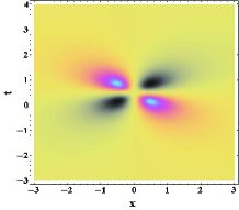
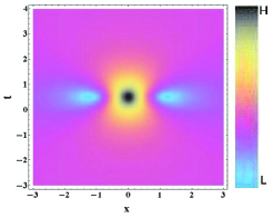
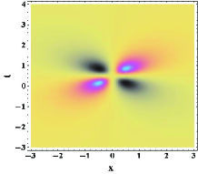
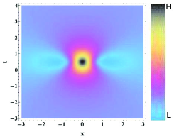
Figure 1: (color online) The evolution plot of one RW in coupled system, (a) for one RW in $\psi_{1}$ component, (b) for one RW in $\psi_{2}$ component, (c) for one RW in $\psi_{3}$ component. (d) for the whole density of the three components. It is seen that the density distribution shapes of RW in $\psi_{1}$ and $\psi_{3}$ are different from the eyes shape. The coefficients are $A_{1}=0,A_{2}=1,A_{3}=0$, and $A_{4}=0$. The ”L” and ”S” in color bar denote large and small values of density respectively. This holds for all figures.

One vector rouge wave— When $A_{3}=0,A_{4}=0$, only one vector RW can be observed in all components, as shown in Fig. 1. Interestingly, we find that there is a novel shape for vector RW solution. The density distribution shapes of the localized waves in $\psi_{1}$ and $\psi_{3}$ are quite different from the well-known eye-shaped one. There are two humps and two valleys around a center, and the center’s value is almost equal to that of the background, as shown in Fig. 1(a) and (c). This structure can be called as four-petaled structure in temporal-spatial distribution. Moreover, the humps or valleys in $\psi_{1}$ correspond to the valleys or humps in $\psi_{3}$. However, the density distribution in $\psi_{2}$ is similar to the eye shaped RW in single-component system, as shown in Fig. 1(b). Therefore, the whole density is still the well known eyes shape, as shown in Fig. 1(d). The novel shape should come from the cross phase modulation effects, since the shape can not be observed in scalar RW. For two-component coupled systems, it has been found numerically that there are dark RWs in one component of the coupled system in Bludov . The dark RW has been given exactly in our previous paper in zhao2 . Based on these results, we expect that there should be some novel structures in more than three modes coupled systems.

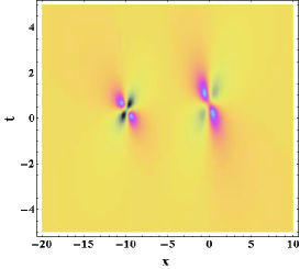
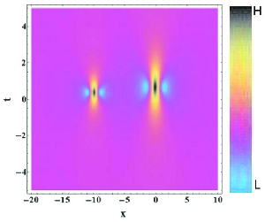
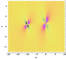
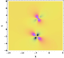
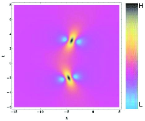
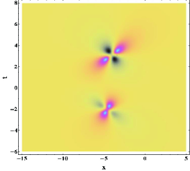
Figure 2: (color online) The evolution plot of two vector RWs in coupled system, (a) for the RWs in $\psi_{1}$ component, (b) for the RWs in $\psi_{2}$ component. (c) for the RWs in $\psi_{3}$ component. The coefficients are $A_{1}=0,A_{2}=40,A_{3}=8$, and $A_{4}=0$. (d), (e) and (f) show the evolution of RWs in $\psi_{1}$, $\psi_{2}$, and $\psi_{3}$ respectively. The coefficients are $A_{1}=150,A_{2}=40,A_{3}=8$, and $A_{4}=0$.

Two vector rouge waves— When $A_{4}=0$, there are two vector RWs appearing in the temporal-spatial distribution, shown in Fig. 2. When $A_{1}\leq 0$, there are two vector RWs emerging at a certain propagation distance, as shown in Fig. 2(a)-(c). It is seen that the structures of the two RWs in every mode are similar, and only the sizes are different. The four-petaled structure RWs emerge in $\psi_{1,3}$ and the eye-shaped ones emerge in $\psi_{2}$ component. When $A_{1}>>0$, the two distinct RWs emerge at different propagation distances, shown in Fig. 2(d)-(f). There is a rotation on $x-t$ distribution plane for the two RWs. Varying the parameter $A_{1,3}$, one can observe the interactions between the two RWs.

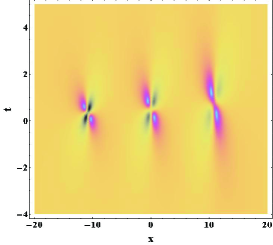
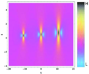
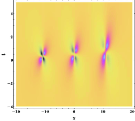
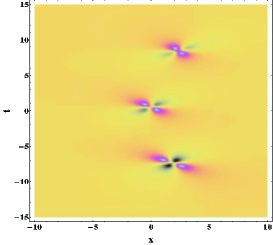
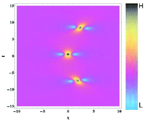
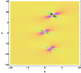
Figure 3: (color online) The evolution plot of three vector RWs in coupled system, (a) for the RWs in $\psi_{1}$ component, (b) for the RWs in $\psi_{2}$ component. (c) for the RWs in $\psi_{3}$ component. The coefficients are $A_{1}=0,A_{2}=20,A_{3}=0$, and $A_{4}=-1$. (d), (e) and (f) show the evolution of RWs in $\psi_{1}$, $\psi_{2}$, and $\psi_{3}$ respectively. The coefficients are $A_{1}=0,A_{2}=20,A_{3}=0$, and $A_{4}=1$.

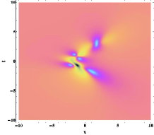
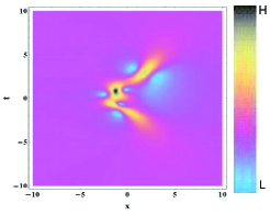
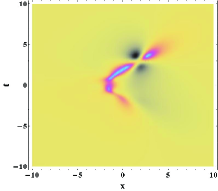
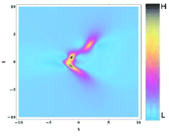
Figure 4: (color online) The interaction plot of three RWs in the coupled system, (a) for the RWs in $\psi_{1}$ component, (b) for the RWs in $\psi_{2}$ component, (c) for the RWs in $\psi_{3}$ component. (d) for the whole density of the three components. The coefficients are $A_{1}=0,A_{2}=1,A_{3}=1$, and $A_{4}=1$.

Three vector rouge waves— When $A_{4}\neq 0$, there are three vector RWs appearing in the temporal-spatial distribution, as shown in Fig. 3. When $A_{4}A_{2}<0$ and $|A_{2}|>>|A_{4}|$, there are three vector RWs emerging very clearly at a certain propagation distance, as shown in Fig. 3(a)-(c). The structures of them in each component are similar with different sizes. The valleys in $\psi_{1}$ still correspond to the humps in $\psi_{3}$ component. There are three eye- shaped RWs in $\psi_{2}$. When $A_{4}A_{2}>0$ and $|A_{2}|>>|A_{4}|$, the three RW emerge clearly at different propagation distances, as shown in Fig. 3(d)-(f). The RW seems to have changing velocity on retarded time. Varying the parameters, we can investigate the interaction between these vector RWs conveniently. For example, making $A_{2}$ approach $A_{4}$, we can observe the interaction of the three RWs, such as Fig. 4. It shows that RW’s shape can be changed greatly through interacting with others. Two RWs almost fuse to one valley in $\psi_{3}$ component with the condition, as shown in Fig. 4(c).

It should be noted that the distribution shapes of the two and three RWs in the whole temporal-spatial distribution are very distinct from the high-order RW in one-component system presented in Ling ; Akhmediev ; Yang . In the one-component systems, it is not possible to observe just two RWs appearing in the whole temporal-spatial distribution even for high-order RWs. Three RWs can emerge on temporal-spatial distribution for second-order scalar RW, but their distribution shapes are different from the three RWs obtained here. Therefore, we call the generalized vector RW solution as multi-vector RW.

III Possibilities to observe these vector nonlinear waves

Considering the experiments on RW in nonlinear fibers D.R. Solli , which have shown that the simple scalar NLS could describe nonlinear waves in nonlinear fibers well, we expect that these different vector RWs could be observed in three-mode nonlinear fibers. One could introduce three-mode optical signals into a nonlinear fiber operating in the anomalous group velocity dispersion regime, marked by $\psi_{j}$ ($j=1,2,3$). Firstly, we assume the nonlinear coefficients for the three modes are equal. The dispersion and nonlinear coefficients are $1$ and $2$ in normalized units respectively. Then, the backgrounds can be given by Eq.(5) and (6). Explicitly, the amplitude of $\psi_{1}$ is set to be $s_{1}$, the amplitude of $\psi_{2}$ is $s_{2}=\frac{\sqrt{2}}{2}s_{1}$, and the amplitude of $\psi_{3}$ is $s_{3}=s_{1}$. The wave vector of $\psi_{2}$ marked by $k_{2}$ is set to be zero, and the wave vectors of $\psi_{1}$ and $\psi_{3}$ are $k_{1}=-k_{3}$, and $k_{3}=\frac{\sqrt{2}}{2}s_{1}$. Then the initial optical signals are given by the presented vector RW solution Eq.(7)-(9). For nonlinear fibers, the coordinates $x$ and $t$ should be changed to be $t$ and $z$, which are retarded time and propagation distance respectively. Under the corresponding conditions, one, two, or three vector RWs could be observed in the nonlinear fiber.

On the other hand, it is well known that there are spatial optical solitons in planar waveguide. The similar conditions can be derived directly through coordinates transformation for the coupled NLS in a planar waveguide Cambournac . The RWs in multi-mode planar waveguide could be observed too. Additionally, considering the studies on multi-components Bose-Einstein condensates Das ; Becker ; Engels , we expect that the vector RWs could also be observed with the condition.

IV Discussion and Conclusion

In summary, we find some novel structures for vector RWs in a three-component coupled system. The novel shape lies in that there are two humps and two valleys around one center in the temporal-spatial distribution. The obtained multi-vector RW solution can be used to describe one, two, and even three vector RWs in the coupled system, whose density distribution shapes are different from high-order scalar RW. The corresponding conditions for their emergence are presented explicitly. Under these conditions, the ideal initial signals for them can be given from the generalized rational solution, which could be helpful for experimental observation. Based on these results, we expect that abundant novel structures could exist in more-than-three-component coupled systems.

The coupled system can be used to describe three-component BEC, multi-mode optical transmission, and so on. Therefore, we believe that these nonlinear waves can be observed experimentally. As an example, the possible way to observe vector RWs in three-mode nonlinear fiber is discussed here. Recently, the high-order modulation instability with RWs has been observed in nonlinear fiber optics in Erkintalo . There are many possibilities to observe similar phenomena in coupled nonlinear fiber system.

Appendix A: The analytic expressions for $H_{j}(x,t)$ and $G_{j}(x,t)$

$$H_{1} = -(1+i)\left[6iA_{1}+(6-6i)A_{3}-6i\sqrt{2}A_{4}+(6+12i)A_{3}t+6\sqrt{2}A_{4}t-6iA_{3}t^{2}-(6-6i)\sqrt{2}A_{4}t^{2}+2\sqrt{2}A_{4}t^{3}\right.$$

$$\left.+A_{2}(6\sqrt{2}-6\sqrt{2}t+6ix)+6\sqrt{2}A_{3}x+(6-6i)A_{4}x-6\sqrt{2}A_{3}tx+(6+12i)A_{4}tx-6iA_{4}t^{2}x+3iA_{3}x^{2}\right.$$

$$\left.+3\sqrt{2}A_{4}x^{2}-3\sqrt{2}A_{4}tx^{2}+iA_{4}x^{3}\right]\left[6\sqrt{2}A_{1}+(6+12i)\sqrt{2}A_{3}t-(6+6i)A_{4}t-6\sqrt{2}A_{3}t^{2}+(18-6i)A_{4}t^{2}\right.$$

$$\left.+4iA_{4}t^{3}-(6-6i)A_{3}x-12iA_{3}tx+(6+12i)\sqrt{2}A_{4}tx-6\sqrt{2}A_{4}t^{2}x+3\sqrt{2}A_{3}x^{2}-(3-3i)A_{4}x^{2}-6iA_{4}tx^{2}\right.$$

$$\left.+\sqrt{2}A_{4}x^{3}+6A_{2}(-1+i-2it+\sqrt{2}x)\right],$$

$$G_{1} = \sqrt{2}\left[36A_{1}^{2}+36A_{3}^{2}+54\sqrt{2}A_{3}A_{4}+54A_{4}^{2}+108A_{3}^{2}t^{2}-36\sqrt{2}A_{3}A_{4}t^{2}-72A_{3}^{2}t^{3}+48\sqrt{2}A_{3}A_{4}t^{3}-24A_{4}^{2}t^{3}\right.$$

$$\left.+36A_{3}^{2}t^{4}-48\sqrt{2}A_{3}A_{4}t^{4}+108A_{4}^{2}t^{4}-24A_{4}^{2}t^{5}+8A_{4}^{2}t^{6}+36\sqrt{2}A_{3}^{2}x+108A_{3}A_{4}x+54\sqrt{2}A_{4}^{2}x-72\sqrt{2}A_{3}^{2}t^{2}x\right.$$

$$\left.+144A_{3}A_{4}t^{2}x-36\sqrt{2}A_{4}^{2}t^{2}x-48A_{3}A_{4}t^{3}x+48\sqrt{2}A_{4}^{2}t^{3}x+24A_{3}A_{4}t^{4}x-48\sqrt{2}A_{4}^{2}t^{4}x+36A_{3}^{2}x^{2}+54\sqrt{2}A_{3}A_{4}x^{2}\right.$$

$$\left.+54A_{4}^{2}x^{2}-36A_{3}^{2}tx^{2}+36A_{3}^{2}t^{2}x^{2}-72\sqrt{2}A_{3}A_{4}t^{2}x^{2}+72A_{4}^{2}t^{2}x^{2}-24A_{4}^{2}t^{3}x^{2}+12A_{4}^{2}t^{4}x^{2}+36A_{3}A_{4}x^{3}\right.$$

$$\left.+18\sqrt{2}A_{4}^{2}x^{3}-24A_{3}A_{4}tx^{3}+24A_{3}A_{4}t^{2}x^{3}-24\sqrt{2}A_{4}^{2}t^{2}x^{3}+9A_{3}^{2}x^{4}+9A_{4}^{2}x^{4}-6A_{4}^{2}tx^{4}+6A_{4}^{2}t^{2}x^{4}+6A_{3}A_{4}x^{5}\right.$$

$$\left.-12A_{2}(-3A_{4}+6A_{4}t^{2}-8A_{4}t^{3}+4A_{4}t^{4}-3A_{4}\sqrt{2}x-3A_{4}x^{2}-A_{4}x^{4}+6A_{3}\sqrt{2}t^{2}-6A_{3}t^{2}x+6A_{3}tx-3\sqrt{2}A_{3})\right.$$

$$\left.+12A_{1}(6A_{2}x+6A_{3}t-6A_{3}t^{2}+3A_{3}x^{2}+6\sqrt{2}A_{4}t^{2}-6A_{4}t^{2}x+6A_{4}tx+A_{4}x^{3})\right.$$

$$\left.+72A_{2}A_{3}x+36A_{2}A_{3}x^{3}+A_{4}^{2}x^{6}+36A_{2}^{2}(1-2t+2t^{2}+x^{2})\right].$$

$$H_{2} = 72\sqrt{2}A_{1}^{2}+72i\sqrt{2}A_{2}^{2}+(72-72i)\sqrt{2}A_{1}A_{3}+144iA_{2}A_{3}+(144-144i)A_{1}A_{4}+144i\sqrt{2}A_{2}A_{4}-(144+144i)\sqrt{2}A_{2}^{2}t$$

$$+(144+144i)\sqrt{2}A_{1}A_{3}t+(216+72i)\sqrt{2}A_{3}^{2}t-(288+144i)\sqrt{2}A_{2}A_{4}t+(288+144i)A_{3}A_{4}t-144\sqrt{2}A_{4}^{2}t+144\sqrt{2}A_{2}^{2}t^{2}$$

$$-144\sqrt{2}A_{1}A_{3}t^{2}-288A_{2}A_{3}t^{2}+216i\sqrt{2}A_{3}^{2}t^{2}+288A_{1}A_{4}t^{2}+(144-288i)\sqrt{2}A_{2}A_{4}t^{2}-144A_{3}A_{4}t^{2}$$

$$+(144-360i)\sqrt{2}A_{4}^{2}t^{2}-(144+144i)\sqrt{2}A_{3}^{2}t^{3}+(192+192i)\sqrt{2}A_{2}A_{4}t^{3}+(192+192i)A_{3}A_{4}t^{3}+(192+48i)\sqrt{2}A_{4}^{2}t^{3}$$

$$+72\sqrt{2}A_{3}^{2}t^{4}-96\sqrt{2}A_{2}A_{4}t^{4}-192A_{3}A_{4}t^{4}+(96+120i)\sqrt{2}A_{4}^{2}t^{4}-(48+48i)\sqrt{2}A_{4}^{2}t^{5}+16\sqrt{2}A_{4}^{2}t^{6}+144\sqrt{2}A_{1}A_{2}x$$

$$+(72+72i)\sqrt{2}A_{2}A_{3}x+144iA_{3}^{2}x+(72-72i)\sqrt{2}A_{1}A_{4}x+144A_{2}A_{4}x+144i\sqrt{2}A_{3}A_{4}x-(144+144i)\sqrt{2}A_{2}A_{3}tx$$

$$+(144+144i)\sqrt{2}A_{1}A_{4}tx+144\sqrt{2}A_{3}A_{4}tx+(288+144i)A_{4}^{2}tx+144\sqrt{2}A_{2}A_{3}t^{2}x-288A_{3}^{2}t^{2}x$$

$$-144\sqrt{2}A_{1}A_{4}t^{2}x+(144+144i)\sqrt{2}A_{3}A_{4}t^{2}x-144A_{4}^{2}t^{2}x-(96+96i)\sqrt{2}A_{3}A_{4}t^{3}x+(192+192i)A_{4}^{2}t^{3}x$$

$$+48\sqrt{2}A_{3}A_{4}t^{4}x-192A_{4}^{2}t^{4}x+72\sqrt{2}A_{2}^{2}x^{2}+72\sqrt{2}A_{1}A_{3}x^{2}+(36+36i)\sqrt{2}A_{3}^{2}x^{2}+72\sqrt{2}A_{2}A_{4}x^{2}$$

$$+(72+144i)A_{3}A_{4}x^{2}+72i\sqrt{2}A_{4}^{2}x^{2}-(72+72i)\sqrt{2}A_{3}^{2}tx^{2}+72\sqrt{2}A_{4}^{2}tx^{2}+72\sqrt{2}A_{3}^{2}t^{2}x^{2}+12\sqrt{2}A_{4}^{2}t^{2}x^{4}$$

$$-288A_{3}A_{4}t^{2}x^{2}+(72+72i)\sqrt{2}A_{4}^{2}t^{2}x^{2}-(48+48i)\sqrt{2}A_{4}^{2}t^{3}x^{2}+24\sqrt{2}A_{4}^{2}t^{4}x^{2}+72\sqrt{2}A_{2}A_{3}x^{3}+2\sqrt{2}A_{4}^{2}x^{6}$$

$$+24\sqrt{2}A_{1}A_{4}x^{3}+(48+24i)\sqrt{2}A_{3}A_{4}x^{3}+(24+48i)A_{4}^{2}x^{3}-(48+48i)\sqrt{2}A_{3}A_{4}tx^{3}+48\sqrt{2}A_{3}A_{4}t^{2}x^{3}$$

$$-96A_{4}^{2}t^{2}x^{3}+18\sqrt{2}A_{3}^{2}x^{4}+24\sqrt{2}A_{2}A_{4}x^{4}+(12+6i)\sqrt{2}A_{4}^{2}x^{4}-(12+12i)\sqrt{2}A_{4}^{2}tx^{4}+12\sqrt{2}A_{3}A_{4}x^{5},$$

$$G_{2} = 36\sqrt{2}A_{1}^{2}+36\sqrt{2}A_{2}^{2}+72A_{2}A_{3}+36\sqrt{2}A_{3}^{2}+36\sqrt{2}A_{2}A_{4}+108A_{3}A_{4}+54\sqrt{2}A_{4}^{2}-72\sqrt{2}A_{2}^{2}t$$

$$+72\sqrt{2}A_{1}A_{3}t+72\sqrt{2}A_{2}^{2}t^{2}-72\sqrt{2}A_{1}A_{3}t^{2}-144A_{2}A_{3}t^{2}+108\sqrt{2}A_{3}^{2}t^{2}+12\sqrt{2}A_{2}A_{4}x^{4}$$

$$+144A_{1}A_{4}t^{2}-72\sqrt{2}A_{2}A_{4}t^{2}-72A_{3}A_{4}t^{2}-72\sqrt{2}A_{3}^{2}t^{3}+96\sqrt{2}A_{2}A_{4}t^{3}+96A_{3}A_{4}t^{3}-24\sqrt{2}A_{4}^{2}t^{3}$$

$$+36\sqrt{2}A_{3}^{2}t^{4}-48\sqrt{2}A_{2}A_{4}t^{4}-96A_{3}A_{4}t^{4}+108\sqrt{2}A_{4}^{2}t^{4}-24\sqrt{2}A_{4}^{2}t^{5}+8\sqrt{2}A_{4}^{2}t^{6}+72\sqrt{2}A_{1}A_{2}x$$

$$+72\sqrt{2}A_{2}A_{3}x+72A_{3}^{2}x+72A_{2}A_{4}x+108\sqrt{2}A_{3}A_{4}x+108A_{4}^{2}x-72\sqrt{2}A_{2}A_{3}tx+72\sqrt{2}A_{1}A_{4}tx$$

$$+72\sqrt{2}A_{2}A_{3}t^{2}x-144A_{3}^{2}t^{2}x-72\sqrt{2}A_{1}A_{4}t^{2}x+144\sqrt{2}A_{3}A_{4}t^{2}x-72A_{4}^{2}t^{2}x-48\sqrt{2}A_{3}A_{4}t^{3}x$$

$$+96A_{4}^{2}t^{3}x+24\sqrt{2}A_{3}A_{4}t^{4}x-96A_{4}^{2}t^{4}x+36\sqrt{2}A_{2}^{2}x^{2}+36\sqrt{2}A_{1}A_{3}x^{2}+36\sqrt{2}A_{3}^{2}x^{2}+\sqrt{2}A_{4}^{2}x^{6}$$

$$+36\sqrt{2}A_{2}A_{4}x^{2}+108A_{3}A_{4}x^{2}+54\sqrt{2}A_{4}^{2}x^{2}-36\sqrt{2}A_{3}^{2}tx^{2}+36\sqrt{2}A_{3}^{2}t^{2}x^{2}-144A_{3}A_{4}t^{2}x^{2}$$

$$+72\sqrt{2}A_{4}^{2}t^{2}x^{2}-24\sqrt{2}A_{4}^{2}t^{3}x^{2}+12\sqrt{2}A_{4}^{2}t^{4}x^{2}+36\sqrt{2}A_{2}A_{3}x^{3}+12\sqrt{2}A_{1}A_{4}x^{3}$$

$$+36\sqrt{2}A_{3}A_{4}x^{3}+36A_{4}^{2}x^{3}-24\sqrt{2}A_{3}A_{4}tx^{3}+24\sqrt{2}A_{3}A_{4}t^{2}x^{3}-48A_{4}^{2}t^{2}x^{3}+9\sqrt{2}A_{3}^{2}x^{4}$$

$$+9\sqrt{2}A_{4}^{2}x^{4}-6\sqrt{2}A_{4}^{2}tx^{4}+6\sqrt{2}A_{4}^{2}t^{2}x^{4}+6\sqrt{2}A_{3}A_{4}x^{5}.$$

$$H_{3} = (1+i)\left[6A_{1}-6iA_{3}t-6A_{3}t^{2}+6\sqrt{2}A_{4}t^{2}-2i\sqrt{2}A_{4}t^{3}+6i\sqrt{2}A_{3}tx-6iA_{4}tx-6A_{4}t^{2}x+3A_{3}x^{2}+3i\sqrt{2}A_{4}tx^{2}\right.$$

$$\left.+A_{4}x^{3}+6A_{2}\left(i\sqrt{2}t+x\right)\right]\left[6\sqrt{2}A_{1}+(6+12i)\sqrt{2}A_{3}t-(6+6i)A_{4}t-6\sqrt{2}A_{3}t^{2}+(18-6i)A_{4}t^{2}+4iA_{4}t^{3}\right.$$

$$\left.-(6-6i)A_{3}x-12iA_{3}tx+(6+12i)\sqrt{2}A_{4}tx-6\sqrt{2}A_{4}t^{2}x+3\sqrt{2}A_{3}x^{2}-(3-3i)A_{4}x^{2}\right.$$

$$\left.-6iA_{4}tx^{2}+\sqrt{2}A_{4}x^{3}+6A_{2}\left((-1+i)-2it+\sqrt{2}x\right)\right],$$

$$G_{3} = \sqrt{2}\left[36A_{1}^{2}+36A_{3}^{2}+54\sqrt{2}A_{3}A_{4}+54A_{4}^{2}+108A_{3}^{2}t^{2}-36\sqrt{2}A_{3}A_{4}t^{2}-72A_{3}^{2}t^{3}\right.$$

$$\left.+48\sqrt{2}A_{3}A_{4}t^{3}-24A_{4}^{2}t^{3}+36A_{3}^{2}t^{4}-48\sqrt{2}A_{3}A_{4}t^{4}+108A_{4}^{2}t^{4}-24A_{4}^{2}t^{5}+8A_{4}^{2}t^{6}+36\sqrt{2}A_{3}^{2}x\right.$$

$$\left.+108A_{3}A_{4}x+54\sqrt{2}A_{4}^{2}x-72\sqrt{2}A_{3}^{2}t^{2}x+144A_{3}A_{4}t^{2}x-36\sqrt{2}A_{4}^{2}t^{2}x-48A_{3}A_{4}t^{3}x\right.$$

$$\left.+48\sqrt{2}A_{4}^{2}t^{3}x+24A_{3}A_{4}t^{4}x-48\sqrt{2}A_{4}^{2}t^{4}x+36A_{3}^{2}x^{2}+54\sqrt{2}A_{3}A_{4}x^{2}+54A_{4}^{2}x^{2}-36A_{3}^{2}tx^{2}\right.$$

$$\left.+36A_{3}^{2}t^{2}x^{2}-72\sqrt{2}A_{3}A_{4}t^{2}x^{2}+72A_{4}^{2}t^{2}x^{2}-24A_{4}^{2}t^{3}x^{2}+12A_{4}^{2}t^{4}x^{2}+36A_{3}A_{4}x^{3}\right.$$

$$\left.-12A_{2}\left(A_{4}(-3+6t^{2}-8t^{3}+4t^{4}-3\sqrt{2}x-3x^{2}-x^{4})+A_{3}(6t^{2}\sqrt{2}-6t^{2}x+6tx-3\sqrt{2}-6x-3x^{3})\right)\right.$$

$$\left.+12A_{1}\left(6A_{2}x+A_{3}(6t-6t^{2}+3x^{2})+A_{4}(6t^{2}\sqrt{2}-6t^{2}x+6tx+x^{3})\right)\right.$$

$$\left.+18\sqrt{2}A_{4}^{2}x^{3}-24A_{3}A_{4}tx^{3}+24A_{3}A_{4}t^{2}x^{3}-24\sqrt{2}A_{4}^{2}t^{2}x^{3}+9A_{3}^{2}x^{4}+9A_{4}^{2}x^{4}-6A_{4}^{2}tx^{4}\right.$$

$$\left.+6A_{4}^{2}t^{2}x^{4}+6A_{3}A_{4}x^{5}+A_{4}^{2}x^{6}+36A_{2}^{2}(1-2t+2t^{2}+x^{2})\right].$$

References

• (1) N. Akhmediev, J.M. Soto-Crespo, A. Ankiewicz, Phys. Lett. A 373, 2137-2145 (2009).
• (2) C. Kharif and E. Pelinovsky, Eur. J. Mech. B/Fluids 22, 603 (2003).
• (3) D.R. Solli, C. Ropers, P. Koonath, B. Jalali, Nature 450, 06402 (2007); B. Kibler, J. Fatome, C. Finot, G. Millot, et al., Nature Phys. 6, 790 (2010).
• (4) A. Chabchoub, N.P. Hoffmann, and N. Akhmediev, Phys. Rev. Lett. 106, 204502 (2011).
• (5) A. Ankiewicz, J. M. Soto-Crespo, and Nail Akhmediev, Phys. Rev. E 81, 046602 (2010).
• (6) N. Akhmediev, A. Ankiewicz, M. Taki, Phys. Lett. A 373, 675-678 (2009).
• (7) V. V. Voronovich, V. I. Shrira, and G. Thomas, J. Fluid Mech. 604, 263 (2008).
• (8) N. Akhmediev, A. Ankiewicz, and J. M. Soto-Crespo, Phys. Rev. E 80, 026601 (2009).
• (9) F. Baronio, A. Degasperis, M. Conforti, and S. Wabnitz, Phys. Rev. Lett. 109, 044102 (2012).
• (10) B.L. Guo, L.M. Ling, Chin. Phys. Lett. 28, 110202 (2011).
• (11) Y.V. Bludov, V.V. Konotop, and N. Akhmediev, Eur. Phys. J. Special Topics 185, 169 (2010).
• (12) L.C. Zhao, J. Liu, Joun. Opt. Soc. Am. B 29, 3119-3127 (2012).
• (13) M. Vijayajayanthi, T. Kanna, and M. Lakshmanan, Phys. Rev. A 77, 013820 (2008); M. Vijayajayanthi, T. Kanna and M. Lakshmanan, Europ. Phys. Journ. - Special Topics 173, 57-80 (2009).
• (14) L.C. Zhao, S.L. He, Phys. Lett. A 375, 3017-3020 (2011).
• (15) B.L. Guo, L.M. Ling, Q. P. Liu , Phys. Rev. E 85, 026607 (2012).
• (16) Y. Ohta and J.K. Yang, Proc. R. Soc. A 468, 1716-1740 (2012).
• (17) C. Cambournac, T. Sylvestre, H. Maillotte, B. Vanderlinden, P. Kockaert, Ph. Emplit, and M. Haelterman, Phys. Rev. Lett. 89, 083901 (2002).
• (18) P. Das, T.S. Raju, U. Roy, and Prasanta K. Panigrahi, Phys. Rev. A 79, 015601 (2009).
• (19) C. Becker, S. Stellmer, P.S. Panahi, S. Dorscher, M. Baumert, Eva-Maria Richter, Jochen Kronjager, Kai Bongs,Klaus Sengstock, Nature phys. 4, 496-501 (2008).
• (20) C. Hamner, J. J. Chang, and P. Engels, Phys. Rev. Lett. 106, 065302 (2011); M. A. Hoefer, J. J. Chang, C. Hamner, and P. Engels, Phys. Rev. A 84, 041605(R) (2011).
• (21) M. Erkintalo, K. Hammani, B. Kibler,C. Finot, N. Akhmediev, J. M. Dudley, and G. Genty, Phys. Rev. Lett. 107, 253901 (2011).