The Local-time variations of Lunar Prospector epithermal-neutron data

Abstract

We assess local-time variations of epithermal-neutron count rates measured by the Lunar Prospector Neutron Spectrometer. We investigate the nature of these variations and find no evidence to support the idea that such variations are caused by diurnal variations of hydrogen concentration across the lunar surface. Rather we find an anticorrelation between instrumental temperature and epithermal-neutron count rate. We have also found that the measured counts are dependent on the temperatures of the top decimeters of the lunar subsurface as constrained by the Lunar Reconnaissance Orbiter Diviner Lunar Radiometer Experiment temperature measurements. Finally, we have made the first measurement of the effective leakage depth for epithermal-neutrons of $\sim$20 cm.

1 Introduction

The mapping of hydrogen on the near surface of the Moon has been one of the focal points of the exploration of the Moon. Neutron spectroscopy has been central to this endeavor and allows one to probe the top few decimeters [e.g. Feldman et al., 1998, Lawrence et al., 2006]. Neutron spectrometers detect leakage neutrons resulting from the interaction of galactic cosmic rays (GCR) and the chemical elements present in the top layers of the planetary subsurface. These neutrons lose energy by interacting with the surrounding lunar material, and different elastic and inelastic scattering cross-sections produce different amounts of moderation and capture. Since the Moon has no atmosphere, cosmic rays reach the surface without being absorbed and neutrons can leak from the near subsurface without being scattered further or absorbed. In addition, the Moon has a characteristic composition pattern (dichotomy between Fe and Ti-rich maria and Al-rich highlands), to which neutron measurements are highly sensitive. Finally, from returned samples, the lunar regolith is recognized to be hydrogen poor at equatorial latitudes [$<$100 ppm, Heiken et al., 1991]. This a priori information has played a major role in the interpretation and understanding of the orbital neutron data.

According to their kinetic energy, $E_{\mbox{\scriptsize{kin}}}$, neutrons are typically divided into three different energy bands: fast, epithermal and thermal. These correspond to $E_{\mbox{\scriptsize{kin}}}>0.5\mbox{~{}MeV}$, $0.4\mbox{~{}eV}$ $<~{}E_{\mbox{\scriptsize{kin}}}~{}<~{}0.5\mbox{~{}MeV}$ and $E_{\mbox{\scriptsize{kin}}}\leq~{}0.4\mbox{~{}eV}$ respectively. Briefly, thermal neutrons are particularly sensitive to Fe, Ti, Gd and Sm in the absence of H [Elphic et al., 1998, 2000]. Epithermal-neutrons are strongly moderated by H [Feldman et al., 1993] and therefore provide a robust measure of H concentrations and their spatial variations. Multiple studies have reported the presence and concentrations of H enhancements at the lunar poles [Feldman et al., 1998, Eke et al., 2009, Teodoro et al., 2010, 2014] as well as H concentrations within non-polar regions [Lawrence et al., 2015].

In this article we study the daily variations of epithermal-neutron count rates from the Lunar Prospector neutron spectrometer (LPNS) to inquire if such potential variations are sensitive to daily variations in H concentrations. This study is prompted, in part, by a report of time-variable concentrations of surficial (top tens of micrometers) H₂O/OH that have been observed with spectral reflectance data [Sunshine et al., 2009]. If such time variable H concentrations extend to macroscopic depths of multiple mm to cm [Lawrence et al., 2011], then such variations could in principle be observed with orbital neutron data. Preliminary analysis of data from the Lunar Exploration Neutron Detector (LEND) on the NASA Lunar Reconnaissance Orbiter (LRO) mission has shown a diurnal count rate variation, which has been interpreted as daily variations in H concentrations [Livengood et al., 2014]. Such findings, if confirmed, could lead to important consequences to our understanding of the hydrogen distribution at the lunar surface. Here, we will show that LPNS epithermal-neutron count rates also show variations with solar local time, but that these variations are anti correlated with variations in instrumental temperature. Furthermore, the LPNS daily variations show a dependence on the temperatures at the top few decimeters of the lunar subsurface as predicted by the numerical work of Little et al. [2003] and Lawrence et al. [2006]. These findings suggest that rather than reflecting diurnal changes in the hydrogen content of the lunar regolith, the temporal fluctuations in the count rates are due to small residual systematic effects in the data reduction.

In Section 2 we present the datasets used throughout the article while in Section 3 we perform the analysis of the epithermal dataset. We finish the article in Section 4 with our conclusions and discussion.

2 Datasets

In this section we will briefly detail the main characteristics of the epithermal-neutron dataset gathered by the LPNS, which is in the public domain at the Planetary Data System (PDS) (http://pds-geosciences.wustl.edu/missions/lunarp/). We will also use temperature measurements of the lunar surface collected by the Diviner Lunar Radiometer on Lunar Reconnaissance Orbiter. These measurements are also available at PDS (http://pds-geosciences.wustl.edu/missions/lro/diviner.htm).

2.1 LPNS Counting data

The Lunar Prospector Neutron Spectrometer, designed and built at the Los Alamos National Laboratory, consists of two gas proportional counters containing helium-3. The neutrons that are captured by helium-3 nuclei within the detectors produce a unique energy signature that is then detected and counted. The two sensors have different covers: one is covered in cadmium, the other in tin. The cadmium cover screens out thermal neutrons while the tin counterpart does not. Differences in the counts between the two tubes thus quantify the detected number of thermal neutrons. The neutron spectrometer was located at the end of a 2.5 m boom, thus reducing the background from the main body of the spacecraft. For further details regarding the neutron spectrometer see Feldman et al. [2004].

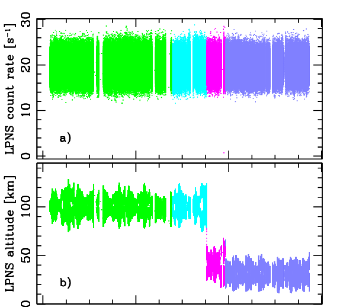
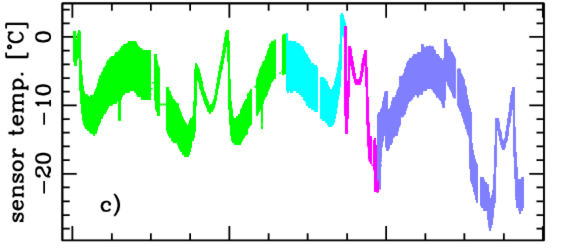
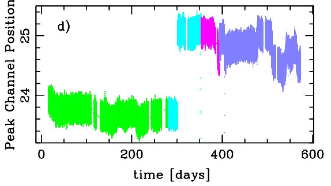
Figure 1: a) Measured 8s counting rates and b) spacecraft altitude versus time. We are only considering data in which $|\mbox{latitude}|<55^{{}^{\circ}}$. The colour scheme denotes different phases of the Lunar Prospector mission: : High 1 (green), High 2 (cyan), magenta (Low 1), violet (Low 2). The origin of the global time was set at 1st of January 1998. The individual counting rates were normalized to an altitude of 30 km [Maurice et al., 2004]. c) Neutron sensor temperature. d) Peak-channel position of the 764 keV neutron-capture peak in the LPNS pulse height spectra (see Figure 5). The large jump in peak channel-position around time $\sim$300 days coincides with an increase in the sensor’s high voltage.

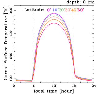
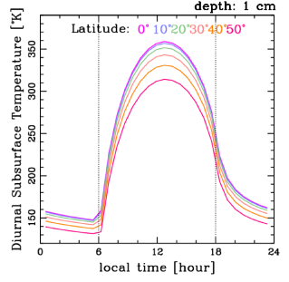
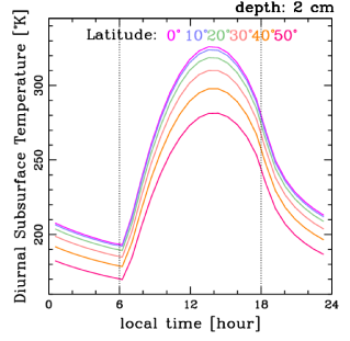
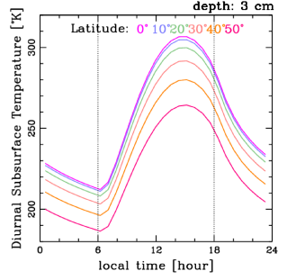
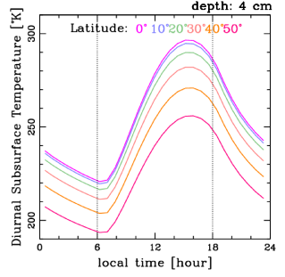
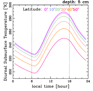
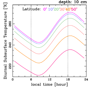
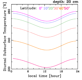
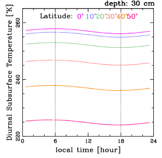
Figure 2: Upper left Diviner Temperature measurements at different latitudes function of the lunar local time. From the left to the right, and from the top to the bottom we show subsurface temperatures drawn from Diviner thermal models at 1, 2, 3, 4, 5, 10, 20 and 30 cm deep, respectively. These temperatures have been constrained by the Diviner observations using the methodology detailed in Siegler et al. [2011].

The epithermal-neutron counting rate and spacecraft altitude time series are shown in Figure 1, along with other parameters (neutron sensor temperature and pulse height peak-channel position) used in this study. All data shown in Figure 1 are coloured based on the different mission phases described in Table 2 of Maurice et al. [2004]. Green shows data from the High 1 phase (average altitude $\sim$100 km), cyan shows data from the High 2 phase (average altitude $\sim$100 km, flipped spacecraft spin axis), magenta shows data from the Low 1 phase (average altitude $\sim$40 km), and violet shows data from the Low 2 phase (average altitude $\sim$30 km). The origin of time was set at 1st of January 1998

Hereafter we will use data within the latitude range $[-55^{\circ},$ $55^{\circ}]$, coming either from the High 1 (hereafter High Altitude) or Low 2 (hereafter, Low-altitude) phases, respectively. A third dataset with all the measurements within the same latitude range will be termed Overall. The number of 8s measurements within Overall, High altitude and Low-altitude datasets are 2,851,632, 1,324,569 and 939,668, respectively. With this choice of latitudes we are considering those parts of the lunar surface whose epithermal signal is not dominated by the hydrogen enhancements in the top few decimeters of regolith. The individual count rates were normalized to altitude 30 km [Maurice et al., 2004].

2.2 Lunar Prospector Instrumental Temperature and Energy spectrum information

The LPNS included a temperature sensor. Its time-series variation is presented in panel c) of Figure 1. As with the count rate data we will use data within $|\mbox{latitude}|<55^{{}^{\circ}}$.

The LPNS returned pulse height spectra of the ³He neutron captures, and a key feature is the 764 keV full-energy capture peak (see Figure 5). Panel d) of Figure 1 shows the Cd ³He sensor peak-channel position versus time. The large jump in peak-channel position around time $\sim$300 days coincides with an increase in the detector’s high voltage.

2.3 Diviner/LRO temperature diurnal variation data

The Diviner Lunar Radar Experiment on board LRO is an imaging multi-channel solar reflectance and infrared radiometer. This instrument maps the temperature of the lunar surface at $<$ 500 meter horizontal scales. Diviner data sets are produced by the Diviner Science Team at the University of California, Los Angeles.

Here we use temperature information as function of the lunar local time at different depths of the lunar subsurface. We will employ the Diviner measurements and model predictions constrained by such measurements [see Siegler et al., 2011, for details]. Upper left panel in Figure 2 shows the Diviner measurements and the remaining eight panels show the model’s predictions at depths of 1, 2, 3, 4, 5, 10, 20 and 30 cm.

As expected, subsurface temperatures have a strong dependence on the local time, depth and latitude. At the surface, temperature peaks at the local midday. At deeper depths, the temperature maximum shifts towards later times of the day, as expected for a diurnal temperature wave.

3 Analysis

To quantify the variability of the epithermal count rate, $cr(\mathbf{x,}$ $\mathbf{t})$, we introduce the stochastic overcount rate variable, $\delta cr$:

$$\delta cr(\mathbf{x,t})\equiv\frac{cr(\mathbf{x,t})-cr_{f}(\mathbf{x})}{cr_{f}(\mathbf{x})}=\frac{cr(\mathbf{x,t})}{cr_{f}(\mathbf{x})}-1,$$ (1)

where $cr_{f}(\mathbf{x})\equiv cr_{f}(\mbox{lon.},\mbox{lat.})$ is the fiducial count rate map at a given local time instant. Thus, the overcount rate field quantifies the change in counting rate, $cr(\mathbf{x,t})-cr_{f}(\mathbf{x})$, relative to a fiducial state, $cr_{f}(\mathbf{x})$. Hereafter, we will present results obtained using a fiducial state defined as the mean epithermal counting rate in a two-hour bin centered around 6 pm = +90 degrees from the sub-solar longitude on the Moon. Figure 3 presents the fiducial count rate maps for the overall, high altitude and low-altitude datasets.

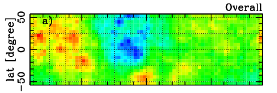
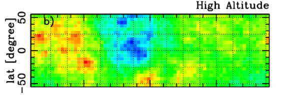
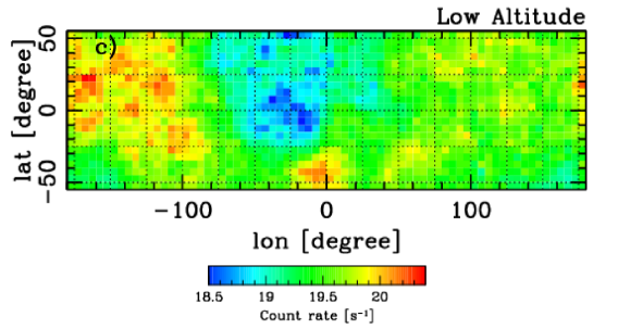
Figure 3: Fiducial states adopted in this article. a) Overall data. b) High Altitude. c) Low-Altitude. The data is pixellized in 5^∘$\times$ 5^∘ bins.

$cr(\mathbf{x,t})$ and $cr_{f}(\mathbf{x})$ are pixellated in 5^∘$\times$ 5^∘ bins: $cr(\mathbf{x}_{ij},t_{k})$ and $cr_{f}(\mathbf{x}_{ij})$, where the spatial coordinate $\mathbf{x}$ is partitioned in latitude $i\in\{1,\cdots,36\}$ and longitude $j\in\{1,\cdots,72\}$, while the two-hour local time bins are represented by $k\in\{1,\cdots,12\}$. In Figure 4 we present the averaged overcount rate, $\langle\delta cr(\mathbf{x}_{ij},t_{k})\rangle_{ij}$, in two-hour local time bins centered around $t_{k}$

$$\langle\delta cr(\mathbf{x}_{ij},t_{k})\rangle_{ij}\equiv\frac{1}{n_{\mbox{\scriptsize{pixels}}}(t_{k})}\sum_{ij}\delta cr(\mathbf{x},t_{k})W(\mathbf{x}_{ij}),$$ (2)

where $\langle\cdots\rangle_{ij}$ denotes the average over all the pixels at a given instant $t_{k}$, the sum is over all the spatial pixels ($i$, $j$), $W(\mathbf{x}_{ij})$ is a spatial “mask” applied to the data as the means to exclude the polar regions:

$$W(\mathbf{x}_{ij})=\left\{\begin{array}[]{ll}1,&\mbox{at latitudes}\in[-55^{\circ},55^{\circ}],\\ \\ 0,&\mbox{everywhere else,}\end{array}\right.$$ (3)

and

$${n_{\mbox{\scriptsize{pixels}}}(t_{k})}\equiv\sum_{ij}W(\mathbf{x}_{ij}).$$ (4)

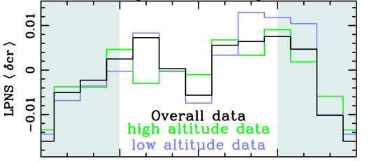
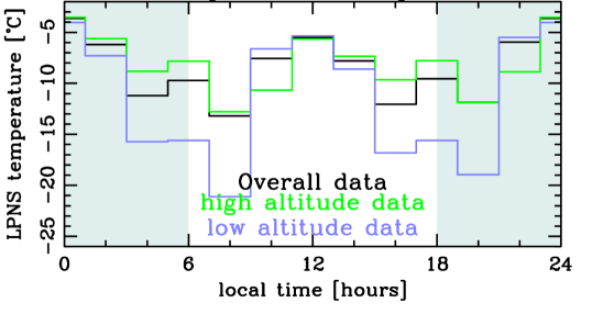
Figure 4: Upper panel Average overcount rate per local time bin. The fiducial map is the mean counting rate at a given location over all the time series. The random errors in the measurements are smaller than 2.1$\times$10^-4, 5.2 $\times$10^-4, 3.5$\times$10^-4 for the overall (black), high altitude (green) and low-altitude (violet) data, respectively. Lower panel Average NS temperature per local time bin. The random errors in the measurements are smaller than 3.4$\times$10^-2, 8.2 $\times$10^-2, 5.2$\times$10^-4 ${{}^{\circ}}C$ for the overall (black), high altitude (green) and low-altitude (violet) data, respectively. The shaded regions of the diagrams represent the nightside. The $x$-axis tickmarks coincide with the local time bin centers.

The three derived time series (overall, high and low-altitude) show significant peak-to-peak variations, $\sim 0.0273$, given that the random errors are smaller than $3.0\times 10^{-4}$.

In principal, these epithermal-neutron local-time variations may be due to variations in bulk hydrogen concentrations across the lunar surface, which is an idea suggested by Livengood et al. [2014] to explain similar variations in LRO/LEND data. However, a comparison of LPNS and LEND data argue against such an interpretation. Specifically, even though the magnitude of the LPNS and LEND local-time variations are similar (2.7% for LPNS versus  2% for LEND), their qualitative behavior is fundamentally different. The LEND data show a single maxima (6 local time [LT]) and minima (15 LT), whereas the LPNS data show two maxima (7 LT and 15 LT) and minima (12 LT and 24 LT). If there were true local-time hydrogen variations that caused a 2 to 2.7% variation in epithermal-neutron count rates, the measured local-time behavior should be similar in both datasets. The fact that their local-time behavior is different suggests that other non-hydrogen systematic variations may be responsible for the observed local-time variations. Because the two sets of measurements were made with different instruments on different spacecraft, such non-hydrogen variations need not be identical in both datasets. Here, we investigate possible sources of non-hydrogen systematic variations in the LPNS data. If we can show that such systematic effects can account for all or most of the local-time variations, then we can conclude that varying hydrogen concentrations are not the cause of these variations. Below, we discuss two such systematic effects: variations in LPNS sensor temperature and variations in lunar surface and subsurface temperatures.

3.1 Epithermal-neutron count rate dependence on LPNS sensor temperature

We first investigate if there is evidence that LPNS sensor temperatures might be related to systematic variations in the epithermal-neutron count rate that have not yet been removed in the prior data reduction procedures [Maurice et al., 2004]. Specifically, we examine if the varying sensor temperatures are related to gain variations (or a multiplicative shift) in the neutron sensor pulse height spectra. If such gain variations exist, we then ask if such variations are related to the  2.7% count rate variations. We note that the variations in the high and low-altitude data are qualitatively similar, so unless otherwise noted, we hereafter only carry out analyses for the low-altitude LPNS data.

Inspection of Figures 1c and 1d shows there is a likely correlation between the sensor temperature and the gain. Figure 5 (upper) shows this correlation explicitly, where the temperature versus peak-channel position for the low-altitude data is plotted. It is clear that the gain of the sensor shows a positive, but non-linear variation with sensor temperature. The dynamic range of the variation is about 0.5 to 0.7 channels, or a 2 to 3% variation.

To investigate if such a gain change could cause a count rate variation of 1 to 2%, Figure 5 (lower) shows a summed pulse height spectrum from the Cd ³He sensor. The LPNS pulse-height spectra were measured with 32 channels, so with such data it is difficult to see if a 0.5 channel difference in gain could cause a counting rate shift. We therefore fit the spectra with a gaussian plus polynomial between channels 10 and 30 and plotted the function using 300 channel values instead of 32 (red dashed line). To simulate the effect of a temperature dependent gain-shift, we shifted the spectra using the largest possible peak-position ratio allowed by the data (25.0/24.3). Both the original and gain shifted spectra are shown in dashed lines (original in red; gain shifted in blue). When one sums the counts between channels 15 and 30 (which are the channels used by Maurice et al. [2004] for the count rate change measurements), there is a 0.7% counting rate change. While this count rate change is smaller than the measured change, it is in the same direction as the measured data, such that lower gain data (which corresponds to lower instrument temperature) shows a larger counting rate, and therefore demonstrates that a varying gain caused by a varying temperature can result in varying LPNS epithermal-neutron count rates.

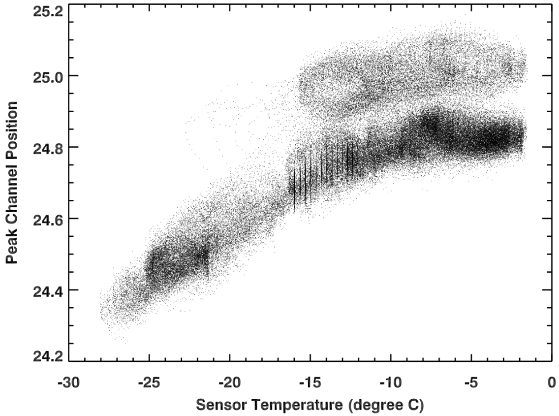
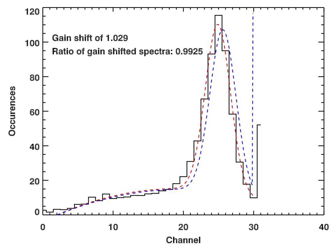
Figure 5: Upper panel Low-altitude Peak-channel Position versus instrumental temperature. Lower panel. Pulse height vs Channel from the LP Cd³He sensor. Original and gain shifted spectra are denoted in dashed lines: original in red and gain shifted in blue (see text for details).

3.2 Neutron Spectrometer sensor temperature correction

To remove the sensor temperature induced count rate variation, we have implemented the following two-step procedure: i) find the linear correlation coefficient between low-altitude time-series count rates and their associated sensor temperatures, and ii) use the linear relationship between those two variables to “de-trend” the data. A least squares fit to the data produces

$$cr=-0.0194\cdot T_{\scriptsize{sensor}}+19.170,$$ (5)

where the sensor temperature, $T_{\scriptsize{sensor}}$, is expressed in ${}^{\circ}C$ and the measured count rate, $cr$, in $s^{-1}$. This relationship is applied to produce the sensor temperature-corrected count rates,

$$cr^{\prime}\equiv cr+0.0194\cdot\left(T_{\scriptsize{sensor}}-\bar{T}_{\scriptsize{sensor}}\right),$$ (6)

where $\bar{T}_{\scriptsize{sensor}}$ denotes the mean sensor temperature. These corrected count rates lead to fluctuations in the low-altitude overcount rates that are reduced from 2.73% to 1.60%, as shown in Table 3 and the violet line in the upper panel of Figure 6. In the same panel of Figure 6 we also present the uncorrected data (green).

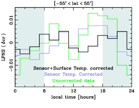
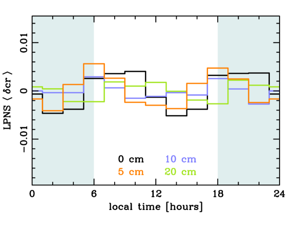
Figure 6: Low-altitude count rate versus local time. Upper panel Black denotes the uncorrected count rate while violet and green represent sensor temperature corrected and sensor plus surface corrected, respectively. Lower panel Subsurface temperature corrected count rates. Black, orange, violet and green represent count rate data corrected with Diviner subsurface temperature models at 0, 5, 10 and 20 cm, respectively. The random errors in all the measurements are smaller than 3.4$\times$10^-4.

Soil type	$a_{soil}$	$b_{soil}$
FAN	20.80	0.00280
Lunar 20 (L20)	20.70	0.00220
Apollo 11 (A11)	20.40	0.00160
Apollo 12 (A12)	20.08	0.00211
Lunar 24 (L24)	19.97	0.00163

Table 1: Various soil parameters, $(a_{soil},b_{soil})$, considered in this work. These parameters were obtained using a linear least squares fit to the points in panel a) of Figure 7. For further details regarding these soils see Lawrence et al. [2006].

3.3 Count rate correlation with lunar surface and subsurface temperature

Little et al. [2003] and Lawrence et al. [2006] used the Monte Carlo transport code MCNPX to study the transport of neutrons in typical lunar soils and found that thermal and epithermal count rates are dependent on soil temperature. Here, we consider a variety of subsurface temperatures as functions of both latitude and local time, constrained by Diviner measurements [Siegler et al., 2011].

To take into account the effects of the lunar subsurface temperature we consider an “average soil” made up of equal fractions of FAN, Luna 20 (L20), Luna 24 (L24), Apollo 11 (A11) and Apollo 12 (A12). In panel a) of Figure 7 we reproduce some of the Lawrence et al. [2006] results for epithermal-neutron count rates from these lunar soils. The dashed black line represents an “average lunar soil”, with epithermal count rates having a temperature dependence given by

$$cr\equiv\bar{a}_{soil}+\bar{b}_{soil}T_{soil}=20.39+2.068\times 10^{-2}T_{soil},$$ (7)

where the soil temperature $T_{soil}$ is expressed in Kelvin. In Table 1 we present the various soil parameters, $(a_{soil},b_{soil})$, that are used in the calculation of $\bar{a}_{soil}$ and $\bar{b}_{soil}$ of Equation 7. These parameters result from linear least squares fits to the points in panel a) of Figure 7.

(Sub)surface temperatures are derived using the Diviner measurements as well as the models constrained by these measurements shown in Figure 2. To obtain the proper temperatures for an epithermal-neutron temperature correction, we interpolate in local time and latitude at a given depth.

Depth	$a^{\prime}_{depth}$	$b^{\prime}_{depth}$
0 cm	19.46	0.00036
1 cm	19.38	0.00067
2 cm	19.19	0.00143
3 cm	18.98	0.00227
4 cm	18.98	0.00227
5 cm	18.84	0.00284
10 cm	18.88	0.00266
20 cm	19.67	-0.00056
30 cm	19.46	0.00036

Table 2: Equation 8 linear least squares fit parameters, $(a^{\prime}_{depth},b^{\prime}_{depth})$, at the various depths used to model the epithermal count rates versus soil temperature.

We fit a linear curve to the box-smoothed count rates versus (sub)surface temperature at various depths, such that

$$cr^{\prime}_{depth}=a^{\prime}_{depth}+b^{\prime}_{depth}T_{soil,\,depth},$$ (8)

where $T_{{{soil,\,depth}}}$ is expressed in Kelvin. The values of $a^{\prime}_{depth}$ and $b^{\prime}_{depth}$ for the various depths are shown in Table 2. In panel b) of Figure 7 we show the count rates corrected for instrumental temperature, $cr^{\prime}$, versus (sub-)surface temperatures at various depths. The count rates are box-smoothed using the same number of observations per bin and are denoted by dotted lines. The corresponding solid lines represent the linear least squares fits at each depth. For the sake of the temperature corrections, the given depth represents the “effective” depth from which the neutrons are emitted and is an approximation to the actual scenario where detected neutrons are emitted from a distribution of depths.

To match the “average lunar soil” count rate versus soil temperature predictions shown at the upper panel of Figure 7 and the LPNS-Diviner measurements of the same relationship shown at the lower panel of the same figure we introduce the following transform:

$$cr_{final,\,depth} = cr^{\prime}_{depth}+$$ (9)

$$\left(\bar{a}_{soil}-a^{\prime}_{depth}\right)+\bar{T}_{soil,\,depth}\left(b^{\prime}_{depth}-\bar{b}_{soil}\right)+$$

$$\left(\bar{b}_{soil}-b^{\prime}_{depth}\right)\left(T_{soil,\,depth}-\bar{T}_{soil,\,depth}\right).$$

Here, $\bar{T}_{soil,\,depth}$ is the average soil temperature at a given depth. Briefly, the transform is made up of two parts: i) move the measured point linear upwards is such a way that makes it coincide with the value of the model predictions at $\bar{T}_{soil,\,depth}$ (second and third terms of the rhs in the above equation), and ii) make the slope of the linear fit to the measured points match the model counterpart, which is denoted by the last term in Equation 9.

In the upper panel of Figure 6 we show the average overcount rate, $\langle\delta cr\rangle$, corrected for sensor temperature and surface temperature effects (black). In the lower panel of the same figure we show the overcount rate as corrected for subsurface temperatures at different depths. Table 3 contains the peak-to-peak variation of the overcount rate for different subsurface temperature corrections, with the minimum variation occurring for the subsurface depth of 20 cm. This result shows that if we correct the LPNS epithermal-neutron count rates for temperature at an effective depth of 20 cm, we can minimize the local-time variations. Because the remaining variation is quite small ($<$0.5%), we therefore find that there is no need to invoke local-time varying hydrogen concentrations to explain most of the LPNS local-time epithermal-neutron variations. We further note that Little et al. [2003] predicted that the “effective” depth for thermal-neutron emission is 30 g/cm², which for a soil density of 1.5 g/cm³, results in a physical depth of 20 cm. This is the same value as our data-constrained effective depth for epithermal-neutrons, and supports the interpretation that much of the measured local-time neutron variations are caused by subsurface temperature variations.

Figure 7: Panel a) This panel, as in Lawrence et al. [2006], shows count rates versus surface temperatures. Each color denotes a different soil: FAN (brown), Lunar 20 (L20, powder green), Apollo 11 (A11, orange), Apollo (A12, violet) and Lunar 24 (L24, blue navy). The dashed black line denotes the “average lunar soil”. Panel b) The measured count rates versus surface and sub-subsurface temperature. Dotted lines represent the box-smoothed count rates. Solid lines denote the least squares fits to the smoothed data. For clarity the 5, 10 and 20 cm curves are shifted upwards by 0.25, 0.50 and 0.75 $s^{-1}$, respectively.

LPNS
sub-dataset	$\left<\delta cr\right>_{\scriptsize{min}}$	$\left<\delta cr\right>_{\scriptsize{max}}$	$\Delta cr$
Overall	-0.0160	0.0075	0.0235
High altitude	-0.0134	0.0091	0.0226
Low-altitude	-0.0144	0.0130	0.0273
Low-altitude
sensor temperature
corrected	-0.0075	0.0075	0.0150
Low-altitude
subsurface
temperature
corrected
Depth 0 cm	-0.0052	0.0040	0.0092
Depth 1 cm	-0.0044	0.0048	0.0092
Depth 2 cm	-0.0053	0.0044	0.0098
Depth 3 cm	-0.0056	0.0052	0.0108
Depth 4 cm	-0.0056	0.0052	0.0108
Depth 5 cm	-0.0042	0.0057	0.0098
Depth 10 cm	-0.0028	0.0029	0.0057
Depth 20 cm	-0.0027	0.0022	0.0049
Depth 30 cm	-0.0052	0.0040	0.0092

Table 3: Peak-to-peak variation of the LPNS overcount rate variation, $\Delta cr\equiv\langle\delta cr\rangle_{\scriptsize{min}}-\langle\delta cr\rangle_{\scriptsize{min}}$, of the different datasets applied in this article.

4 Discussion and Conclusions

In the prior section, we have shown that the LPNS epithermal-neutron count rate data equatorward of 55^∘ show a local-time variation that has a magnitude of 2.7%. We have found that corrections for varying LPNS sensor temperatures and lunar subsurface temperatures can reduce this 2.7% variation to less than 0.5%. Livengood et al. [2014] have also found $\sim$2% local-time variations in the LEND epithermal-neutron count rates. Their interpretation of this result was that these variations were cause by mobile hydrogen that deposits once the sun sets, since the surficial temperature is low enough to lead to a long residence time during the night. It then leaves the lunar surface at dawn as higher temperatures imply very short residence times [see Schörghofer and Taylor, 2007] for a definition of residence time and its dependence on temperature). Because we can quantitatively account for all but 0.5% of the LPNS local-time variation, we find little-to-no support for the interpretation that varying hydrogen concentrations are the dominant cause of the local-time epithermal-neutron variations in either the LPNS or LEND datasets.

Even though the remaining LPNS local-time variations do not exhibit the time dependence expected for diurnal variations suggested by Livengood et al. (2014), we can nevertheless investigate the implications if the remaining 0.5% local-time variations are due to time-variable hydrogen concentrations. Specifically, if a 0.5% diurnal change in epithermal-neutron counting rate were the result of mobile water molecules, then how much water would this imply? We note that for this type of diurnally varying water, the water stratigraphy would likely take the form of a thin wet layer over a thicker dry layer. In this case, we use results from Lawrence et al. [2011] who modeled epithermal-neutron count rates for wet-over-dry layering and found that for top layers thinner than 5 to 10 cm, increasing amounts of hydrogen would result in a epithermal-neutron count rate increase rather than decrease. Here, we therefore assume that hydrogen-bearing compounds are in an upper layer of limited thickness that participates in the diurnal condense/release cycle. We consider Figure 3 of Lawrence et al. [2011] and posit an upper, exchangeable regolith layer thickness of 3 g/cm2. The epithermal count rate in LPNS would increase by $\sim$0.5% if that upper layer contained $\sim$1 wt% water-equivalent hydrogen, i.e., 0.03 g/cm² of H₂O, over dry regolith. This 30 mg/cm² of exchangeable H₂O corresponds to 0.03/18 moles/cm² of H₂O molecules, or 10²¹ molecules/cm². If exchangeable and mobile, this number is the column density of exospheric water that would be present over the dayside. Assuming a rough dayside scale height of 100 km (10⁷ cm), the near-surface density of H₂O would be 10¹⁴ molecules/cm³. Preliminary reports show that observed levels of H₂O and OH are at least 10 orders of magnitude below this value [Benna et al., 2014]). Other mobility scenarios that do not involve the lunar exosphere seem highly implausible.

Alternatively, we suggest that the remaining 0.5% variation is likely to due other systematic variations that have not been fully taken into account. As one suggestion, we consider the fact that the subsurface temperature correction approximated a distribution of neutron emission depths using a single “effective” neutron emission depth. While calculating the true distribution of neutron emission depths is beyond the scope of this current study, we can carry out a slightly more complicated (and possibly realistic) subsurface temperature correction by assuming that the neutrons are uniformly emitted throughout the top 30 cm. With this assumption, we can reduce the prior 0.49% local-time variation to less than 0.25%. While this final result should be treated with some caution because a true depth-dependent emission function has not been derived, it does demonstrate that the remaining 0.49% variation shown in Table 3 can likely be reduced further without appealing to varying hydrogen concentrations.

In summary, we have shown that the LPNS epithermal-neutron data do exhibit local-time variations that have a magnitude of 2.7%. However, these variations can be understood as being due to systematic variations of the LPNS sensor temperature as well as lunar subsurface temperatures. An additional result of this work is that by showing the LPNS local-time variations can be minimized by a subsurface temperature at a depth of 20 cm, the LP neutron data have shown to be consistent with modeled subsurface temperatures, neutron-transport modeled temperature dependencies, as well as the predicted effective depth of subsurface neutron emission.

Acknowledgments
This work was primarily supported by a grant from the NASA Lunar Advanced Science and Exploration Research program to JHU/APL (NNX13AJ61G), and also received support from the NASA Solar System Exploration Research Virtual Institute. VRE was supported by the Science and Technology Facilities Council (UK) [ST/L00075X/1].

References

References

- Benna et al. [2014] M. Benna, T. Stubbs, P. Mahaffy, R. Hodges, D. Hurley, and R Elphic. Ladee nms observations of sporadic water and carbon dioxide in the lunar exosphere. In P21F-02 of AGU Fall Meeting 2014 Abstracts, 2014.
- Eke et al. [2009] V. R. Eke, L. F. A. Teodoro, and R. C. Elphic. The spatial distribution of polar hydrogen deposits on the Moon. Icarus, 200:12–18, March 2009. doi: 10.1016/j.icarus.2008.10.013.
- Elphic et al. [1998] R. C. Elphic, D. J. Lawrence, W. C. Feldman, B. L. Barraclough, S. Maurice, A. B. Binder, and P. G. Lucey. Lunar Fe and Ti Abundances: Comparison of Lunar Prospector and Clementine Data. Science, 281:1493, September 1998. doi: 10.1126/science.281.5382.1493.
- Elphic et al. [2000] R. C. Elphic, D. J. Lawrence, W. C. Feldman, B. L. Barraclough, S. Maurice, A. B. Binder, and P. G. Lucey. Lunar rare earth element distribution and ramifications for FeO and TiO2: Lunar Prospector neutron spectrometer observations. Journal of Geophysical Research, 105:20333–20346, 2000. doi: 10.1029/1999JE001176.
- Feldman et al. [1993] W. C. Feldman, W. V. Boynton, and D. M. Drake. Planetary neutron spectroscopy from orbit. In C. M. Pieters and P. A. J. Englert, editors, Remote Geochemical Analysis, Elemental and Mineralogical Composition, ISBN 0521402816, Cambridge University Press, 1993., 1993.
- Feldman et al. [1998] W. C. Feldman, S. Maurice, A. B. Binder, B. L. Barraclough, R. C. Elphic, and D. J. Lawrence. Fluxes of Fast and Epithermal Neutrons from Lunar Prospector: Evidence for Water Ice at the Lunar Poles. Science, 281:1496–+, September 1998. doi: 10.1126/science.281.5382.1496.
- Feldman et al. [2004] W. C. Feldman, K. Ahola, B. L. Barraclough, R. D. Belian, R. K. Black, R. C. Elphic, D. T. Everett, K. R. Fuller, J. Kroesche, D. J. Lawrence, S. L. Lawson, J. L. Longmire, S. Maurice, M. C. Miller, T. H. Prettyman, S. A. Storms, and G. W. Thornton. Gamma-Ray, Neutron, and Alpha-Particle Spectrometers for the Lunar Prospector mission. Journal of Geophysical Research (Planets), 109:E07S06, July 2004. doi: 10.1029/2003JE002207.
- Heiken et al. [1991] G. Heiken, D. Vaniman, and B.M. French. Lunar Sourcebook: A User’s Guide to the Moon. Cambridge University Press, 1991. ISBN 9780521334440. URL http://books.google.com/books?id=7Q49AAAAIAAJ.
- Lawrence et al. [2006] D. J. Lawrence, W. C. Feldman, R. C. Elphic, J. J. Hagerty, S. Maurice, G. W. McKinney, and T. H. Prettyman. Improved modeling of Lunar Prospector neutron spectrometer data: Implications for hydrogen deposits at the lunar poles. Journal of Geophysical Research (Planets), 111(E10):8001–+, August 2006. doi: 10.1029/2005JE002637.
- Lawrence et al. [2011] D. J. Lawrence, D. M. Hurley, W. C. Feldman, R. C. Elphic, S. Maurice, R. S. Miller, and T. H. Prettyman. Sensitivity of orbital neutron measurements to the thickness and abundance of surficial lunar water. Journal of Geophysical Research (Planets), 116:E01002, January 2011. doi: 10.1029/2010JE003678.
- Lawrence et al. [2015] D. J. Lawrence, P. N. Peplowski, J. B. Plescia, B. T. Greenhagen, S. Maurice, and T. H. Prettyman. Bulk Hydrogen Abundances in the Lunar Highlands: Measurements from Orbital Neutron Data. Icarus (in press), 2015. doi: 10.1016/j.icarus.2015.01.005.
- Little et al. [2003] R. C. Little, W. C. Feldman, S. Maurice, I. Genetay, D. J. Lawrence, S. L. Lawson, O. Gasnault, B. L. Barraclough, R. C. Elphic, T. H. Prettyman, and A. B. Binder. Latitude variation of the subsurface lunar temperature: Lunar Prospector thermal neutrons. Journal of Geophysical Research (Planets), 108:5046, May 2003. doi: 10.1029/2001JE001497.
- Livengood et al. [2014] T. A. Livengood, G. Chin, R. Z. Sagdeev, I. G. Mitrofanov, W. V. Boynton, L. G. Evans, M. L. Litvak, T. P. McClanahan, A. B. Sanin, and R. D. Starr. Evidence for Diurnally Varying Hydration at the Moon’s Equator from the Lunar Exploration Neutron Detector (LEND). In Lunar and Planetary Science Conference, volume 45 of Lunar and Planetary Science Conference, page 1507, March 2014.
- Maurice et al. [2004] S. Maurice, D. J. Lawrence, W. C. Feldman, R. C. Elphic, and O. Gasnault. Reduction of neutron data from Lunar Prospector. Journal of Geophysical Research (Planets), 109:E07S04, June 2004. doi: 10.1029/2003JE002208.
- Schörghofer and Taylor [2007] N. Schörghofer and G. J. Taylor. Subsurface migration of H2O at lunar cold traps. Journal of Geophysical Research (Planets), 112:E02010, February 2007. doi: 10.1029/2006JE002779.
- Siegler et al. [2011] M. A. Siegler, B. G. Bills, and D. A. Paige. Effects of orbital evolution on lunar ice stability. Journal of Geophysical Research (Planets), 116:E03010, March 2011. doi: 10.1029/2010JE003652.
- Sunshine et al. [2009] J. M. Sunshine, T. L. Farnham, L. M. Feaga, O. Groussin, F. Merlin, R. E. Milliken, and M. F. A’Hearn. Temporal and Spatial Variability of Lunar Hydration As Observed by the Deep Impact Spacecraft. Science, 326:565–, October 2009. doi: 10.1126/science.1179788.
- Teodoro et al. [2010] L. F. A. Teodoro, V. R. Eke, and R. C. Elphic. Spatial distribution of lunar polar hydrogen deposits after KAGUYA (SELENE). Geophys. Res. Lett., 37:L12201, June 2010. doi: 10.1029/2010GL042889.
- Teodoro et al. [2014] L. F. A. Teodoro, V. R. Eke, R. C. Elphic, W. C. Feldman, and D. J. Lawrence. How well do we know the polar hydrogen distribution on the Moon? Journal of Geophysical Research (Planets), 119:574–593, March 2014. doi: 10.1002/2013JE004421.