Power law inflation with a non-minimally coupled scalar field in light of Planck and BICEP2 data: The exact versus slow roll results

Abstract

We study power law inflation in the context of non-minimally coupled to the scalar curvature. We analyze the inflationary solutions under an exact analysis and also in the slow roll approximation. In both solutions, we consider the recent data from Planck and BICEP2 data to constraint the parameter in our model. We find that the slow roll approximation is disfavored in the presence of non-minimal couplings during the power law expansion of the Universe.

I Introduction

It is well known that the inflationary scenario has been an important contribution to the modern cosmology, it was particularly successful to explain cosmological puzzles such as the horizon, flatness etc. guth ; linde1983 . As well, the inflationary phase of the Universe provides an elegant mechanism to elucidate the large-scale structureest , and also the detected anisotropy of the cosmic microwave background (CMB) radiationCMB .

On the other hand, the inflationary scenario is supposed to be driven by a scalar field, and also this field can interact fundamentally with other fields, and in particular with the gravity. In this form, is normal to incorporate an explicit non-minimal coupling between the scalar field and the gravitational sector. The non-minimal coupling with the scalar Ricci, was in the beginning considered in radiation problems in Ref.rad , and also in the renormalization of the quantum fields in curved backgrounds, see Refs.r1 ; r2 . It is well known, that scalar fields coupled with the curvature tensor arise in different dimensions Capozziello:2011et , and their importance on cosmological scenarios was studied for first time in Ref.Jor , together with Brans and Dicke BD , although also early the non-minimal coupling of the scalar field was analyzed in Ref.B1 . In the context of the inflationary Universe, the non-minimal coupling has been considered in Refs.val ; fakir ; faraoni , and several inflationary models in the literature Amendola:1999qq ; Uzan:1999ch . In particular, Fakir and Unruh considered a new approach of the chaotic model from the non-minimal coupling to the scalar curvature. Also, in Ref.futamase considered the chaotic potential $V\approx\varphi^{n}$ $(n>4)$ for large $\varphi$ in the context to non-minimal coupling, and found different constraints on the parameter of non-minimal coupling $\xi$ (see also Ref.Bb2 ). Recently, the consistency relation for chaotic inflation model with a non-minimal coupling to gravity was studied in Ref.new1 , and also a global stability analysis for cosmological models with non-minimally coupled scalar fields was considered in Ref.new2 .

On the other hand, in the context of the exact solutions, it can be obtained for instance from a constant potential, “ de Sitter” inflationary modelguth . Similarly, an exact solution can be found in the case of intermediate inflation modelint , however this inflationary model may be best considered from slow-roll analysis. In the same way, an exact solution during inflation can be achieved from an exponential potential during “power-law” inflation in the case of General Relativity. During the power law inflation, the scale factor is given by $a(t)\propto t^{p}$, where the constant $p>1$ pl . In the context of power law inflation with non-minimal coupling has been studied in Refs.futamase ; faraoni . For power law inflation with an effective potential $V\propto\varphi^{n}$ with $n>6$, was analyzed in Ref.faraoni . For this inflationary model, it can be found that only a very small range of the values of the parameter $\xi$ is allowed for high values of the parameter $n$ (see also Refs.chino ; Tsujikawa:2000tm ). Also, Futamase and Maeda futamase considered a chaotic inflationary scenario in models having non-minimal coupling with curvature in the context of power law inflation.

The main goal of the present work is to analyze the possible actualization of an expanding power law inflation within the framework of a non-minimal coupling with curvature, and how the exact and slow roll solutions works in this theory. We shall resort to the BICEP2 experiment data B2 and the Planck satelliteAde:2013uln to constrain the parameters in both solutions. In particular, we obtain constraints on the fundamental coefficients in our model.

The outline of the article is as follows. The next section presents the basic equations and the exact and slow roll solutions for our model. In Sect. III we determine the corresponding cosmological perturbations. Finally, in Sect. IV we summarize our finding. We chose units so that $c=\hbar=1$.

II Basic equations and exact versus slow roll solutions

We start with the action for non-minimal coupling to gravity in the Jordan frame fakir2

$$S=\int d^{4}x\sqrt{-g}\left[\left(\frac{1}{16\pi G}+\frac{1}{2}\xi\varphi^{2}\right)R+\frac{1}{2}g^{\mu\nu}\varphi_{;\mu}\varphi_{;\nu}-V(\varphi)\right],$$ (1)

where $G$ is the Newton‘s gravitational constant, $\xi$ is a dimensionless coupling constant, $R$ is the Ricci scalar and $V$($\varphi$) is the effective potential associated to the scalar field $\varphi$. In particular, for the value of the coupling constant $\xi=0$ corresponds to the minimal coupling, and for the specific case in which $\xi=1/6$ is related to as conformal coupling because the classical action possesses conformal invariance. Also, different constraints on the parameter $\xi$ can be found in the table of Ref.table .

From the action given by Eq.(1), the dynamics in a spatially flat Friedmann-Robertson- Walker (FRW) cosmological model, is described by the equations

$$H^{2}=\frac{8\pi G}{3(1+8\pi G\xi\varphi^{2})}\left[\frac{1}{2}\dot{\varphi}^{2}+V-6\xi H\varphi\dot{\varphi}\right],$$ (2)

$$\dot{H}=-\frac{8\pi G}{1+8\pi G\xi\varphi^{2}}\left[\left(\frac{1}{2}+\xi\right)\dot{\varphi}^{2}-\xi(H\varphi\dot{\varphi}-\varphi\ddot{\varphi})\right],$$ (3)

and

$$V_{,\,\varphi}=6\xi\varphi(\dot{H}+2H^{2})-3H\dot{\varphi}-\ddot{\varphi},$$ (4)

where $H=\dot{a}/a$ is the Hubble parameter and $a$ the scale factor of the FRW metric. Dots means derivatives with respect to time and $V_{,\,\varphi}=\partial V(\varphi)/\partial\varphi$.

In order to obtain an exact solution, we will assume the power law inflation, where the scale factor is characterized by $a\propto t^{p}$, in which $p>1$. Here, the Hubble parameter $H=\dot{a}/a$ is given by $H(t)=p/t$.

Replacing the scale factor $a\propto t^{p}$ in the Eqs.(2)-(4), we find an exact solution for the scalar field, $\varphi$, given by

$$\varphi(t)=b\,t^{n}-\gamma,$$ (5)

where $b$, $n$ and $\gamma$ are constants. For an exact solution of the scalar field, $\gamma$ is defined as

$$\gamma^{2}=-\frac{1}{8\pi G\xi}=-\frac{m_{p}^{2}}{\xi},$$ (6)

where $m_{p}$ is the reduced Planck mass and is defined as $m_{p}^{2}=(8\pi G)^{-1}$. Also, in the following we will consider only negative value of the parameter $\xi$ .

In order to obtain an exact solution, then the relations between $p$ and $\xi$ with the exponent $n$ of Eq.(5), are given by

$$p=\frac{n^{2}-n}{2+n},$$ (7)

and

$$\mid\xi\mid=\frac{(2+n)n}{2[n^{2}+3n-1]}.$$ (8)

Here, we note that the exponent $n$ of the solution of the scalar field given by Eq.(5), is such that, $n\neq-2$, $n\neq(-3-\sqrt{13})/2\approx-3.3$ and $n\neq(-3+\sqrt{13})/2\approx 0.3$. Considering that $p>1$, we note from Eq.(7), that the value of the parameter $n$, becomes $-2<n<1-\sqrt{3}\approx-0.73$ and $n>1+\sqrt{3}\approx 1.73$. In order to obtain the real roots of Eq. (8), we considering only the value of $n<0$. In this form, we find that range for the parameter $\xi$ is given by

$$-\frac{1}{4+\sqrt{3}}<\xi<0.$$ (9)

The Hubble parameter as a function of the scalar field from Eq.(5), becomes

$$H(\varphi)=p\,b^{\frac{1}{n}}(\varphi+\gamma)^{\frac{-1}{n}}.$$ (10)

From Eqs.(2) and (5), the scalar potential as function of the scalar field results

$$V(\varphi)=b^{\frac{2}{n}}(\varphi+\gamma)^{1-\frac{2}{n}}(A\varphi-\gamma B),$$ (11)

where the constants $A$ and $B$ are given by

$$A\equiv-3\mid\xi\mid p(p+2n)-\frac{n^{2}}{2},$$ (12)

and

$$B\equiv-3\mid\xi\mid p^{2}+\frac{n^{2}}{2}.$$ (13)

From Eq.(11) we observe that the effective potential is $V\neq 0$ for the value of $\varphi=0$, since $V(0)=-Bb^{\frac{2}{n}}\gamma^{2-\frac{2}{n}}$. However, we note that the constant $B$ is negative from the range of the parameter $\xi$, see Eq.(9) , and then the effective potential becomes $V(\varphi=0)>0$ (see Refs.hosotani ; faraoni for other $V(0)\neq 0$).

In order to reproduce the present value of the Newton’s gravitational constant, we can write from Ref.futamase , that $G_{eff}=\frac{G}{1-\frac{\varphi^{2}}{\gamma^{2}}}$. Here, $G_{eff}$ corresponds to the effective Newton’s gravitational constant. By considering that $G_{eff}>0$, we observe that the scalar field is well supported by the condition $\mid\varphi\mid<\frac{m_{p}}{\sqrt{\mid\xi\mid}}=\gamma$, then the inflationary scenario can be realized in the region in which $-\gamma\lesssim\varphi\lesssim\gamma$.

In the following, we will study the power law solution in the slow roll conditions. Following Ref. Torres:1996fr the slow roll approximation are defined as $\dot{H}\ll H^{2}$ and $\ddot{\varphi}\ll 3H\dot{\varphi}$. In this form, the slow roll field equations from Eqs.(2)-(4) can be written as

$$H^{2}\simeq\frac{8\pi G}{3(1+8\pi G\xi\varphi^{2})}(V(\varphi)-6\xi H\varphi\dot{\varphi}),$$ (14)

and

$$3H\dot{\varphi}+V_{,\,\varphi}\simeq 12\xi\varphi\,H^{2}.$$ (15)

Considering the power law expansion $a\propto t^{p}$, we get

$$\varphi(t)=bt^{-2}-\gamma,$$ (16)

with

$$p=\frac{2}{\mid\xi\mid}-4>1,$$

where the constant $\gamma$ as before is given by Eq.(6), and during the slow roll approximation the value of $|\xi|<2/5$. As before, since the Hubble parameter is $H\propto t^{-1}$, we can eliminate $t$ by using Eq.(16), thus $H(\varphi)=pb^{-1/2}(\varphi+\gamma)^{1/2},$ and the effective potential results

$$V(\varphi)=3pb^{-1}\mid\xi\mid(\varphi+\gamma)^{2}[\gamma p+\varphi(4-p)].$$ (17)

Here, we note that in the slow roll approximation, the solution for the scalar field is $\varphi\propto t^{-2}$ (with the fixed value $n=-2$, see Eq.(5)), and also the exact effective potential reduces to the cubical polynomial form as potential given by Eq.(17).

III Cosmological perturbations

In this section we will analyze the scalar and tensor perturbations for our model. The general perturbation metric about the flat background is given by

$$ds^{2}=-(1+2\Phi)dt^{2}+2a(t)\Theta_{,i}dx^{i}dt+a^{2}(t)[(1-2\psi)\delta_{ij}+2E_{,i,j}+2h_{ij}]dx^{i}dx^{j},$$ (18)

where $\Phi$, $\Theta$, $\psi$ and $E$ represent to the scalar-type metric perturbations, and the tensor $h_{ij}$ corresponds the transverse traceless perturbation.

On the other hand, the perturbation in the scalar field $\varphi$ is specified as $\varphi(t,\vec{x})=\varphi(t)+\delta\varphi(t,\vec{x})$, where $\varphi(t)$ is the background scalar field that satisfies the Eq.(4), and $\delta\varphi(t,\vec{x})$ is a small perturbation that represents small fluctuations of the corresponding scalar field. In this form, we introduce comoving curvature perturbations, given by Bardeen

$${\cal{R}}=\Psi+\mathcal{H}\frac{\delta\varphi}{\varphi^{\prime}}\;,$$ (19)

where now the Hubble parameter is defined as $\mathcal{H}\equiv\frac{a^{\prime}}{a}$ and a prime denotes a derivative with respect to a conformal time $d\eta=a(t)^{-1}dt$.

From the action given by Eq.(1), we find that the perturbed equations of motion are given by

$$\Psi^{\prime}+\mathcal{H}\Phi=\frac{1}{2F}(f^{\prime}-\Phi F^{\prime}-\mathcal{H}f+\varphi^{\prime}\delta\varphi),$$ (20)

$$\Psi-\Phi=\frac{f}{F},$$ (21)

and

$$3\mathcal{H}^{2}f+2F(\nabla^{2}\Psi-3\mathcal{H}[\Psi^{\prime}+\mathcal{H}\Phi])=-3\mathcal{H}f^{\prime}+3F^{\prime}\Psi^{\prime}+\nabla^{2}f+\varphi^{\prime}\delta\varphi^{\prime}$$ (22)

$$-\Phi\varphi^{\prime 2}+6\Phi\mathcal{H}F^{\prime}+a^{2}V_{,\varphi}\delta\varphi,$$

where $F=F(\varphi)=(8\pi G)^{-1}+\xi\varphi^{2}$ and $f=\delta F=(\partial F/\partial\varphi)\delta\varphi$. Also, we considering the longitudinal gauge in the perturbed metric (18), where $\Phi=\Phi(t,\vec{x})$ and $\Psi=\Psi(t,\vec{x})$ are gauge-invariant variables introduced in Ref.Bardeen .

Defining two auxiliary functions; $\alpha=\frac{3F^{\prime 2}}{2F}+\varphi^{\prime 2}$ and $\beta=\mathcal{H}+\frac{F^{\prime}}{2F}$, then using Eq.(19), the equations (20), (21), and (22) can be written in the form

$${\cal{R}}^{\prime}+A_{1}\delta\varphi+B_{1}\delta\varphi^{\prime}+\beta{\cal{R}}=0,$$ (23)

and

$$C\delta\varphi^{\prime}-6F\beta{\cal{R}}^{\prime}+\frac{CA_{1}}{B_{1}}\delta\varphi-C\varphi^{\prime}{\cal{R}}+2F\nabla^{2}{\cal{R}}+2FB_{1}\nabla^{2}\delta\varphi=0,$$ (24)

where $A_{1}$, $B_{1}$ and $C$ are given by $A_{1}=\frac{\beta\varphi^{\prime\prime}}{\varphi^{\prime 2}}-\frac{2\beta^{2}}{\varphi^{\prime}}$ , $B_{1}=-\frac{\beta}{\varphi^{\prime}}$ and $C=\frac{1}{\varphi^{\prime}}(6F\beta^{2}-\alpha)$, respectively.

Following Ref.noh , the Eqs.(23) and (24) can be decoupled, and then the equation of motion for the curvature perturbation becomes

$$\frac{1}{a^{3}Q_{s}}\frac{d}{dt}{(a^{3}Q_{s}\dot{{\cal{R}}})}+\frac{k^{2}}{a^{2}}{\cal{R}}=0,\,\,\,\,\,\,\mbox{with}\,\,\,\,\,Q_{s}\equiv\frac{\alpha}{\beta^{2}},$$ (25)

where $k$ is a comoving wavenumber. Here, we note that the equation for the curvature perturbation given by Eq.(24), coincides with the equation obtained in Ref.hwang . Introducing new variables, in which $z=a\sqrt{Q_{s}}$ and $v=a{\cal{R}}$, the above equation can be written as $v^{\prime\prime}+(k^{2}-\frac{z^{\prime\prime}}{z})v=0$, see Ref.shinji .

As argued in Refs.noh ; shinji , the solution of the above equation can be expressed by the combination of the Hankel function, and the scalar density perturbation ${\cal{P}}_{S}$, could be written as

$${\cal{P}}_{S}\equiv\frac{k^{3}}{2\pi^{2}}|{\cal{R}}|^{2}=A_{S}^{2}\left[\frac{k|\eta|}{2}\right]^{3-2\nu_{s}},$$ (26)

where $A_{S}^{2}\equiv\frac{1}{Q_{s}}(\frac{H}{2\pi})^{2}(\frac{1}{aH|\eta|})^{2}[\frac{\Gamma(\nu_{s})}{\Gamma(3/2)}]^{2}$ and $\nu_{s}\equiv\sqrt{\gamma_{s}+1/4}$. Here, $\gamma_{s}$ is defined as

$$\gamma_{s}=\frac{(1+\delta_{s})(2-\epsilon+\delta_{s})}{(1-\epsilon)^{2}},\,\,\,\,\,\mbox{where}\,\,\,\;\delta_{s}\equiv\frac{\dot{Q_{s}}}{2HQ_{s}},\,\,\,\mbox{and}\,\,\,\epsilon\equiv-\frac{\dot{H}}{H^{2}}\,.$$

The scalar spectral index $n_{S}$ is given by $n_{S}-1=\frac{d\ln{\cal{P_{S}}}}{d\ln k}$. From Eq.(26), it follows that shinji

$$n_{S}=4-\sqrt{4\gamma_{s}+1}.$$ (27)

The spectrum of tensor perturbations, $h_{ij}$ can be obtained in a similar way, since $h_{ij}$ satisfies the equivalent form of Eq.(25). In this form, following Ref.shinji in the which $Q_{s}\to Q_{T}=F$, the power spectrum of the tensor modes ${\cal{P}}_{T}$, can be written as

$${\cal{P}}_{T}\equiv A_{T}^{2}\left[\frac{k|\eta|}{2}\right]^{3-2\nu_{T}},$$ (28)

where $A_{T}^{2}\equiv\frac{8}{Q_{T}}(\frac{H}{2\pi})^{2}(\frac{1}{aH|\eta|})^{2}[\frac{\Gamma(\nu_{T})}{\Gamma(3/2)}]^{2}$, and the parameters $\nu_{T}$, $\gamma_{T}$ and $\delta_{T}$ are given by

$$\nu_{T}\equiv\sqrt{\gamma_{T}+1/4},\,\,\,\gamma_{T}=\frac{(1+\delta_{T})(2-\epsilon+\delta_{T})}{(1-\epsilon)^{2}},\,\,\,\mbox{and}\,\,\,\delta_{T}=\frac{\dot{Q}_{T}}{2HQ_{T}}.$$

Here, the index of the tensor perturbation is given by ${n}_{T}=3-\sqrt{4{\gamma}_{T}+1}$.

On the other hand, an essential observational quantity is the tensor to scalar ratio $r$, which is defined as $r={\cal{P}}_{T}/{\cal{P}}_{S}$. In this way, combining Eqs.(26) and (28) the tensor to scalar ratio is given by

$$r=8\frac{Q_{s}}{Q_{T}}\left[\frac{\Gamma(\nu_{T})}{\Gamma(\nu_{s})}\right]^{2}=8\left[\frac{\frac{3F^{\prime 2}}{2F}+\varphi^{\prime 2}}{F(\mathcal{H}+\frac{F^{\prime}}{2F})^{2}}\right]\left[\frac{\Gamma(\nu_{T})}{\Gamma(\nu_{s})}\right]^{2}.$$ (29)

In this form, considering the power law inflation, i.e., $a\propto t^{p}$, and the exact solution for the scalar field given by Eq.(5), then the scalar spectral index $n_{s}$ as a function of the scalar field $\varphi$ can be written as

$$n_{S}(\varphi)-1=3-\sqrt{4\gamma_{s}(\varphi)+1},$$ (30)

where $\gamma_{s}(\varphi)$ is given by

$$\gamma_{s}(\varphi)=p\,\left[\frac{(1+\delta_{s}(\varphi))\,(2p-1+p\delta_{s}(\varphi))}{(p-1)^{2}}\right],$$

with

$$\delta_{s}(\varphi)=\frac{n}{p}\left[1+(\gamma-\varphi)^{-1}\left(\frac{6m_{p}^{2}\gamma^{2}\varphi}{\varphi^{2}(6m_{p}^{2}-\gamma^{2})+\gamma^{4}}+\frac{n\gamma(\varphi+\gamma)}{p\gamma-\varphi(p+n)}\right)\right].$$

Also, the tensor to scalar ratio $r$ can be written in terms of the scalar field $\varphi$ as

$$r(\varphi)=\frac{8n^{2}}{m_{p}^{2}}\left(\frac{\varphi^{2}(6m_{p}^{2}-\gamma^{2})+\gamma^{4}}{(p\gamma-\varphi(p+n))^{2}}\left[\frac{\Gamma(\nu_{T})}{\Gamma(\nu_{s})}\right]^{2}\right).$$ (31)

Here, we have considered Eqs.(5) and (29).

In the slow-roll approximation, following Ref.shinji , the scalar spectral index is given by

$$n_{S}-1\approx-2(\delta_{s}+\epsilon),$$ (32)

and the tensor to scalar ratio $r$ becomes

$$r\approx 16\left(\frac{\dot{F}}{2HF}+\epsilon\right),$$ (33)

because during the slow roll approximation, $\mid\delta_{s}\mid<1$ and $\mid\delta_{T}\mid<1$. Also, here we considered that $\Gamma(\nu_{s})\simeq\Gamma(\nu_{T})\simeq\Gamma(3/2)$, since that both perturbations are close to scale invariant shinji , see also Refs.noh ; kaiser .

Under the slow roll approximation the quantity $\delta_{s}$ is given by

$$\delta_{s}=\frac{\mid\xi\mid}{2|\xi|-1}\left[1+(\gamma-\varphi)^{-1}\left(\frac{6m_{p}^{2}\gamma^{2}\varphi}{\varphi^{2}(6m_{p}^{2}-\gamma^{2})+\gamma^{4}}-\frac{\mid\xi\mid\gamma(\varphi+\gamma)}{(1-2|\xi|)[\gamma-\varphi]+|\xi|\varphi}\right)\right].$$

Here, we have considered the slow-roll solution for the scalar field given by Eq.(16).

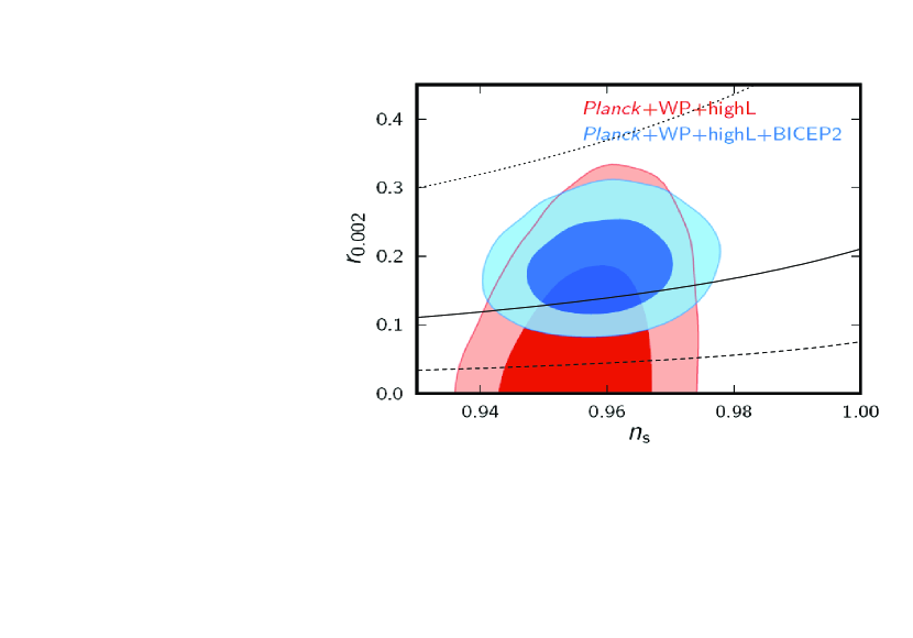
Figure 1: Evolution of the tensor-scalar ratio $r$ versus the scalar spectrum index $n_{s}$, from the exact solution for three different values of the parameter $\xi$. The dotted, solid , and dashed lines are for the $\mid\xi\mid\simeq 0.10$, $\mid\xi\mid\simeq 0.08$ and $\mid\xi\mid\simeq 0.06$, respectively.

In Fig.(1) we show the evolution of the tensor-to-scalar ratio $r$ on the scalar spectral index $n_{S}$ for three different values of $\xi$. Dotted, solid , and dashed lines are for the $\mid\xi\mid\simeq 0.10$, $\mid\xi\mid\simeq 0.08$ and $\mid\xi\mid\simeq 0.06$, respectively. Here, we note that for the value of $\mid\xi\mid\simeq 0.10$ corresponds to $n=-1.59$ (or equivalently $\varphi\propto t^{-1.59}$) and $p=10.04$ (or equivalently $a\propto t^{10.04}$), see Eqs.(7) and (8). Analogously, for the value of $\mid\xi\mid\simeq 0.08$ corresponds to $n=-1.7$ and $p=15.3$ and for the value of $\mid\xi\mid\simeq 0.06$ corresponds to $n=-1.8$ and $p=25.2$.

In this plot we show the two-dimensional marginalized constraints, at 68$\%$ and 95$\%$ levels of confidence, for the tensor-to-scalar ratio and the scalar spectral index (considered BICEP2 experiment data B2 in connection with Planck + WP + highL). In order to write down values for the tensor-to-scalar ratio and the scalar spectral index, we numerically obtain the parametric plot of the consistency relation $r=r(n_{S})$ considering Eqs.(30) and (31), obtained from the exact solution for the scalar field given by Eq.(5).

From this plot we find that the range for the parameter $0.08\lesssim|\xi|\lesssim 0.10$ (or equivalently $-1.7\lesssim n\lesssim-1.59$ and $10.04\lesssim p\lesssim 15.3$ ), which is well supported from BICEP2 experiment. For values of $|\xi|<0.08$ the model is rejected from BICEP2, because $r=0.2_{-0.05}^{+0.07}$, and also $r=0$ disproved at $7.0\sigma$. Nevertheless, from Planck satellite and other CMB experiments generated exclusively an upper limit for the tensor -to- scalar ratio $r$, where $r<0.11$ (at 95$\%$ C.L.)Ade:2013uln . Recently, the Planck Collaboration has made out the data concerning the polarized dust emissionAdam:2014bub . From an analysis of the polarized thermal emissions from diffuse Galactic dust in different range of frequencies, indicates that BICEP2 gravitational wave data could be due to the dust contamination. Here, an elaborated study of Planck satellite and BICEP2 data would be demanded for a definitive answer. In this way, we numerically find that the parameter $|\xi|\lesssim 0.10$ is well supported by Planck satellite. Here, we note that this constraint of $\xi$ negative is similar to found in Ref.table , where an effective potential $V\propto\varphi^{4}$ has been studied.

On the other hand, considering the slow roll approximation for the consistency relation $r=r(n_{s})$ from Eqs.(32) and (33), we observe that the slow roll model is disproved from observations; because the spectral index $n_{S}>1$, and then the model does not work from the slow roll analysis (figure not shown). Here, we noted that $\delta_{s}<0$, and then the spectral index $n_{S}$ during the slow roll approximation becomes $n_{S}>1$.

IV Conclusions

In this paper we have studied the power law inflation in the context of a non-minimally coupled scalar field. From the equations of motion and also in the slow roll approximation we have found exact and slow roll solutions for our model, during the power law expansion. In our model, we have obtained analytical expression for the corresponding effective potential, power spectrum, scalar spectrum index, and tensor- to-scalar ratio considering the exact solutions and slow roll analysis. From these measures, we have found constraint on the parameter $|\xi|$ (or equivalently $n$ and $p$) from BICEP2 experiment and Planck data, where we have studied the constraint on the consistency relation $r=r(n_{s})$.

From the exact solution we have found a constraint for the value of the parameter $|\xi|$. In this form, from BICEP2 we have obtained an upper bound and a lower bound for the parameter $|\xi|$ given by $0.08\lesssim|\xi|\lesssim 0.10$ (or equivalently $-1.7\lesssim n\lesssim-1.59$ and $10.04\lesssim p\lesssim 15.3$ ). However, we have found that the parameter $|\xi|\lesssim 0.10$ is well supported by Planck data and other CMB experiments. Finally, we have observed during the slow-roll approximation, the model is disproved by observations, being that the spectral index $n_{S}>1$, and the model does not work from slow roll analysis.

- (1) A. H. Guth, Phys. Rev. D 23, 347 (1981)
- (2) A.Linde, Phys. Lett. B 129, 177 (1983)
- (3) V.F. Mukhanov and G.V. Chibisov , JETP Letters 33, 532(1981). 20; S. W. Hawking,Phys. Lett. B 115, 295 (1982); A. Guth and S.-Y. Pi, Phys. Rev. Lett. 49, 1110 (1982); A. A. Starobinsky, Phys. Lett. B 117, 175 (1982); J.M. Bardeen, P.J. Steinhardt and M.S. Turner, Phys. Rev.D28, 679 (1983).
- (4) D. Larson et al., Astrophys. J. Suppl. 192, 16 (2011); C. L. Bennett et al., Astrophys. J. Suppl. 192, 17 (2011); G. Hinshaw et al. [WMAP Collaboration], Astrophys. J. Suppl. 208, 19 (2013).
- (5) N.A. Chernikov.; E.A.Tagirov, Quantum theory of scalar field in de Sitter space. Ann. Inst. H. Poincare A 9, 1091¤71411 (1968).
- (6) C.G. Callan; S.Coleman.; R.Jackiw. A new improved energy-momentum tensor. Ann. Phys. 59, 421¤773 (1970).
- (7) Birrell, N.D.; Davies, P.C. Quantum Fields in Curved Space; Cambridge University Press: Cambridge, UK, 1980; Nelson, B.; Panangaden, P. Scaling behavior of interacting quantum fields in curved spacetime. Phys. Rev. D25, 10191¤71027 (1982).
- (8) S. Capozziello and M. De Laurentis, Phys. Rept. 509, 167 (2011); K. Nozari and N. Rashidi, Phys. Rev. D 86 043505 (2012).
- (9) P. Jordan, Z. Phys. 157, 112 (1959).
- (10) C. Brans and R.H. Dicke, Phys. Rev. 124, 925 (1961).
- (11) N.A. Chernikov and E.A. Tagirov, Ann. Inst. H. Poincare A 9, 109 (1968); C.G. Callan Jr., S. Coleman and R. Jackiw, Ann. Phys. (NY) 59, 42 (1970).
- (12) V. Faraoni, Phys. Rev. D62 023504 (2000); V. Faraoni, E. Gunzig and P. Nardone, Fund. Cosmic Phys. 20, 121 (1999); E.Komatsu and T. Futamase, Phys.Rev. D59 064029 (1999).
- (13) R.Fakir and W G Unruh, Astrophys. J, 394 396 (1992).
- (14) V. Faraoni, Phys. Rev. D 53, 6813 (1996); J. R. Morris, Class. Quant. Grav. 18, 2977 (2001).
- (15) J. P. Uzan, Phys. Rev. D 59, 123510 (1999); A. A. Starobinsky, S. Tsujikawa and J. Yokoyama, Nucl. Phys. B 610, 383 (2001).
- (16) L. Amendola, Phys. Rev. D 60, 043501 (1999).
- (17) T. Futamase and K. Maeda, Phys. Rev. D 39, 399 (1989).
- (18) N. Makino and M. Sasaki, Prog. Theor. Phys. 86, 103 (1991); T. Futamase, T. Rothman and R. Matzner, Phys. Rev. D 39, 405 (1989); E. Komatsu and T. Futamase, Phys. Rev. D 58, 023004 (1998). [Erratum-ibid. D 58, 089902 (1998)]; E. Komatsu and T. Futamase, Phys. Rev. D 59, 064029 (1999).
- (19) T. Chiba and K. Kohri, arXiv:1411.7104 [astro-ph.CO].
- (20) M. A. Skugoreva, A. V. Toporensky and S. Y. Vernov, Phys. Rev. D 90, 064044 (2014).
- (21) J. D Barrow, Phys. Lett. B235, 40 (1990).
- (22) F. Lucchin and S. Matarrese, Phys. Rev. D32, 1316 (1985).
- (23) Chen Shi-Wu et al. Chinese Phys. Lett. 25, 3162 (2008).
- (24) S. Tsujikawa, Phys. Rev. D 62, 043512 (2000).
- (25) P. A. R. Ade et al. [BICEP2 Collaboration], Phys. Rev. Lett. 112, 241101 (2014); P. A. R. Ade et al. [BICEP2 Collaboration], Astrophys. J. 792, 62 (2014).
- (26) P. A. R. Ade et al. [Planck Collaboration], Astron. Astrophys. 571, A22 (2014).
- (27) R.Fakir and W.G. Unruh, Phys. Rev. D 41, 1783 (1990).
- (28) K. Nozari and S. D. Sadatian, Mod. Phys. Lett. A 23, 2933 (2008).
- (29) Y. Hosotani, Phys. Rev. D 32, 1949 (1985).
- (30) D. F. Torres, Phys. Lett. A 225, 13 (1997).
- (31) J. Bardeen, Phys. Rev. D 22, 1882 (1980).
- (32) H.Noh and J.Hwang, Phys.Lett. B515, 231-237 (2001).
- (33) J. Hwang, Phys.Rev. D53, 762-765 (1996).
- (34) S.Tsujikawa and B.Gumjudpai, Phys.Rev.D69, 123523 (2004).
- (35) D. Kaiser, Phys. Rev. D 81, 084044 (2010).
- (36) R. Adam et al. [Planck Collaboration], arXiv:1409.5738 [astro-ph.CO].