Joint Channel Direction Information Quantization For Spatially Correlated 3D MIMO Channels

Abstract

This paper proposes a codebook for jointly quantizing channel direction information (CDI) of spatially correlated three-dimensional (3D) multi-input-multi-output (MIMO) channels. To reduce the dimension for quantizing the CDI of large antenna arrays, we introduce a special structure to the codewords by using Tucker decomposition to exploit the unique features of 3D MIMO channels. Specifically, the codeword consists of four parts each with low dimension individually targeting at a different type of information: statistical CDIs in horizontal direction and in vertical direction, statistical power coupling, and instantaneous CDI. The proposed codebook avoids the redundancy led by existing independent CDI quantization. Analytical results provide a sufficient condition on 3D MIMO channels to show that the proposed codebook can achieve the same quantization performance as the well-known rotated codebook applied to the global channel CDI, but with significant reduction in the required statistical channel information. Simulation results validate our analysis and demonstrate that the proposed joint CDI quantization provides substantial performance gain over independent CDI quantization.

I Introduction

To meet the ever-growing data demand in future 5th Generation (5G) cellular networks, one of the promising ways is to increase the number of antennas at the base station (BS) [1]. However, equipping large number of antennas at a BS is challenging due to the physical space limitation. This naturally calls for three-dimensional (3D) multi-input-and-multi-output (MIMO) systems [2, 3, 4, 5], where active antenna elements are placed in a two-dimensional (2D) array, e.g., rectangular and circular arrays, or even non-planar arrays, at the BS.

The non-linear arrays can provide both horizonal and vertical spatial resolution, and thus can support 3D beamforming [3]. 3D beamforming can be user-specific, which improves the signal to noise ratio (SNR) meanwhile generating less interference to adjacent users. Recently, a 3D MIMO prototype system operating at millimeter-wave bands was reported to support a multi-Gbps data rate service in macro cells, which provides high array gain to compensate the severe path loss [5].

In practice, the promised performance of 3D beamforming largely depends on how accurate the channel direction information (CDI) is obtained at the BS. In time division duplexing (TDD) systems, the CDI obtained by channel estimation in uplink can be used for beamforming in downlink if the antennas at the BS are perfectly calibrated [1], where the performance is limited by pilot contamination [6]. In frequency division duplexing (FDD) systems, limited feedback is widely used, where the CDI is firstly quantized at the user and then fed back to the BS [7]. Yet the feedback overhead is supposed to increase with the number of antennas [8], which is not acceptable for large antenna array systems.

Spatial correlation is observed very typical in MIMO channels [9], due to small spacing between adjacent antennas and low angular spreads. In [10], B. Clerckx, et al. found that spatial correlation can be exploited to reduce the overhead for feeding back CDI significantly. The same conclusion was drawn in [11, 12, 13] for spatially correlated massive MIMO channels, which indicates that FDD is also applicable for large antenna array systems without heavy feedback overhead as supposed to be.

Various codebooks have been proposed for spatially correlated channels. Theoretically, Llyod algorithm [14] can be applied to generate codebooks for 3D MIMO channels, but they are difficult to be used off-line in practice. There are some codebooks obtained from Llyod algorithms with reduced complexity, e.g., local-packing codebook [15], and gain and phase separated quantization [16]. A well-known codebook, rotated codebook [17], transforms the codewords optimized for uncorrelated channels (e.g., Grassmannian subspace packing (GSP) codewords) by channel correlation matrix. It was proved that the rotated codebook is asymptotically optimal in quantizing any spatially correlated channels as the codebook size becomes large [18]. An extension of rotated codebook to multiuser MIMO system is provided in [19], where not only each user’s own but also the other users’ correlation matrices are employed for the codeword rotation. When designing codebooks for real-world cellular systems, practical limitations such as constant modulus and finite alphabet need to be taken into account. Discrete Fourier transformation (DFT) codebook meets these limitations, which is suitable for highly correlated channels with uniform linear array at the BS [20]. For 3D MIMO system with uniform rectangular array (URA), a Kronecker-product DFT codebook was proposed in [21]. However, as shown in [20], the performance of these pure DFT based codebooks degrades severely when the angular spreads of channel increase.

Generally speaking, there are two straightforward strategies to extend existing codebooks to 3D MIMO systems. The first strategy is global channel quantization, which expresses the 3D MIMO channel as a larger global vector, and reuse existing codebooks proposed for 2D MIMO channels. For example, the codebooks in [17, 15, 16, 22] can be applied to quantize the global 3D MIMO CDI directly. However, due to the high dimension of the resulting CDI vector, it is challenging for the BS to obtain accurate channel statistical information required by the global channel quantization to reuse existing codebooks, e.g., channel correlation matrix used by the rotated codebook, which is known as the “curse of the dimensionality” [23]. Moreover, large dimension incurs high complexity in matrix operations [24]. The second strategy is independent CDI quantization, which quantizes the CDI of 3D MIMO in horizontal and vertical directions independently and reuses existing codebooks in each direction [4]. This strategy is simple and avoids the problem caused by the high dimensional channel vector, which however comes at a cost of low quantization accuracy when the angular spread is large, as will be clarified later.

To design a desirable codebook in 3D MIMO channels under various angular spreads and reduce the amount of required spatial correlation information, we propose a joint CDI quantization strategy to quantize the CDI of two directions jointly. The designed codeword has a special structure led by the Tucker decomposition [25], which exploits the unique features of 3D MIMO channels.

The first feature of 3D MIMO channel is the inherent geometrical structure inherited from the regularity of antenna arrays. For example, the array response of 3D MIMO with URA for each ray in the channel can be decomposed into two subarray responses of lower channel dimensions in horizontal and vertical directions. Similar decompositions can be also found for those large arrays nested from several smaller identical subarrays. This feature can be exploited for coping with the high-dimension quantization problem in large antenna arrays.

The second feature is power coupling. When the array responses of 3D MIMO channels are decomposed into two subarray responses respectively in horizontal and vertical directions, a common ray gain is shared by the two subarray responses and not decomposable. The power coupling is important in the codebook design, since it connects with the subarray responses from different lower channel dimensions. The feature can be exploited to avoid the redundancy in the CDI quantization.

Although many research efforts have been made for the dimension reduction problem, they mainly employ the singular value decomposition (SVD) of correlation matrix to exploit the channel correlation, e.g., [26]. As far as the authors known, the unique features in 3D MIMO channels are not yet exploited. In this paper, we propose a codebook for jointly quantizing the CDIs in horizontal and vertical directions, where a new codeword structure is introduced to reduce the dimension by using the features of 3D MIMO channels. The contributions are two-fold:

1. A joint CDI quantization codebook is proposed to quantize spatially correlated 3D MIMO channels, which has a special codeword structure. The spatial correlation information required by the cobook for general antenna arrays is provided by using the Tucker decomposition. We show that the proposed codebook provides better quantization performance than the independent CDI quantization, and requires much less spatial correlation information than the globally rotated codebook.

2. The performance of joint CDI quantization codebook is analyzed. We show that the performance is the same as the globally rotated codebook for 3D MIMO systems with URA under the channels with weak identically independent distributed (i.i.d.) rays.

The rest of this paper is organized as follows. In Section II, we present the 3D MIMO channel model and channel representations. In Section III, we propose the joint CDI quantization codebook for spatially correlated channels. In Section IV, a solution to find the spatial correlation information for general antenna arrays is provided by using the Tucker decomposition. The performance of the joint CDI quantization codebook is analyzed in Section V. Simulation results are provided in Section VI and the paper is concluded in Section VII.

Notations: $(\cdot)^{T}$, $(\cdot)^{H}$ and $(\cdot)^{\ast}$ are respectively the transpose, Hermitian and conjugate operation, $\odot$ and $\otimes$ are respectively the element-wise and Kronecker matrix product, $|\cdot|$ and $\|\cdot\|$ are respectively the absolute value and norm, $\boldsymbol{E}\{\}$ means the expectation operation, $\text{diag}(\boldsymbol{x})$ is the diagonal matrix with diagonal entries given in the vector $\boldsymbol{x}$, and $\text{diag}(\boldsymbol{X})$ is the diagonal matrix with the diagonal equal to that of the matrix $\boldsymbol{X}$.

II System and Channel Models

Consider a downlink 3D MIMO system where an array with $N_{t}$ antennas is mounted at the BS [27, 2], and all antennas are omni-directional. An example of 3D MIMO system with URA is shown in Fig. 1.

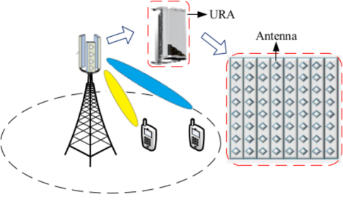
Figure 1: An example of 3D MIMO system with $8\times 8$ URA at the BS.

For easy exposition, we start by considering the 3D multiple-input-and-single-output (MISO) system with single-antenna users, and then extend the design to multi-antenna users. For simplicity, we will not distinguish 3D MISO channel from 3D MIMO channel hereafter.

According to the generic spatial channel modeling methods [28, 9, 29], the 3D MIMO channel consists of several scattering clusters distributed in the 3D space, where in each cluster there are multiple rays with small random angle offsets, which can be expressed as a $N_{t}$-dimensional vector

$$\boldsymbol{h} \triangleq\sum\nolimits_{n=1}^{N}\sum\nolimits_{m=1}^{M}g_{n,m}\boldsymbol{a}(\Theta_{n,m})$$ (1)

where $g_{n,m}\in\mathbb{C}$ is the random gain of the $m$th ray in the $n$th cluster with zero mean, the angle vector $\Theta_{n,m}=[\theta_{n,m},\phi_{n,m}]^{T}$ is specified by the angle coordinates $\theta_{n,m}$ and $\phi_{n,m}$ in the 3D space, and $\boldsymbol{a}(\Theta_{n,m})\in\mathbb{C}^{N_{t}\times 1}$ is the corresponding array response.

The expression of array response $\boldsymbol{a}(\Theta_{n,m})$ depends on the specific form of the array mounted at the BS. The array responses of some well-structured arrays can be decomposed into the Kronecker product of subarray responses, while the others may not. Usually, the large antenna arrays nested from smaller identical subarrays are decomposable. For example, as shown in [28, 30], the array response of URA can be decomposed into two subarray responses respectively in horizontal and vertical directions as

$$\boldsymbol{a}(\Theta_{n,m})=\boldsymbol{a}_{v}(\phi_{n,m})\otimes\boldsymbol{a}_{h}(\theta_{n,m})$$ (2)

with

$$\boldsymbol{a}_{h}(\theta_{n,m})\! =\![1,e^{j2\pi\frac{d_{h}}{\lambda}{\cos\theta_{n,m}}},\!\cdots\!,\!e^{j2\pi\frac{d_{h}}{\lambda}(N_{h}-1){\cos\theta_{n,m}}}]^{T}$$

$$\boldsymbol{a}_{v}(\phi_{n,m})\! =\![1,e^{j2\pi\frac{d_{v}}{\lambda}{\cos\phi_{n,m}}},\!\cdots\!,\!e^{j2\pi\frac{d_{v}}{\lambda}(N_{v}-1){\cos\phi_{n,m}}}]^{T}$$

where $d_{h}$ and $d_{v}$ are respectively the antenna spacing in horizontal and vertical directions, $N_{h}$ and $N_{v}$ are the number of antennas at the URA in horizontal and vertical directions, $\lambda$ is the carrier wavelength, $\cos\theta_{n,m}$ and $\cos\phi_{n,m}$ are the direction cosines of the $m$th ray in the $n$th cluster respectively in the horizontal and vertical directions.

One example of non-decomposable array response is the uniform concentric circular array (UCCA). Denote $J$ and $L$ respectively as the number of rings and the number of antennas equally placed on each ring in the array. As shown in [30], the array response of UCCA can be expressed as

$$\boldsymbol{a}(\Theta_{n,m})=[\boldsymbol{a}(\varphi_{1})^{T},\cdots\boldsymbol{a}(\varphi_{L})^{T}]^{T}$$ (3)

with

$$\boldsymbol{a}(\varphi_{l})\! =\![e^{j2\pi\frac{d_{1}}{\lambda}{\cos(\phi_{n,m}-\varphi_{l})\cos\theta_{n,m}}},$$

$$\!\cdots\!,\!e^{j2\pi\frac{d_{J}}{\lambda}{\cos(\phi_{n,m}-\varphi_{l})\cos\theta_{n,m}}}]^{T}$$

where $d_{j}$ and $\varphi_{l}=2l\pi/L$ are respectively the radius of the $j$th ring and the $l$th radial direction in the array, $j=1,\ldots,J$, $l=1,\ldots,L$, $\theta_{n,m}$ and $\phi_{n,m}$ are respectively the directions of the $m$th ray in the $n$th cluster with respect to the positive x- and y-axis in the array.

The CDI of 3D MIMO channel is $\bar{\boldsymbol{h}}={\boldsymbol{h}}/|\boldsymbol{h}|$, which is of unit-norm [7]. In limited feedback MIMO systems, the CDI is quantized at the user by using a pre-determined codebook and then fed back to the BS. The quality of CDI available at the BS largely depends on the codebook. A desirable codebook should be judiciously designed by taking the channel features into account. To observe the unique features of 3D MIMO channels, besides the vector expression $\boldsymbol{h}\in\mathbb{C}^{N_{t}\times 1}$, we also express the channel in matrix form.

Taking the URA as an example, the 3D MIMO channel and the array response can be expressed as

$$\boldsymbol{H}\in\mathbb{C}^{N_{h}\times N_{v}}~{}\text{and}~{}\boldsymbol{A}_{n,m}=\boldsymbol{a}_{h}(\theta_{n,m})\boldsymbol{a}_{v}(\phi_{n,m})^{T}$$ (4)

where $\boldsymbol{h}=\text{vec}(\boldsymbol{H})$, $\boldsymbol{a}(\Theta_{n,m})=\text{vec}(\boldsymbol{A}_{n,m})$, and $\text{vec}(\cdot)$ denotes the operation of vectorizing a matrix into a vector. Then, the CDI can be expressed as $\bar{\boldsymbol{H}}=\boldsymbol{H}/\|\boldsymbol{H}\|$.

The matrix representation helps us to identify the different types of channel information in 3D MIMO channels with the URA, since the columns and rows of $\boldsymbol{H}$ respectively stand for the sub-responses at the horizontal and vertical directions.

If the ray responses of an array are decomposable, i.e., $\boldsymbol{a}(\Theta_{n,m})=\boldsymbol{x}\otimes\boldsymbol{y}$, we can easily find the matrix expression for each array response as $\boldsymbol{x}\boldsymbol{y}^{T}$ and the matrix expression for the channel, where $\boldsymbol{x}$ and $\boldsymbol{y}$ are not necessarily the sub-responses in the horizontal and vertical directions. However, the matrix expressions for arbitrary antenna arrays can not be obtained straightforwardly and will be discussed in Section IV.

III Codebook Design

In this section, we propose a joint quantization codebook for spatially correlated 3D MIMO channels, given that the channel matrix expression $\boldsymbol{H}$ is available.

When tens or hundreds of antennas are placed in the array, say $N_{t}=64$ or $256$, the dimension of vectors $\boldsymbol{a}(\Theta_{n,m})$ and $\boldsymbol{h}$ can be very large, and the dimension of corresponding channel correlation matrix is much larger since

$$\boldsymbol{R}=\boldsymbol{E}\{\boldsymbol{h}\boldsymbol{h}^{H}\}$$ (5)

which is of size $N_{t}\times N_{t}$. In fact, the dimension $N_{t}\times N_{t}$ is large even for small value of $N_{h}$ and $N_{v}$, say $N_{t}=N_{h}N_{v}=8^{2}$ for $N_{h}=N_{v}=8$. Such a large dimension not only increases the computational complexity for MIMO signal processing but also results in the difficultly of CDI feedback [31].

The channel correlation matrix $\boldsymbol{R}$ is important for many codebooks [17, 26, 19]. For example, when $\boldsymbol{R}$ is available, the rotated codebook can immediately be applied to quantize the 3D MIMO CDI vector, $\boldsymbol{\bar{h}}$. Specifically, the globally rotated codeword can be constructed from an instantaneous codeword $\boldsymbol{g}_{0}$ of size $N_{t}\times 1$ as [17]

$$\boldsymbol{c}_{g}=\boldsymbol{R}^{1/2}\boldsymbol{g}_{0}$$ (6)

where the codeword $\boldsymbol{c}_{g}$ is of unit-norm.

The globally rotated codebook has been proved to be asymptotical optimal to quantize arbitrary spatially correlated channels [18]. Yet it is challenging to obtain the channel correlation matrix $\boldsymbol{R}$ at the BS since $N_{t}$ is large in 3D MIMO systems. In the sequel, we strive to reduce the dimension of quantization by exploiting unique features of 3D MIMO channels.

III-A Different Types of CDI of 3D MIMO Channels

We begin with the following proposition to identify different types of CDI in 3D MIMO channels.

Proposition 1

Any 3D MIMO channel matrix $\boldsymbol{H}$ can be decomposed into $\boldsymbol{H}=\boldsymbol{U}_{h}\boldsymbol{H}_{t}\boldsymbol{U}_{v}^{T}$ such that $\boldsymbol{E}\{\boldsymbol{H}_{t}\boldsymbol{H}_{t}^{H}\}=\text{diag}(\boldsymbol{\lambda}_{h})$ and $\boldsymbol{E}\{\boldsymbol{H}_{t}^{T}\boldsymbol{H}_{t}^{\ast}\}=\text{diag}(\boldsymbol{\lambda}_{v})$, where $\boldsymbol{U}_{h}$ and $\boldsymbol{U}_{v}$ are unitary matrices, $\boldsymbol{\lambda}_{h}$ and $\boldsymbol{\lambda}_{v}$ are vectors with nonnegative entries.

Proof: The proposition is easy to show by taking the SVD to channel matrix, which is given here simply for introducing notations.

Denote the SVD of the left and right correlation matrices of 3D MIMO channel respectively as

$$\boldsymbol{R}_{h} ={\boldsymbol{E}}\{\boldsymbol{H}\boldsymbol{H}^{H}\}=\boldsymbol{U}_{h}\text{diag}(\boldsymbol{\lambda}_{h})\boldsymbol{U}_{h}^{H}$$ (7)

$$\boldsymbol{R}_{v} ={\boldsymbol{E}}\{\boldsymbol{H}^{T}\boldsymbol{H}^{\ast}\}=\boldsymbol{U}_{v}\text{diag}(\boldsymbol{\lambda}_{v})\boldsymbol{U}_{v}^{H}$$ (8)

where the entries of $\boldsymbol{\lambda}_{h}$ and $\boldsymbol{\lambda}_{v}$ are in a descending order. Considering that $\boldsymbol{H}_{t}=\boldsymbol{U}_{h}^{H}\boldsymbol{H}\boldsymbol{U}_{v}^{\ast}$, and by using (7) and (8), we can obtain the proposition. $\blacksquare$

This proposition suggests that for arbitrary 3D MIMO systems under arbitrary channels, we can always obtain two unitary matrices shown in (7) and (8). Although this is nothing but taking the SVD to the 3D MIMO channel matrix, but the geometrical structure of the array has been explicitly exploited.

Note that we can also obtain a unitary matrix $\boldsymbol{U}$ for the full channel correlation matrix by the SVD as $\boldsymbol{R}=\boldsymbol{U}\text{diag}(\boldsymbol{\lambda})\boldsymbol{U}^{H}$. To emphasize the difference, the unitary matrix $\boldsymbol{U}$ is referred to as statistical direction information, and the two unitary matrices $\boldsymbol{U}_{h}$, $\boldsymbol{U}_{v}$ are referred to as statistical sub-direction information.

The statistical direction information can transform the 3D MIMO channel matrix $\boldsymbol{H}$ into at most $N_{h}N_{v}$ uncorrelated channel gains expressed in the diagonal matrix $\text{diag}(\boldsymbol{\lambda})$. In contrast, the two statistical sub-direction information independently transform the channel matrix $\boldsymbol{H}$ into at most $N_{h}$ and $N_{v}$ uncorrelated channel gains respectively expressed in diagonal matrices $\text{diag}(\boldsymbol{\lambda}_{h})$ and $\text{diag}(\boldsymbol{\lambda}_{v})$. One desirable property of statistical sub-direction information is that the dimensions of the correlation matrices of $N_{h}\times N_{h}$ and $N_{v}\times N_{v}$ are much smaller than $N_{h}N_{v}\times N_{h}N_{v}$ for statistical direction information. In the sequel, we refer to the two sub-directions as “horizontal” and “vertical” directions, although such notions only agree with their physical meanings for the URA.

Denote $\boldsymbol{\Lambda}_{i,j}$ as the the average channel gain of the $(i,j)$th element in $\boldsymbol{H}_{t}$ given by Proposition 1, e.g., $\boldsymbol{\Lambda}^{2}_{i,j}\!=\!{\boldsymbol{E}}\{|\boldsymbol{H}_{t,i,j}|^{2}\}$. By expressing $\boldsymbol{u}_{i}$ and $\boldsymbol{v}_{i}$ respectively as the $i$th column of matrix $\boldsymbol{U}_{h}$ and $\boldsymbol{U}_{v}$, then $\boldsymbol{\Lambda}_{i,j}$ can be also expressed by

$$\boldsymbol{\Lambda}_{i,j}\!=\!{\boldsymbol{E}}^{\frac{1}{2}}\{|\boldsymbol{u}^{H}_{i}\boldsymbol{H}\boldsymbol{v}^{\ast}_{j}|^{2}\}.$$ (9)

which means $\boldsymbol{\Lambda}_{i,j}$ is the common average channel gain shared by the $i$th statistical horizontal direction and $j$th statistical vertical direction.

Different from $\boldsymbol{\lambda}_{h}$ in (7) and $\boldsymbol{\lambda}_{v}$ in (8) which are obtained separately, $\boldsymbol{\Lambda}$ is interacted jointly with $\boldsymbol{U}_{h}$ and $\boldsymbol{U}_{v}$, and can be interpreted as the statistical power coupling information.

III-B The Proposed Codeword Structure

Based on Proposition 1 and the observations in last subsection, we propose a joint quantization codeword structure for quantizing the CDI of 3D MIMO channel in matrix form, $\bar{\boldsymbol{H}}=\boldsymbol{H}/\|\boldsymbol{H}\|$, by separating the statistical sub-directions, the average and instantaneous channel gains, which is

$$\boldsymbol{C}_{J}=\hat{\boldsymbol{U}}_{h}(\hat{\boldsymbol{\Lambda}}\odot\boldsymbol{G})\hat{\boldsymbol{U}}_{v}^{T}$$ (10)

where the codeword $\boldsymbol{C}_{J}$ is normalized to have unit norm. By using $\text{vec}(ABC^{T})=(C\otimes A)\text{vec}(B)$, the codeword structure for quantizing the CDI of 3D MIMO channel in vector form $\bar{\boldsymbol{h}}$ can be expressed as

$$\boldsymbol{c}_{J}=(\hat{\boldsymbol{U}}_{v}\otimes\hat{\boldsymbol{U}}_{h})\text{diag}(\hat{\boldsymbol{\lambda}})\boldsymbol{g}$$ (11)

where $\boldsymbol{c}_{J}=\text{vec}(\boldsymbol{C}_{J})$, $\hat{\boldsymbol{\lambda}}=\text{vec}(\hat{\boldsymbol{\Lambda}})$ and $\boldsymbol{g}=\text{vec}(\boldsymbol{G})$.

The role of each part of the codeword is as follows,

• unitary matrix $\hat{\boldsymbol{U}}_{h}$ is of size $N_{h}\times r_{h}$, which targets at the statistical sub-direction information $\boldsymbol{U}_{h}$ in horizontal direction ($1\leq r_{h}\leq N_{h}$),

• unitary matrix $\hat{\boldsymbol{U}}_{v}$ is of size $N_{v}\times r_{v}$, which targets at the statistical sub-direction information $\boldsymbol{U}_{v}$ in vertical direction ($1\leq r_{v}\leq N_{v}$),

• nonnegative scaler matrix $\hat{\boldsymbol{\Lambda}}$ is of size $r_{h}\times r_{v}$, which targets at the statistical power coupling information $\boldsymbol{\Lambda}$ between the horizontal and vertical directions,

• instantaneous codeword $\boldsymbol{G}$ is of size $r_{h}\times r_{v}$, which quantizes the instantaneous power coupling information. In fact, the instantaneous power coupling information reflects the instantaneous CDI of $\boldsymbol{H}_{t}$ in Proposition 1.

With the codeword structure in (10), the CDIs in horizontal and vertical directions are jointly quantized together with the power coupling. Therefore, we refer the codebook of codewords with this structure as the joint CDI quantization codebook.

Compared with the codeword structure of the globally rotated codebook shown in (6), the proposed codeword structure in (11) needs low-dimensional statistical channel information for rotation.

In practice, the statistical information $\boldsymbol{U}_{h}$, $\boldsymbol{U}_{v}$ and $\boldsymbol{\Lambda}$ can be obtained at the BS either by uplink channel estimation or by feedback.

In FDD systems where the downlink and the uplink are operated at separated frequency bands, estimating the downlink channel correlation matrix from uplink training symbols is still possible [32]. However, such a method may not be used to estimate the channel correlation matrix $\boldsymbol{R}$ for 3D MIMO systems, which is of high dimension. The problem of estimating the correlation matrix for high-dimension random vectors is recognized as “curse of dimensionality” and far from trivial [24]. This is because the dimension of the channel correlation matrix may be comparable with the number of collected training symbols such that the widely-used “sample covariance” estimation becomes invalid.

The matrices $\boldsymbol{U}_{h}$, $\boldsymbol{U}_{v}$ and $\boldsymbol{\Lambda}$ can also be quantized and fed back [33, 34]. Since the spatial correlation information can be fed back in wide-band and in long-term, the feedback overhead can be almost ignored compared with the feedback for instantaneous CDI. This is especially true when the array feature is taken into account. For example, for the URA, according to Szego’s theory of Toeplitz matrices, the statistical sub-direction information $\boldsymbol{U}_{h}$ and $\boldsymbol{U}_{v}$ become a subset of DFT matrix when the size of the array increases [11]. This will significantly simplify the feedback for the correlation information.

Since our focus is to reduce the dimension of quantization by introducing new codeword structure, we assume that the statistical channel information ${\boldsymbol{U}}_{h}$, ${\boldsymbol{U}}_{v}$ and ${\boldsymbol{\Lambda}}$ are available at the BS. Then, the matrices used to construct the codewod with structure in (10) $\hat{\boldsymbol{U}}_{h}$, $\hat{\boldsymbol{U}}_{v}$ and $\hat{\boldsymbol{\Lambda}}$ can be obtained as

$$\hat{\boldsymbol{U}}_{h} =[\boldsymbol{u}_{1},\cdots,\boldsymbol{u}_{r_{h}}],\quad\hat{\boldsymbol{U}}_{v}=[\boldsymbol{v}_{1},\cdots,\boldsymbol{v}_{r_{v}}]$$

$$\hat{\boldsymbol{\Lambda}}_{i,j} =\boldsymbol{\Lambda}_{i,j},\text{with~{}}1\leq i\leq r_{h},1\leq j\leq r_{v}$$ (12)

The codeword quantizing the instantaneous CDI of 3D MIMO channel, i.e., $\boldsymbol{G}$, can be obtained by using the codebooks designed for uncorrelated channels with dimension of $r_{h}\times r_{v}$. For example, GSP codebooks proposed in [7] can be used, which is optimized for uncorrelated Rayleigh channels.

The dimensions $r_{h}$ and $r_{v}$ in (10) can be designed to further reduce the dimension of codeword by discarding trivial statistical sub-directions in strong correlated channel. We leave this topic for future study, since similar idea has already been developed in [26], and moreover, the dimension parameter can be optimized by considering various system parameters, e.g., the error tolerance, storage space, and overall quantization performance.

III-C Extension to Multi-antenna Users

When considering multiple receive antennas at the user, it is reasonable to assume that the statistical channel information in (10) associated with different receive antennas are identical due to the small space separation. However, the instantaneous CDI associated with different receive antennas may differ. Based on this observation, we can easily extend the codebook design to the systems where each user is equipped with $N_{r}$ antennas.

Denote the super-script in parentheses as the index of receiver antenna, the joint quantization codeword in (11) for multi-antenna users can be given as

$$\boldsymbol{c}_{J}^{(1,\dots,N_{r})}\! =\![\boldsymbol{c}_{J}^{(1)},\!\cdots\!,\!\boldsymbol{c}_{J}^{(N_{r})}]$$

$$\!=(\hat{\boldsymbol{U}}_{v}\otimes\hat{\boldsymbol{U}}_{h}){\text{diag}(\hat{\boldsymbol{\lambda}})}[\boldsymbol{g}^{(1)},\!\cdots\!,\!\boldsymbol{g}^{(N_{r})}]$$

where $\boldsymbol{g}^{(1)},\cdots,\boldsymbol{g}^{(N_{r})}$ are respectively the instantaneous codewords for different receive antennas.

IV Statistical Information for Arbitrary Antenna Array

The proposed codeword structure is applicable for any antenna array if the channel can be expressed in matrix form as $\boldsymbol{H}$. This is because Proposition 1 is valid for arbitrary 3D MIMO channels. Although quite natural to the decomposable arrays such as the URA, the way to express the channels in matrix form for arbitrary antenna array is not obvious because of two issues.

The first issue is the choice of dimensionality for the 3D MIMO channel matrix, i.e., $N_{h}$ and $N_{v}$ with $N_{h}\times N_{v}=N_{t}$. Taking the UCCA array with $N_{t}=32$ as an example, we may express the channel vector $\boldsymbol{h}$ in a matrix form $\boldsymbol{H}$ of size $8\times 4$, $4\times 8$, or the others, but we are not clear which expression achieves a better quantization performance because the array is not rectangular.

The second issue is the “antenna grouping” in the channel matrix, i.e., which subset of antenna responses should be in the same row or column in $\boldsymbol{H}$ for a given dimensionality of $N_{h}$ and $N_{v}$. The antenna grouping determines the values of $\boldsymbol{U}_{h}$, $\boldsymbol{U}_{v}$ and $\boldsymbol{\Lambda}$, and eventually affects the performance of the proposed codebook.

As a consequence, we need to solve these two issues when designing the joint codebook for 3D MIMO systems with arbitrary antenna array. The challenges for addressing the two issues are different. The choices satisfying $N_{t}=N_{h}\times N_{v}$ are always limited, and thus exhaustive searching is efficient to find the best dimensionality. However, the possible choices of antenna grouping exponentially increases with $N_{t}$, which belongs to a combinational problem and is of prohibitive computational complexity. Therefore, we focus on the second issue in the following, i.e., to find proper $\boldsymbol{U}_{h}$, $\boldsymbol{U}_{v}$ and $\boldsymbol{\Lambda}$ for a given $N_{h}$ and $N_{v}$.

IV-A Optimizing $\boldsymbol{U}_{h}$, $\boldsymbol{U}_{v}$ and $\boldsymbol{\Lambda}$

To find the desirable statistical information, before solving the antenna grouping problem, we first reconsider the proposed codebook structure. Recall that the entries of $\boldsymbol{H}_{t}$ defined in Proposition 1 reflect the instantaneous channel gains, and the GSP codebook can be used to quantize the instantaneous CDI, which is optimal for i.i.d. channels. Therefore, the proposed codebook will be optimal if the entries of $\boldsymbol{H}_{t}$ are uncorrelated and the statistical information is perfect (i.e., $\hat{\boldsymbol{U}}_{h}=\boldsymbol{U}_{h}$, $\hat{\boldsymbol{U}}_{h}=\boldsymbol{U}_{v}$ and $\hat{\boldsymbol{\Lambda}}=\boldsymbol{\Lambda}$).

We can reconstruct a full channel matrix $\hat{\boldsymbol{R}}$ from the matrices with lower dimensions as

$$\hat{\boldsymbol{R}} =\boldsymbol{E}\{\text{vec}(\boldsymbol{U}_{h}\boldsymbol{H}_{t}\boldsymbol{U}_{v}^{T})\text{vec}(\boldsymbol{U}_{h}\boldsymbol{H}_{t}\boldsymbol{U}_{v}^{T})^{H}\}$$

$$=(\boldsymbol{U}_{v}\otimes\boldsymbol{U}_{h})\boldsymbol{E}\{\text{vec}\{\boldsymbol{H}_{t}\}\text{vec}\{\boldsymbol{H}_{t}\}^{H}\}(\boldsymbol{U}_{v}\otimes\boldsymbol{U}_{h})^{H}$$

$$=(\boldsymbol{U}_{v}\!\otimes\!\boldsymbol{U}_{h})\text{diag}(\text{vec}\{\boldsymbol{\Lambda}\!\odot\!\boldsymbol{\Lambda}\})(\boldsymbol{U}_{v}\!\otimes\!\boldsymbol{U}_{h})^{H}$$ (13)

where (13) is achieved when the entries of $\boldsymbol{H}_{t}$ are uncorrelated.

If $\hat{\boldsymbol{R}}=\boldsymbol{R}$, the proposed codebook is identical to the globally rotated codebook, since the codeword in (11) becomes $\boldsymbol{c}_{J}=\hat{\boldsymbol{R}}^{\frac{1}{2}}\boldsymbol{g}$ and the same as in (6). Unfortunately, in general cases, $\hat{\boldsymbol{R}}\neq\boldsymbol{R}$, and the proposed codebook becomes inferior to the globally rotated codebook, which is asymptotically optimal. To provide good quantization performance, it is reasonable to find $\boldsymbol{U}_{h}$, $\boldsymbol{U}_{v}$ and $\boldsymbol{\Lambda}$ such that $\hat{\boldsymbol{R}}$ is as close to $\boldsymbol{R}$ as possible.

For simplicity, we define $\boldsymbol{\lambda}_{t}=\text{vec}\{\boldsymbol{\Lambda}\odot\boldsymbol{\Lambda}\}$. The problem of finding the optimal $\boldsymbol{U}_{h}$, $\boldsymbol{U}_{v}$ and $\boldsymbol{\lambda}_{t}$ for arbitrary antenna array can be modeled as

$$\min_{\boldsymbol{U}_{h},\boldsymbol{U}_{v},\boldsymbol{\lambda}_{t}} \|\boldsymbol{R}\!-\!(\boldsymbol{U}_{v}\!\otimes\!\boldsymbol{U}_{h})\text{diag}(\boldsymbol{\lambda}_{t})(\boldsymbol{U}_{v}\!\otimes\!\boldsymbol{U}_{h})^{H}\|^{2}_{F}$$ (14)

s.t. $$~{}~{}\quad\boldsymbol{U}_{v}^{H}\boldsymbol{U}_{v}=\boldsymbol{I}_{N_{v}},$$

$$~{}~{}\quad\boldsymbol{U}_{h}^{H}\boldsymbol{U}_{h}=\boldsymbol{I}_{N_{h}},$$

$$~{}~{}\quad\boldsymbol{\lambda}_{t}\succ 0$$

where $\boldsymbol{I}_{n}$ is the identity matrix of size $n\times n$, and $\boldsymbol{x}\succ 0$ means each element in $\boldsymbol{x}$ is larger than $0$. The problem in (14) does not directly optimize the antenna grouping in the channel matrix, which is unnecessary since when given the optimal solution of $\boldsymbol{U}_{h}$, $\boldsymbol{U}_{v}$ and $\boldsymbol{\lambda}_{t}$, we can obtain the matrices used to construct the joint quantization codewods.

Problem (14) belongs to a classic approximation problem of Tucker decomposition [25], where $\boldsymbol{\lambda}_{t}$ is the core tensor, $\boldsymbol{U}_{h}$ and $\boldsymbol{U}_{v}$ are respectively the factor matrices with columns $\boldsymbol{u}_{i}$ and $\boldsymbol{v}_{i}$ as tensors. The main objective of Tucker decomposition is to decompose a higher dimensional matrix into low dimensional factor matrices, and the tensor core encompass all the possible interactions among the low dimensional tensors in the factor matrices. In other words, Tucker decomposition is to reduce the dimension in the large matrix by finding the structure properties. Moreover, Tucker decomposition is a generation of the matrix SVD with several desirable features, such as orthogonality, decorrelation and computational tractability. However, in general the problem of finding the solution of Tucker decomposition is NP-hard, and there are few efficient algorithms in use.

Note that although the problem in (14) contains three variables, it can be simplified by only optimizing $\boldsymbol{U}_{h}$ and $\boldsymbol{U}_{v}$ without losing the optimality. This is because given $\boldsymbol{U}_{h}$ and $\boldsymbol{U}_{v}$, the objective function satisfies

$$\quad\min_{\boldsymbol{\lambda}_{t}}\|\boldsymbol{R}\!-\!(\boldsymbol{U}_{v}\!\otimes\!\boldsymbol{U}_{h})\text{diag}(\boldsymbol{\lambda}_{t})(\boldsymbol{U}_{v}\!\otimes\!\boldsymbol{U}_{h})^{H}\|_{F}^{2}$$

$$=\min_{\boldsymbol{\lambda}_{t}}\!\|(\boldsymbol{U}_{v}\!\otimes\boldsymbol{U}_{h})^{H}\boldsymbol{R}(\boldsymbol{U}_{v}\!\otimes\!\boldsymbol{U}_{h})\!\!-\!\text{diag}(\boldsymbol{\lambda}_{t})\|_{F}^{2}$$ (15)

$$=\min_{\boldsymbol{\lambda}_{t}}\!\|\text{diag}\left((\boldsymbol{U}_{v}\!\otimes\boldsymbol{U}_{h})^{H}\boldsymbol{R}(\boldsymbol{U}_{v}\!\otimes\!\boldsymbol{U}_{h})\right)\!\!-\!\text{diag}(\boldsymbol{\lambda}_{t})\|_{F}^{2}$$

$$\quad+\|\text{off}\left((\boldsymbol{U}_{v}\otimes\boldsymbol{U}_{h})^{H}\boldsymbol{R}(\boldsymbol{U}_{v}\otimes\boldsymbol{U}_{h})\right)\|_{F}^{2}$$

$$=\|\text{off}\left((\boldsymbol{U}_{v}\otimes\boldsymbol{U}_{h})^{H}\boldsymbol{R}(\boldsymbol{U}_{v}\otimes\boldsymbol{U}_{h})\right)\|_{F}^{2}$$ (16)

where (15) is due to fact that the norm is unitarily invariant, $\text{off}(\boldsymbol{X})$ is the operation to the matrix $\boldsymbol{X}$ with all zeros on the diagonal, (16) is achieved by the optimal $\boldsymbol{\lambda}_{t}$ for a given $\boldsymbol{U}_{h}$ and $\boldsymbol{U}_{v}$, which is

$$\text{diag}(\boldsymbol{\lambda}_{t})=\text{diag}\left((\boldsymbol{U}_{v}\otimes\boldsymbol{U}_{h})^{H}\boldsymbol{R}(\boldsymbol{U}_{v}\otimes\boldsymbol{U}_{h})\right)$$ (17)

It can be verified that the operation for computing $\boldsymbol{\lambda}_{t}$ in (17) is identical to that for computing $\boldsymbol{\Lambda}$ with (9).

Since (16) does not depend on the parameter $\boldsymbol{\lambda}_{t}$, we only need to find $\boldsymbol{U}_{h}$ and $\boldsymbol{U}_{v}$ from a new optimization problem by replacing the objective function in (14) with (16). With the optimized $\boldsymbol{U}_{h}$ and $\boldsymbol{U}_{v}$, we can immediately obtaining optimal $\boldsymbol{\lambda}_{t}$ by using (17).

IV-B Closed-form Solution for $\boldsymbol{U}_{h}$ and $\boldsymbol{U}_{v}$

Since a closed-form solution is more desirable for practical use, we consider a modified problem to find $\boldsymbol{U}_{h}$ and $\boldsymbol{U}_{v}$. Specifically, we impose an extra constraint on $\boldsymbol{\lambda}_{t}$ into the new optimization problem, which is given by

$$\boldsymbol{\lambda}_{t}=\boldsymbol{\lambda}_{v}\otimes\boldsymbol{\lambda}_{h}$$ (18)

where $\boldsymbol{\lambda}_{v}\succ 0$ and $\boldsymbol{\lambda}_{h}\succ 0$. Then, the term inside the objective function of problem (14) becomes

$$\!(\boldsymbol{U}_{v}\!\otimes\!\boldsymbol{U}_{h})\text{diag}(\boldsymbol{\lambda}_{t})(\boldsymbol{U}_{v}\!\otimes\!\boldsymbol{U}_{h})^{H}=\boldsymbol{B}\otimes\boldsymbol{C}$$ (19)

where $\boldsymbol{B}=\boldsymbol{U}_{v}\text{diag}(\boldsymbol{\lambda}_{v})\boldsymbol{U}_{v}^{H}$ and $\boldsymbol{C}=\boldsymbol{U}_{h}\text{diag}(\boldsymbol{\lambda}_{h})\boldsymbol{U}_{h}^{H}$ are positive semi-definite matrices.

With the constraint in (18) and considering (19), the optimization problem to find $\boldsymbol{U}_{h}$ and $\boldsymbol{U}_{v}$ becomes

$$\min_{B,C} ~{}~{}\|\boldsymbol{R}-\boldsymbol{B}\otimes\boldsymbol{C}\|^{2}_{F}$$ (20)

s.t. $$~{}~{}\boldsymbol{B}\in\mathbb{S}^{N_{v}\times N_{v}},\text{and}~{}\boldsymbol{C}\in\mathbb{S}^{N_{h}\times N_{h}}$$

where $\mathbb{S}^{n\times n}$ is the space of positive semi-definite matrices with the dimensionality of $n\times n$.

The new problem in (20) offers a suboptimal solution of $\boldsymbol{U}_{h}$ and $\boldsymbol{U}_{v}$ with closed-form for the Tucker decomposition, and is known as the Kronecker product decomposition [35]. There are many other benefits to consider the Kronecker product decomposition here. By using such an decomposition, many structure properties of $\boldsymbol{R}$, such as symmetry, definite, and permutations, can be inherited by the matrices $\boldsymbol{B}$ and $\boldsymbol{C}$. It is worthy to note that these structure properties are usually led by the regularity of antenna array, e.g., symmetry, and nested subarrays.

The solution to the problem in (20) is given in [35]. To obtain the solution, according to [35], we need to rearrange the matrix $\boldsymbol{R}$. Specifically, the matrix $\boldsymbol{R}$ is divided into $N_{v}\times N_{v}$ blocks as

$$\boldsymbol{R}=\left(\begin{array}[]{ccc}\boldsymbol{R}_{1,1}&\cdots&\boldsymbol{R}_{1,N_{v}}\\ \vdots&\ddots&\vdots\\ \boldsymbol{R}_{N_{v},1}&\cdots&\boldsymbol{R}_{N_{v},N_{v}}\\ \end{array}\right)$$ (24)

where the $(i,j)$th block denoted as $\boldsymbol{R}_{i,j}$ is of size $N_{h}\times N_{h}$. Then a rearranged matrix is generated by

$$\tilde{\boldsymbol{R}}\!=[\text{vec}(\boldsymbol{R}_{1,1}),\text{vec}(\boldsymbol{R}_{2,1}),\!\cdots,\!\text{vec}(\boldsymbol{R}_{N_{v},N_{v}})]^{T}$$ (25)

which is of size $N_{v}^{2}\times N_{h}^{2}$.

Denote the largest singular value, the corresponding left and right eigenvectors of the SVD to $\tilde{\boldsymbol{R}}$ respectively as $\sigma^{2}$, $\boldsymbol{u}$ and $\boldsymbol{v}$. Then, as shown in [35], the matrices $\boldsymbol{B}$ and $\boldsymbol{C}$ are obtained as

$$\text{vec}(\boldsymbol{B})=\sigma\boldsymbol{u},\text{and~{}}\text{vec}(\boldsymbol{C})=\sigma\boldsymbol{v}$$ (26)

Moreover, Since $\boldsymbol{R}$ is symmetric and positive semi-definite, $\boldsymbol{B}$ and $\boldsymbol{C}$ are also symmetric and positive semi-definite[35]. Thus, the matrices $\boldsymbol{B}$ and $\boldsymbol{C}$ can be regarded as the correlation matrices.

By letting $\boldsymbol{R}_{v}=\boldsymbol{B}$, $\boldsymbol{R}_{h}=\boldsymbol{C}$, using the SVD, we can obtain $\boldsymbol{U}_{v}$ and $\boldsymbol{U}_{h}$ immediately. Then, by using (17), we can obtain the optimal $\boldsymbol{\lambda}_{t}$ or $\boldsymbol{\Lambda}$.

It is easy to validate that the statistical direction information $\boldsymbol{U}$ is approximated by the lower dimension matrices as $\boldsymbol{U}_{v}\otimes\boldsymbol{U}_{h}$, and the average channel gains in $\boldsymbol{\lambda}$ are approximated by $\boldsymbol{\lambda}_{t}$. By introducing the structure of joint quantization codebook, we employ a new correlation matrix constructed with reduced dimension that approximates the full correlation matrix as close as possible. Therefore, with the obtained correlation matrices, we can not only solve the dimension problem for rotated codebook in [17], but also for the codebook in [19], both rely on the channel correlation matrices.

V Performance Analysis

Since the globally rotated codebook is asymptotical optimal and can serve as a performance upper bound for other codebooks, we analyze the performance of the proposed joint CDI quantization codebook by comparing with the globally rotated codebook in this section.

As addressed in Section IV.A, if the entries of $\boldsymbol{H}_{t}$ are uncorrelated and the statistical information used in the codeword with structure in (10) is perfect, the joint CDI quantization codebook will perform the same as the globally rotated codebook. However, it is unclear whether the entries of $\boldsymbol{H}_{t}$ are uncorrelated or not. In what follows, we show that for 3D MIMO systems with URA such an uncorrelated property is valid under very general channel conditions.

To facilitate analysis and gain useful insights, we consider weak i.i.d. rays in 3D MIMO channels, which assume,

1. the angles $\theta_{n,m}$ are i.i.d. for $\forall$ $n$ and $m$,

2. the angles $\phi_{n,m}$ are i.i.d. for $\forall$ $n$ and $m$,

3. the gains $g_{n,m}$ are uncorrelated for $\forall$ $n$ and $m$,

where the word “weak” comes from the fact that the third condition only requires the gains being uncorrelated but not being identically distributed.

The above assumption does not weaken our performance analysis for realistic scenarios. First of all, the assumption of uncorrelated ray gains follows from the commonly-used uncorrelated scattering assumption for multi-path fading channels, which is validated by many channel models [28, 9, 29]. Second, i.i.d. angles are observed very typical and thus are adopted in the 3GPP channel models [29]. Finally, no specific probability density distribution assumption is imposed on the gains and angles. For example, the angles can be uniformly distributed [28], Gaussian distributed [9], or log-normal distributed [29].

In the following, we show that the proposed joint CDI quantization codebook achieves the same performance as the globally rotated codebook when the 3D MIMO channels have weak i.i.d. rays and the BS is equipped with URA.

Lemma 1

For a 3D MIMO system with URA, the channel with weak i.i.d. rays can be expressed as $\boldsymbol{H}=\acute{\boldsymbol{H}}\boldsymbol{U}_{v}^{T}$, where $\boldsymbol{U}_{v}$ is a unitary matrix and the columns of $\acute{\boldsymbol{H}}$ are uncorrelated with each other.

Proof: See Appendix A. $\blacksquare$

Lemma 2

For a 3D MIMO system with URA, the channel with weak i.i.d. rays can be expressed as $\boldsymbol{H}=\boldsymbol{U}_{h}\grave{\boldsymbol{H}}$, where $\boldsymbol{U}_{h}$ is a unitary matrix and the rows of $\grave{\boldsymbol{H}}$ are uncorrelated with each other.

Proof: The proof is similar to Lemma $1$.$\blacksquare$

Lemma 3

For a 3D MIMO system with URA under the channel with weak i.i.d. rays, the entries of $\boldsymbol{H}_{t}$ in the channel decomposition $\boldsymbol{H}=\boldsymbol{U}_{h}\boldsymbol{H}_{t}\boldsymbol{U}_{v}^{T}$ given by Proposition 1 are uncorrelated.

Proof: See Appendix B. $\blacksquare$

By using these lemmas for the 3D MIMO system with URA under channels with weak i.i.d. rays, we can immediately find the relationship between the joint CDI quantization codebook and the globally rotated codebook.

Theorem 1

For a 3D MIMO system with URA under the channel with weak i.i.d. rays, the proposed joint quantization codebook with perfect correlation matrices performs the same as the globally rotated codebook.

Proof: See Appendix C.$\blacksquare$

It follows that for 3D MIMO systems with URA under the channels with i.i.d. rays, the proposed joint CDI quantization codebook is asymptotically optimal as the codebook size increases, which is promised by the globally rotated codebook [18].

It is worthy to note that the Theorem 1 provides a sufficient condition on the 3D MIMO channels where the joint CDI quantization and globally rotated codebook are identical. The entries in $\boldsymbol{H}_{t}$ may not be uncorrelated when other antenna arrays ( for example, UCCA) are used. This means for general conditions, the two codebooks are not identical. In these cases, the joint CDI quantization codebook, though still applicable, becomes inferior to the globally rotated codebook.

V-A Further Comparison With Globally Rotated Codebook

As shown in (5), the globally rotated codebook employs the channel correlation matrix, which is of size $N_{h}N_{v}\times N_{h}N_{v}$. By contrast, the joint CDI quantization codebook employs three lower dimension correlation matrices, each respectively of size $N_{h}\times N_{h}$ for $\boldsymbol{R}_{h}$ given by (7), of size $N_{v}\times N_{v}$ for $\boldsymbol{R}_{v}$ given by (8), and of size $N_{h}\times N_{v}$ for $\boldsymbol{\Lambda}$ given by (12). Apparently, a high dimension matrix leads to a high complexity in generating the codewords to quantize the statistical information or transforming the instantaneous codeword. By using the joint CDI quantization, the computational complexity is significantly reduced.

In addition, different size of correlation matrix needs different amount of information to estimate or feedback. Taking an $8\times 8$ 3D MIMO channel as an example, the globally rotated codebook requires a correlation matrix with $64^{2}=4096$ entries, while the joint CDI quantization requires the correlation matrix only with $64\times 3=192$ entries. Even when the correlation matrices $\boldsymbol{R}$, $\boldsymbol{R}_{h}$, $\boldsymbol{R}_{v}$ are Hermitian and Toeplitz, the globally rotated codebook needs $63$ complex elements in $\boldsymbol{R}$, while the joint quantization only needs $7$ complex elements in $\boldsymbol{R}_{h}$, $7$ in $\boldsymbol{R}_{v}$, and $r_{h}\times r_{v}$ scaler elements in $\boldsymbol{\Lambda}$. This implies that the proposed joint CDI quantization book requires much less channel correlation information to be estimated or fed back than the globally rotated codebook.

V-B Comparison With Independent CDI Quantization

Another strategy, independent CDI quantization, can be applied to 3D MIMO systems, where the CDIs in horizontal and vertical directions are quantized independently [4]. By nature, joint quantization is not a simple aggregation of independent quantization in two directions.

Denote the codewords independently designed for horizontal and vertical directions as $\boldsymbol{c}_{Ih}$ and $\boldsymbol{c}_{Iv}$, respectively. In [4], the CDI of 3D MIMO is reconstructed by two independently designed codewords as $\boldsymbol{C}_{I}=\boldsymbol{c}_{Ih}\boldsymbol{c}_{Iv}^{T}$. Taking independently rotated codebook as an example, $\boldsymbol{c}_{Ih}$ and $\boldsymbol{c}_{Iv}$ are respectively obtained by normalizing $\boldsymbol{R}_{h}^{1/2}\boldsymbol{c}_{h}$ and $\boldsymbol{R}_{v}^{1/2}\boldsymbol{c}_{v}$, where $\boldsymbol{c}_{h}$ and $\boldsymbol{c}_{v}$ are instantaneous codewords for horizontal and vertical directions. The independent CDI quantization is easy to implement and is compatible to existing 2D MIMO systems, but at a cost of quantization performance loss.

First, independent CDI quantization will not be optimal to quantize the 3D MIMO channel if the rank of channel matrix $\boldsymbol{H}$ exceeds one. The rank of $\boldsymbol{H}$, denoted as $\text{rank}(\boldsymbol{H})$, has a close relationship with the scattering environment. If there are multiple well-separated clusters or rays in the channel, it is easy to see that $\text{rank}(\boldsymbol{H})$ is far larger than one. However, the independent CDI quantization codebook always yields $\text{rank}(\boldsymbol{C}_{I})=1$, which fails to match the rank of generic 3D MIMO channel matrix. This implies that independent CDI quantization is only appropriate for quantizing the rank one 3D MIMO channels with a single ray. By contrast, the row rank and column rank of the joint CDI quantization codeword $\boldsymbol{C}_{J}$ are respectively $r_{h}$ and $r_{v}$. By selecting proper values of $r_{h}$ and $r_{v}$, we can design joint CDI quantization codeword for any 3D MIMO channel matrix $\boldsymbol{H}$. In practice, the values of $r_{h}$ and $r_{v}$ may be selected less than the rank of $\boldsymbol{H}$ for the purpose of dimension reduction. In these cases, the performance loss can be minimized by reserving the statistical directions in (10) with nontrivial average channel gains.

Second, independent CDI quantization results in redundant quantization on the channel information, since the codebooks are separately designed for horizontal and vertical directions from their own perspective. To see this, we can find that the power profile of uncorrelated clusters seen at horizontal direction and at vertical direction in the transformed 3D MIMO channel after SVD are respectively the eigenvalues of $\boldsymbol{R}_{h}$ and $\boldsymbol{R}_{v}$ given by (7) and (8). The two power profiles are generally not independent with each other. However, with independent CDI quantization the two power profiles are quantized separately, which leads to a redundancy in the CDI quantization. By contrast, when using joint CDI quantization, such a redundancy can be completely removed by quantizing the power coupling information. As a consequence, joint CDI quantization is more efficient to quantize the 3D MIMO channels than independent CDI quantization.

VI Simulation Results

In this section, we compare the performance of joint CDI quantization with existing codebooks for 3D MIMO systems with planar array by simulations.

We consider multi-user MIMO transmission, where $K$ single-antenna users are served by the BS at the same time-frequency resource with zero-forcing beamforming [36]. In the simulation, the users are randomly selected, which is equivalent to be selected by Round-Robin scheduling. The users are with homogeneous SNR but with different azimuth and elevation angles. In order to put the results of different antenna array size within one figure, the $X$-axis is set as the receive SNR. For transmit SNR, an extra $\log_{2}N_{t}$ dB should be considered due to the array gain. The gains of each ray are i.i.d. complex Gaussian distributed with zero mean. The sum rates are computed by the Shannon formula by averaging over $10^{3}$ channel realizations.

In the following, we consider two different angular spread modelings for the channel given by (1). One is simplified, which allows us to run simulations for large scale system efficiently. The other is more realistic, which is given in [29] and allows us to obtain more reliable results. It should be noted that our conclusions hold for both channel models.

In the simulations, all the instantaneous CDI codewords are generated using random vector quantization (RVQ), which is easy to generate while with performance close to the GSP codebook [37]. Specifically, two $B$-bit RVQ codebooks are used for quantizing the instantaneous horizonal and vertical channel directions in the independently rotated codebook. A $2B$-bit RVQ codebook are used for quantizing the instantaneous channel direction information respectively in the joint CDI quantization codebooks, and in the globally rotated codebook.

VI-A Results in Simplified Scenarios

In the simplified angular spread model, the azimuth and elevation angles in (1) are,

$$\theta_{n,m} =\theta_{0}+\theta_{n}+\delta\theta_{n,m}$$ (27)

$$\phi_{n,m} =\phi_{0}+\phi_{n}+\delta\phi_{n,m}$$ (28)

where $\theta_{0}=\boldsymbol{U}(-60^{\circ},~{}60^{\circ})$ and $\phi_{0}=\boldsymbol{U}(-45^{\circ},~{}45^{\circ})$ are respectively the mean of azimuth and elevation clusters, and $\boldsymbol{U}(a,b)$ denotes uniform distribution with range from $a$ to $b$, $\theta_{n}$ and $\phi_{n}$ are the the azimuth and elevation deviation of the $n$th cluster from their mean, $\delta\theta_{n,m}$ and $\delta\phi_{n,m}$ are the random offsets. We set $N=12$ and $M=20$, and model the $\theta_{n}$ and $\phi_{n}$ as i.i.d. Gaussian distributed with zero mean and a variance of $\sigma^{2}$, where $\sigma$ is a parameter representing the angular spread. We model $\delta\theta_{n,m}$ and $\delta\phi_{n,m}$ as Lapalacian distributed with a root mean square of $1^{\circ}$. As shown by [9], such a simplified channel model well preserves the spatial features of the channels modelled in [29].

Both low angular spread ($\sigma=5^{\circ}$) and large angular spread ($\sigma=20^{\circ}$) scenarios are evaluated.

We evaluate the average sum rate of a 3D MIMO system with the configuration $N_{h}$ and $N_{v}$ using the joint CDI quantization codebook (JQC). For comparison, the performance of globally rotated codebook (GRC) is provided, which quantizes a $N_{t}=N_{h}\times N_{v}$ 3D MIMO CDI vector as a whole using the full correlation matrix $\boldsymbol{R}$ in (6). The performance of independent quantization with rotated codebook (IQC) is given, which quantizes an $N_{h}\times 1$ CDI vector for each direction individually using the statistical information $\boldsymbol{R}_{h}$ in (7) and $\boldsymbol{R}_{v}$ in (8).

VI-A1 Performance for 3D MIMO Systems with URA

We first evaluate the performance of joint CDI quantization codebook for 3D MIMO system using the URA, where $N_{h}=N_{v}$.

The average sum rates of the 3D MIMO systems using different codebooks are shown in Fig. 2, where all the channel statistical information are perfect. It is shown that under different scenarios, the curves for the joint CDI quantization codebook overlap with those of the globally rotated codebook, which validates Theorem $1$. Under the same angular spread, when the number of users grows, the performance gap between the joint and independent CDI quantization increases. Compared with the low angular spread, the performance gap is larger in the channel with large angular spread.

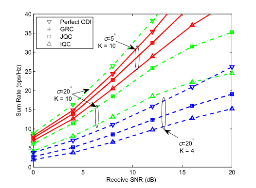
Figure 2: Average sum rates of 3D MIMO systems using URA for different angular spreads and numbers of users, where $N_{h}=N_{v}=8$ and $B=8$.

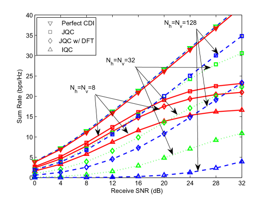
Figure 3: Average sum rates of 3D MIMO systems using URA with different sizes, where $K=4$, $\sigma=20^{\circ}$, and $B=8$.

The average sum rates of 3D MIMO systems using the URAs with different sizes are shown in Fig. 3. To show the impact of imperfect statistical information, we also evaluate the performance of the joint CDI quantization codebook with quantized statistical information (labeled as “JQ w/DFT”). The statistical sub-direction information in horizontal and vertical directions are respectively quantized by a 8-bit DFT codebook [20], where each codeword consists of $r_{h}$ and $r_{v}$ adjacent columns in the DFT matrix. The values of $r_{h}$ and $r_{v}$ are selected to quantize the first $r_{h}$ and $r_{v}$ dominant directions such that $\frac{\sum_{i=1}^{r_{h}}{{\lambda}_{h,i}}}{\sum_{i=1}^{N_{h}}{{\lambda}_{h,i}}}>0.9$ and $\frac{\sum_{i=1}^{r_{v}}{{\lambda}_{v,i}}}{\sum_{i=1}^{N_{v}}{{\lambda}_{v,i}}}>0.9$, where ${\lambda}_{h,i}$ and ${\lambda}_{v,i}$ are the $i$th element in $\boldsymbol{\lambda}_{h}$ and $\boldsymbol{\lambda}_{v}$ respectively. The power coupling matrix are quantized by a 8-bit RVQ codebook.

As shown in the figure, when the array size increases, the performance gaps of the joint CDI quantization codebooks with perfect and quantized statistical information keep almost constant under different SNRs and numbers of antennas. This is because the DFT codewords is a natural choice for representing the statistical directions for 3D MIMO with URA, as shown in [11]. Moreover, when the array size increases, the performance gap between the joint and independent CDI quantization codebook increases. This is because the rank of channel matrix increases with the size of antenna array even for a fixed angular spread. It is seen in the figure, as the size of antenna array increases, the sum rate gap between perfect CDI and the globally rotated codebook are reduced. This is because the inter-user interferences are reduced in the large antenna array when the full spatial correlation information is available. It indicates the importance of exploiting the channel correlation information in the codebook design in large array systems.

VI-A2 Performance for 3D MIMO Systems with UCCA

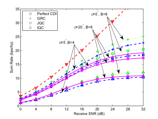
Figure 4: Average sum rates of 3D MIMO systems using UCCAs with different angle spread and number of bits, where $K=4$ and $\sigma=5^{\circ}$.

We then evaluate the performance of joint CDI quantization codebook for 3D MIMO systems using the UCCA at the BS. The configuration of UCCA is given by $J=8$, $L=8$, $d_{1}=0.5\lambda$, and $d_{j}=d_{j-1}+0.5\lambda$ for $1<j\leq J$. The average sum rates of 3D MIMO systems are shown in Fig. 4. When obtaining the statistical information by using the proposed explicit solution, we set the dimensionality as $N_{h}=N_{v}=8$, and similar results can be observed by other settings.

As shown in the figure, under different angular spreads and numbers of bits, the performance of joint CDI quantization codebook is inferior to that of rotated codebook but with acceptable performance loss. Moreover, the joint CDI quantization outperforms the independent quantization significantly.

VI-B Results in More Realistic Scenarios

In this subsection, we consider more realistic scenarios in the simulations. The azimuth and elevation angles in the channel are modeled by log-normal distributions as in [29], where two scenarios are evaluated: 3D urban micro (UMi) with non line-of-sight (NLOS), which is referred as 3D UMi, and 3D urban macro (UMa) with NLOS from an outdoor BS to an indoor user, which is referred as 3D UMa. The antenna spacing is $0.5\lambda$ for both horizontal and vertical directions. Unless otherwise specified, the main 3D MIMO channel parameters are listed in Table I, where $d$ is the distance from the BS to the user, $h$ is the height of each user. We set $d=100$ m for 3D UMi, and $d=250$ m, $h=1.5$ m for 3D UMa. This channel modeling considers more practical issues, such as the distance-dependent channel statistics, and the coupling effect between the statistics like delay spread and angular spread, which is more complicated than the simplified one in the previous subsection.

TABLE I: Main Parameters of 3D MIMO Channels

Scenario	3D UMi	3D UMa
Mean of azimuth clusters	$\boldsymbol{U}(-60^{\circ},~{}60^{\circ})$	$\boldsymbol{U}(-60^{\circ},~{}60^{\circ})$
Mean of elevation clusters	$\boldsymbol{U}(-45^{\circ},~{}45^{\circ})$	$\boldsymbol{U}(-45^{\circ},~{}45^{\circ})$
Mean of log delay spread (DS) ($\log_{10}([s])$)	-6.89	-6.62
Variance of log DS ($\log_{10}([s])$)	0.54	0.32
Mean of log azimuth spread (AS) ($\log_{10}([^{\circ}])$)	1.41	1.25
Variance of log AS ($\log_{10}([^{\circ}])$)	0.17	0.42
Mean of log elevation spread (ES) ($\log_{10}([^{\circ}])$)	$\max[-0.5,-2.1(d/1000)+0.9]$	$\max[-0.5,-2.1(d/1000)-0.01(h-1.5)+0.9]$
Variance of log ES ($\log_{10}([^{\circ}])$)	0.6	0.49
Number of clusters	19	12
Number of rays per cluster	20	20

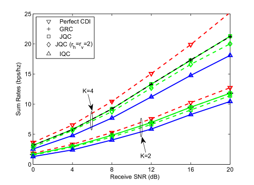
(a) 3D UMi

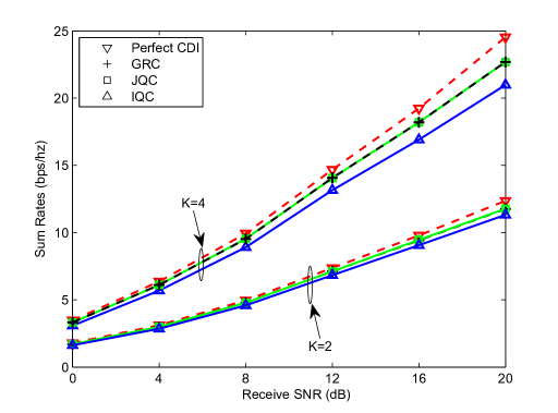
(b) 3D UMa

Figure 5: Average sum rates of $8\times 8$ 3D MIMO systems with $B=4$.

We evaluate the average sum rate of an $8\times 8$ 3D MIMO system using the joint CDI quantization codebook with different codeword dimension: JQC with full dimension ($r_{h}=N_{h}$ and $r_{v}=N_{v}$); JQC with low dimension ($r_{h}=2$ and $r_{v}=2$).

The average sum rates of the 3D MIMO systems with the URA are shown in Fig. 5, where 3D UMi and 3D UMa channels are respectively used. It is shown that the joint CDI quantization codebook with full dimension achieves the same performance as the globally rotated codebook. Even when using the joint CDI quantization codebook with reduced quantization dimension, there is still substantial performance gain over the independent CDI quantization codebook. In both scenarios, when the number of users $K$ grows, the performance gap between the joint and independent CDI quantization increases. The results are similar to the ones obtained in previous subsection.

Compared with 3D UMa, the performance gap between the joint and independent CDI quantization is larger in 3D UMi under the same number of users. This is because the scattering environment in 3D UMi is richer than in 3D UMa due to large variance given by the parameters of log-normal distribution.

VII Conclusions

We proposed a joint CDI quantization codebook for 3D MIMO systems in this paper. By exploiting the unique features of 3D MIMO channels, the proposed codebook is composed of codewords with a special structure, reflecting different types of information in the 3D MIMO channel direction. The proposed codebook is easily adapted to different spatially correlated channels and is applicable to different forms of arrays. Analytical analysis indicated that the proposed codebook achieves the same performance as the globally rotated codebook for uniform rectangular array under very general channel conditions but needs much less spatial correlation information. Simulation results validated the analysis and shown substantial performance gain over independent CDI quantization.

Appendix A Proof of Lemma 1

For notational simplicity, we express the $i$th column of 3D MIMO channel matrix $\boldsymbol{H}$ in (1) and the $j$th column of its transpose $\boldsymbol{H}^{T}$ as,

$$\boldsymbol{c}_{i} =\sum\nolimits_{n=1}^{N}\sum\nolimits_{m=1}^{M}g_{n,m}a_{v,i}(\phi_{n,m})\boldsymbol{a}_{h}(\theta_{n,m})$$

$$\boldsymbol{r}_{j} =\sum\nolimits_{n=1}^{N}\sum\nolimits_{m=1}^{M}g_{n,m}a_{h,j}(\theta_{n,m})\boldsymbol{a}_{v}(\phi_{n,m})$$ (29)

where $a_{v,i}(\phi_{n,m})$ and $a_{h,j}(\theta_{n,m})$ are respectively the $i$th entry of vector $\boldsymbol{a}_{v}(\phi_{n,m})$ and the $j$th entry of $\boldsymbol{a}_{h}(\theta_{n,m})$, $1\leq i\leq N_{h}$, $1\leq j\leq N_{v}$.

We can set $\acute{\boldsymbol{H}}=\boldsymbol{U}_{h}\boldsymbol{H}_{t}$, where $\boldsymbol{U}_{h}$ and $\boldsymbol{H}_{t}$ are defined in Proposition 1.

Denote the $i$th column of $\acute{\boldsymbol{H}}$ as $\acute{\boldsymbol{c}}_{i}$, the $k$th row of $\acute{\boldsymbol{H}}$ as $\acute{\boldsymbol{r}}_{k}^{T}$, and the $\ell$th entry of $\acute{\boldsymbol{r}}_{k}$ as $\acute{\boldsymbol{r}}_{k,\ell}$. Then, we have

$$\acute{\boldsymbol{r}}_{k}=\boldsymbol{U}_{v}^{H}\boldsymbol{r}_{k}$$ (30)

The cross-correlation matrix between the $i$th and $j$th column of $\acute{\boldsymbol{H}}$ for $i\neq j$ can be obtained as

$$\boldsymbol{E}\{\acute{\boldsymbol{c}}_{i}\acute{\boldsymbol{c}}_{j}^{H}\}=\boldsymbol{E}\left\{[\acute{\boldsymbol{r}}_{1,i}\cdots\acute{\boldsymbol{r}}_{N_{h},i}]^{T}[\acute{\boldsymbol{r}}^{\ast}_{1,j}\cdots\acute{\boldsymbol{r}}^{\ast}_{N_{h},j}]\right\}$$ (31)

For a 3D MIMO system with URA, for any $1\leq k,\ell\leq N_{v}$ and $k\neq\ell$, by using (29) we have

$$E\{\boldsymbol{r}_{k}\boldsymbol{r}_{\ell}^{H}\}\! =\!E\Big{\{}\big{(}\sum_{n=1}^{N}\sum_{m=1}^{M}g_{n,m}a_{h,k}(\theta_{n,m})\boldsymbol{a}_{v}(\phi_{n,m})\big{)}$$

$$\quad\quad\big{(}\sum_{n=1}^{N}\sum_{m=1}^{M}g_{n,m}a^{\ast}_{h,\ell}(\theta_{n,m})\boldsymbol{a}^{H}_{v}(\phi_{n,m})\big{)}\Big{\}}$$

$$\!=\!\sum_{n=1}^{N}\!\sum_{m=1}^{M}\!\!E\{|g_{n,m}|^{2}\}E\{a_{h,k}(\theta_{n,m})a^{\ast}_{h,\ell}(\theta_{n,m})$$

$$\quad\quad\boldsymbol{a}_{v}(\phi_{n,m})\boldsymbol{a}^{H}_{v}(\phi_{n,m})\}$$ (32)

$$\!=\!\sum_{n=1}^{N}\!\sum_{m=1}^{M}\!\!E\{|g_{n,m}|^{2}\}E\{a_{h,k}(\theta_{n,m})a^{\ast}_{h,\ell}(\theta_{n,m})\}\cdot$$

$$\quad\quad\boldsymbol{E}\{\boldsymbol{a}_{v}(\phi_{n,m})\boldsymbol{a}^{H}_{v}(\phi_{n,m})\}$$ (33)

which are derived under the assumption of weak i.i.d. rays: (32) is because the gains $g_{n,m}$ are uncorrelated with each other and also independent with the angles $\theta_{n,m}$ and $\phi_{n,m}$; and (33) is because the angle $\theta_{n,m}$ is independent with $\phi_{n,m}$.

For i.i.d. variables $\phi_{n,m}$, we have

$$\boldsymbol{E}\{\boldsymbol{a}_{v}(\phi_{n,m})\boldsymbol{a}^{H}_{v}(\phi_{n,m})\}\triangleq\boldsymbol{R}_{v}^{0}=\boldsymbol{U}_{v}\boldsymbol{\Lambda}_{v}^{0}\boldsymbol{U}_{v}^{H},~{}\text{for}~{}\forall n~{}\text{and}~{}m$$ (34)

where the last equality is the SVD decomposition of positive semi-definite Hermitian correlation matrix $\boldsymbol{R}_{v}^{0}$, and $\boldsymbol{\Lambda}_{v}^{0}$ is a positive diagonal matrix.

Then, from (33) and (34), we have

$$E\{\boldsymbol{r}_{k}\boldsymbol{r}_{\ell}^{H}\} =\boldsymbol{U}_{v}\boldsymbol{\Lambda}_{v}^{k\ell}\boldsymbol{U}_{v}^{H}$$ (35)

where

$$\boldsymbol{\Lambda}_{v}^{k\ell}=\boldsymbol{\Lambda}_{v}^{0}\sum\limits_{n=1}^{N}\!\sum\limits_{m=1}^{M}\!E\{|g_{n,m}|^{2}\}E\{a_{h,k}(\theta_{n,m})a^{\ast}_{h,\ell}(\theta_{n,m})\}$$

is diagonal.

From (30) and (35), we have

$$\boldsymbol{E}\{\acute{\boldsymbol{r}}_{k}\acute{\boldsymbol{r}}_{\ell}^{H}\}=\boldsymbol{U}_{v}^{H}\boldsymbol{E}\{\boldsymbol{r}_{k}\boldsymbol{r}^{H}_{\ell}\}\boldsymbol{U}_{v}=\boldsymbol{\Lambda}_{v}^{k\ell}$$ (36)

and

$$\boldsymbol{E}\{\acute{r}_{k,i}\acute{r}_{\ell,j}^{H}\}=0,~{}\forall k\neq\ell\text{~{}and~{}}i\neq j,$$ (37)

because the off-diagonal elements of matrix $\boldsymbol{\Lambda}_{v}^{k\ell}$ are zero.

From (31) and (37), we obtain

$$\boldsymbol{E}\{\acute{\boldsymbol{c}}_{i}\acute{\boldsymbol{c}}_{j}^{H}\}=\boldsymbol{0},\forall i\neq j$$ (38)

which means that the columns of $\acute{\boldsymbol{H}}$ are uncorrelated with each other. The lemma is proved.

Appendix B Proof of Lemma 3

Denote the $n$th column of $\boldsymbol{H}_{t}$ as $\boldsymbol{c}_{tn}$. By letting $\boldsymbol{H}_{t}=\boldsymbol{U}_{h}^{H}\acute{\boldsymbol{H}}$, i.e., $\boldsymbol{c}_{tn}=\boldsymbol{U}_{h}^{H}\acute{\boldsymbol{c}}_{n}$, for $n\neq m$ we find that

$$\boldsymbol{E}\{\boldsymbol{c}_{tn}\boldsymbol{c}_{tm}^{H}\}=\boldsymbol{U}_{h}^{H}\boldsymbol{E}\{\acute{\boldsymbol{c}}_{n}\acute{\boldsymbol{c}}^{H}_{m}\}\boldsymbol{U}_{h}=\boldsymbol{0},\forall n\neq m$$ (39)

where the last equality is from (38) in Lemma 1.

Similarly, denote the $n$th row of $\boldsymbol{H}_{t}$ as $\boldsymbol{r}_{tn}^{T}$. By letting $\boldsymbol{H}_{t}=\grave{\boldsymbol{H}}\boldsymbol{U}_{v}^{\ast}$, i.e., $\boldsymbol{r}_{tn}=\boldsymbol{U}_{v}^{H}\grave{\boldsymbol{r}}_{n}$, for $n\neq m$ we find that

$$\boldsymbol{E}\{\boldsymbol{r}_{tn}\boldsymbol{r}_{tm}^{H}\}=\boldsymbol{U}_{v}^{H}\boldsymbol{E}\{\grave{\boldsymbol{r}}_{n}\grave{\boldsymbol{r}}^{H}_{m}\}\boldsymbol{U}_{v}=\boldsymbol{0},\forall n\neq m$$ (40)

where the last equality is obtained from Lemma 2.

From (39) and (40), the entries in $\boldsymbol{H}_{t}$ are uncorrelated. The lemma is proved.

Appendix C Proof of Theorem

From Lemma 3, the entries of $\boldsymbol{H}_{t}$ are uncorrelated. When the spatial correlation matrix of the 3D MIMO channels is perfect, from (13) we have

$$\boldsymbol{\hat{R}}=\boldsymbol{R} =\boldsymbol{E}\{\text{vec}(\boldsymbol{H})\text{vec}(\boldsymbol{H})^{H}\}$$

$$=(\boldsymbol{U}_{v}\otimes\boldsymbol{U}_{h})\text{diag}(\text{vec}\{\boldsymbol{\Lambda}\odot{\boldsymbol{\Lambda}}\})(\boldsymbol{U}_{v}\otimes\boldsymbol{U}_{h})^{H}$$

Then, the rotation matrix used in the globally rotated codeword in (6) is

$$\boldsymbol{R}^{1/2}=(\boldsymbol{U}_{v}\otimes\boldsymbol{U}_{h})\text{diag}(\text{vec}\{\boldsymbol{\Lambda}\})$$ (41)

which is the same as the rotation matrix used in the joint CDI quantization (11) when the statistical information $\hat{\boldsymbol{U}}_{h}=\boldsymbol{U}_{h}$, $\hat{\boldsymbol{U}}_{v}={\boldsymbol{U}}_{v}$, and $\hat{\lambda}=\text{vec}({\boldsymbol{\Lambda}})$ are perfect.

Therefore, when all the instantaneous codewords for the joint CDI quantization codebook and those for the globally rotated codebook are identical, the two codebooks achieve the same performance. The theorem is proved.

References

- [1] E. G. Larsson, O. Edfors, and T. L. Marzetta, “Massive MIMO for Next Generation Wireless Systems,” IEEE Commun. Mag., vol. 52, no. 2, pp. 186–195, Feb. 2014.
- [2] Y.-H. Nam, B. L. Ng, K. Sayana, Y. Li, J. Zhang, Y. Kim, and J. Lee, “Full-dimension MIMO (FD-MIMO) for next generation cellular technology,” IEEE Commu. Mag., pp. 172–179, Jun. 2013.
- [3] “Requirements, candidate solutions and technology roadmap for LTE Rel-12 onward,” NTT docomo, 3GPP Workshop on Release 12 and onwards, RWS120010, 2012.
- [4] “Considerations on CSI feedback enhancements for high-priority antenna configurations,” Alcatel-Lucent Shanghai Bell, 3GPP TSG-RAN WG1 66,R1-112420, 2011.
- [5] W. Roh, J. Seol, J. Park, B. Lee, J. Lee, Y. Kim, J. Cho, K. Cheun, and F. Aryanfar, “Millimeter-wave beamforming as an enabling technology for 5G cellular communications: Theoretical feasibility and prototype results,” IEEE Communi. Magazine, vol. 52, no. 2, pp. 106–113, Feb. 2014.
- [6] J. Jose, A. Ashikhmin, T. L. Marzetta, and S. Vishwanath, “Pilot contamination and precoding in multi-cell TDD systems,” IEEE Trans. Wireless Commun., vol. 10, no. 8, pp. 2640–2651, Aug. 2011.
- [7] D. J. Love, R. W. Heath Jr., and T. Strohmer, “Grassmannian beamforming for multiple-input multiple-output wireless systems,” in Proc. IEEE Int. Communi. Conf., 2003.
- [8] N. Jindal, “MIMO broadcast channels with finite-rate feedback,” IEEE Trans. Inform. Theory, vol. 52, no. 11, pp. 5045–5060, Nov. 2006.
- [9] “WINNER+ final channel models,” D5.3 v1.0.
- [10] B. Clerckx, G. Kim, and S. Kim, “Correlated fading in broadcast MIMO channels: Curse or blessing?” in Proc. IEEE Global Telecommun. Conf., 2008.
- [11] A. Adhikary, J. Nam, J.-Y. Ahn, and G. Caire, “Joint spatial division and multiplexing the large-scale array regime,” IEEE Trans. Inform. Theory, vol. 59, no. 10, pp. 6441–6463, Oct. 2013.
- [12] P.-H. Kuo, H. Kung, and P.-A. Ting, “Compressive sensing based channel feedback protocols for spatially-correlated massive antenna arrays,” in IEEE Wireless Communi. and Netw. Conf., 2012.
- [13] J. Choi, D. Love, and P. Bidigare, “Downlink training techniques for FDD massive MIMO systems: Open-loop and closed-loop training with memory,” IEEE J. Select. Sig. Process., vol. 8, no. 5, pp. 802–814, Oct. 2014.
- [14] A. Gersho and R. M. Gray, Vector Quantization and Signal Compression. Kluwer, 1992.
- [15] V. Raghavan, R. W. Heath Jr., and A. M. Sayeed, “Systematic codebook designs for quantized beamforming in correlated MIMO channels,” IEEE J. Select. Areas Commun., vol. 25, no. 7, pp. 1298–1310, Sep. 2007.
- [16] Y. Huang, L. Yang, M. Bengtsson, and B. Ottersten, “Exploiting long-term channel correlation in limited feedback SDMA through channel phase codebook,” IEEE Trans. Signal Processing, vol. 59, no. 3, pp. 1217–1228, Mar. 2011.
- [17] D. J. Love and R. W. Heath Jr., “Limited feedback diversity techniques for correlated channels,” IEEE Trans. Veh. Technol., vol. 55, no. 2, pp. 718–722, Feb. 2006.
- [18] J. Zheng and B. D. Rao, “Analysis of multiple antenna systems with finite-rate channel information feedback over spatially correlated fading channels,” IEEE Trans. Signal Processing, vol. 55, no. 9, pp. 4612–4626, Sep. 2007.
- [19] J. Choi, V. Raghavan, and D. J. Love, “Limited feedback design for the spatially correlated multi-antenna broadcast channel,” in IEEE Global Telecommuni. Conf., 2013.
- [20] D. Yang, L.-L. Yang, and L. Hanzo, “DFT-based beamforming weight-vector codebook design for spatially correlated channels in the unitary precoding aided multiuser downlink,” in Proc. IEEE Int. Communi. Conf., 2010.
- [21] Y. Xie, S. Jin, J. Wang, Y. Zhu, X. Gao, and Y. Huang, “A limited feedback scheme for 3D multiuser MIMO based on kronecker product codebook,” in Proc. IEEE Pers. Indoor and Mob. Radio Communi., 2013.
- [22] J. Choi, B. Clerckx, N. Lee, and G. Kim, “A new design of polar-cap differential codebook for temporally/spatially correlated MISO channels,” IEEE Trans. Wireless Commun., vol. 11, no. 2, pp. 703–711, Feb. 2012.
- [23] R. Marimont and M. Shapiro, “Nearest neighbour searches and the curse of dimensionality,” IMA J. of Applied Mathematics, vol. 24, no. 1, pp. 59–70, 1978.
- [24] T. Marzetta, G. Tucci, and S. Simon, “A random matrix-theoretic approach to handling singular covariance estimates,” IEEE Trans. Inform. Theory, vol. 57, no. 9, pp. 6256–6271, Sep. 2011.
- [25] S. Ragnarsson, “Structured tensor computations: Blocking, symmetries and kronecker factorizations,” Ph.D. dissertation, Cornell Univ., 2012.
- [26] J.-Y. Ko and Y.-H. Lee, “Adaptive beamforming with dimension reduction in spatially correlated MISO channels,” IEEE Trans. Wireless Commun., vol. 8, no. 10, pp. 4998–5002, Oct. 2009.
- [27] S. Rajagopal, S. Abu-Surra, Z. Pi, and F. Khan, “Antenna array design for multi-Gbps mmwave mobile broadband communication,” in Proc. IEEE Global Telecommuni. Conf., 2011.
- [28] S. K. Yong and J. S. Thompson, “A three-dimensional spatial fading correlation model for uniform rectangular arrays,” IEEE Ant. and Wireless Propa. letters, vol. 2, pp. 182–185, 2003.
- [29] “3rd Generation Partnership Project; technical specification group radio access network; study on 3D channel model for LTE (release 12),” 3GPP TR36.873, V1.2.0, 2013.
- [30] H. L. V. Trees, Optimum Array Processing, Part IV of Detection, Estimation and Modulation Theory. Wiley, 2002.
- [31] J. Choi, Z. Chance, D. Love, and U. Madhow, “Noncoherent trellis coded quantization: A practical limited feedback technique for massive MIMO systems,” IEEE Trans. Commun., vol. 61, no. 12, pp. 5016–5029, Dec. 2013.
- [32] B. Hochwald and T. Maretta, “Adapting a downlink array from uplink measurements,” IEEE Trans. Signal Processing, vol. 49, no. 3, pp. 642–653, Mar 2001.
- [33] S. Ghosh, B. Rao, and J. Zeidler, “Techniques for MIMO channel covariance matrix quantization,” IEEE Trans. Signal Processing, vol. 60, no. 6, pp. 3340–3345, Jun. 2012.
- [34] R. Krishnamachari, M. Varanasi, and K. Mohanty, “MIMO systems with quantized covariance feedback,” IEEE Trans. Signal Processing, vol. 62, no. 2, pp. 485–495, Jan 2014.
- [35] N. P. Pitsianis, “The kronecker product in approximation and fast transform generation,” Ph.D. dissertation, Cornell Univ., 1997.
- [36] A. Wiesel, Y. Eldar, and S. Shamai, “Zero-forcing precoding and generalized inverses,” IEEE Trans. Signal Processing, vol. 55, no. 9, pp. 4409–4418, Sep. 2008.
- [37] N. Ravindran, N. Jindal, and H. C. Huang, “Beamforming with finite rate feedback for LOS MIMO downlink channels,” in Proc. IEEE Global Telecommun. Conf., 2007.