Photoionization Heating of Nova Ejecta by the Post-Outburst Supersoft Source

Abstract

The expanding ejecta from a classical nova remains hot enough ($\sim 10^{4}\,{\rm K}$) to be detected in thermal radio emission for up to years after the cessation of mass loss triggered by a thermonuclear instability on the underlying white dwarf (WD). Nebular spectroscopy of nova remnants confirms the hot temperatures observed in radio observations. During this same period, the unstable thermonuclear burning transitions to a prolonged period of stable burning of the remnant hydrogen-rich envelope, causing the WD to become, temporarily, a super-soft X-ray source. We show that photoionization heating of the expanding ejecta by the hot WD maintains the observed nearly constant temperature of $(1-4)\times 10^{4}\mathrm{~{}K}$ for up to a year before an eventual decline in temperature due to either the cessation of the supersoft phase or the onset of a predominantly adiabatic expansion. We simulate the expanding ejecta using a one-zone model as well as the Cloudy spectral synthesis code, both incorporating the time-dependent WD effective temperatures for a range of masses from $0.60\ M_{\odot}$ to $1.10\ M_{\odot}$. We show that the duration of the nearly isothermal phase depends most strongly on the velocity and mass of the ejecta and that the ejecta temperature depends on the WD’s effective temperature, and hence its mass.

1. Introduction

Classical novae (CNe) are caused by the ejection of $\Delta M_{\rm ej}\sim 10^{-4}\,M_{\odot}$ of matter from an accreting white dwarf (WD) triggered by a thermonuclear instability in recently-accreted hydrogen-rich matter (Gallagher & Starrfield, 1978; Starrfield et al., 2008). The expanding ejecta are bright in the radio for hundreds of days after the optical peak (Seaquist & Bode, 2008) and are well modeled by assuming the radiation comes from thermal bremsstrahlung emission from an expanding medium of nearly constant electron temperature $T_{e}\approx(1-4)\times 10^{4}$ K (Seaquist & Palimaka, 1977; Hjellming et al., 1979; Taylor et al., 1988; Eyres et al., 1996). Such temperatures are also observed via nebular spectroscopy long after optical peak in novae like V1974 Cygni 1992 (Austin et al., 1996) and T Pyxidis V351 (Shore et al., 2013). However, between the fading of the optical emission (which may correspond to the end of mass ejection) and the end of the radio emission several hundred days later, the ejecta undergo an expansion in volume by several orders of magnitude. In the absence of a heating source, the ejecta would undergo adiabatic expansion, leading to a large temperature decline to values orders of magnitude less than the observed $10^{4}$ K. The cause of these much higher temperatures for such prolonged periods is the focus of this paper.

With the rise of frequent X-ray monitoring of classical novae, it is becoming increasingly clear that most, if not all, CNe are followed by a super-soft X-ray source (SSS) phase during which the WD shrinks in radius to nearly its pre-nova size, but continues to burn a remnant hydrogen envelope at nearly the Eddington luminosity as modeled by Starrfield et al. (1974), Fujimoto (1982), Sala & Hernanz (2005), Hachisu & Kato (2010), and Wolf et al. (2013). This phase has been decteced in many galactic novae (Oegelman et al., 1984; Shore, 2008; Krautter, 2008; Schwarz et al., 2011), and observations in M31 are making it clear that a SSS phase is likely to follow every classical nova outburst (Henze et al., 2011, 2014b). During the SSS phase, the WD has $L\approx 10^{4}\,L_{\odot}$ and since it is compact, is a strong source of radiation at $kT_{\mathrm{eff}}\approx 50-100$ eV. This SSS phase can be as short as a few days for novae with the most massive WDs (Tang et al., 2014; Henze et al., 2014a) and as long as a decade for low-mass WDs like V723 Cas (Ness et al., 2008). We show here that the SSS phase is a sufficiently powerful source of photoionizing heating to sustain the high ejecta temperature long after the optical peak.

We start in Section 2 by reviewing the physics of photoionization balance and establish our simplified model of hydrogen and helium ionization in nova ejecta. We derive the temporal evolution of the ejecta temperature in Section 3 and discuss computational models in Section 4. We compare our semi-analytic results to the computational results in Section 5, and end by showing how this new understanding can inform us about the properties of CNe ejecta, and, potentially, the WD mass.

2. Photoionization Balance

For the late time evolution of interest to us, we chose to model the nova ejecta at age $t$ as one zone of constant mass $\Delta M_{\mathrm{ej}}$ in a uniform density sphere (i.e. not a shell) of radius $r(t)=v_{\mathrm{ej}}t$ expanding at constant velocity $v_{\mathrm{ej}}$. A hot WD of mass $M$ and radius $R_{\mathrm{WD}}$ resides at the center. The ejecta has a composition $\mathbf{X}$, here represented as a vector of mass fractions. The number density of any given isotope, $i$, in the ejecta is

$$n(X_{i})=\frac{3X_{i}\Delta M_{\mathrm{ej}}}{A_{i}m_{p}4\pi v_{\mathrm{ej}}^{3}t^{3}},$$ (1)

where $A_{i}$ is the mass number of isotope $i$ and $m_{p}$ is the proton mass. The electron-ion coupling time is always much shorter than the age, $t$, during the time relevant for our calculations, so there is only one temperature, $T(t)$. We express the fundamental equation of thermodynamics in terms of ejecta volume $V$, entropy $S$, and total number of particles $N$ as

$$TdS =NkT\left(\frac{3dT}{2T}+\frac{dV}{V}\right)\ .$$ (2)

For a spherical ejecta of pure ionized hydrogen ($N=2N_{e}$) with $r=vt$, this becomes

$$T\frac{ds}{dt} =n_{e}kT\left(3\frac{d}{dt}\ln T+\frac{6}{t}\right)\ .$$ (3)

where we now consider the specific entropy $s=S/V$ and $n_{e}$ is the number density of electrons.

The only source of heating we will consider is that from the central, hot, WD in the SSS phase, which is a system that has been modeled extensively (Starrfield et al., 1974; Fujimoto, 1982; MacDonald & Vennes, 1991; Sala & Hernanz, 2005; Hachisu & Kato, 2010; Wolf et al., 2013). We extended the work of Wolf et al. (2013) to generate the time-dependence of $T_{\rm eff}$ for a range of WD masses, as shown in Figure 1. These simulations used the 1-D stellar evolution code MESA (Paxton et al., 2011, 2013), following the time-dependent evolution of WDs accreting solar composition material at $10^{-9}\ M_{\odot}\ \mathrm{yr^{-1}}$ through several nova flashes with super-Eddington winds as the primary mode of mass loss. In particular, we only display the results from the end of mass loss until the end of quasi-stable hydrogen burning for one representative nova cycle. The original simulations did not have data for a 0.8 or 1.1 $M_{\odot}$ WD, so we generated additional data for this work. At any given age since mass loss ended, we know the WD radius and $T_{\rm eff}$, and hence the radiation field that powers the photoionization heating. This is the only information we use from the MESA models. The ejecta parameters $\Delta M_{\mathrm{ej}}$ and $v_{\mathrm{ej}}$ used are independent of the MESA models, and, in general, would vary significantly for novae on WDs of different masses.

2.1. Strömgren Breakout

Our first concern is whether the photoionization source is adequate to maintain a large region of mostly ionized plasma in the ejecta. Hence, we start by finding the Strömgren sphere radius, $R_{\mathrm{S}}$, and compare it to the ejecta dimension, $v_{\mathrm{ej}}t$. For simplicity, we assume pure ionized hydrogen ($n_{e}=n_{p}$) within the Strömgren sphere, and equate the rate of emission of H-ionizing photons by the WD, $Q_{\rm H}$, with the rate of recombinations in that volume,

$$Q_{\rm H}=\frac{4}{3}\pi R_{\rm S}^{3}\alpha n_{\rm p}n_{e}\ ,$$ (4)

where $\alpha$ is the radiative recombination rate of hydrogen.

At early times $R_{\rm S}$ is far inside the outer ejecta radius, $v_{\mathrm{ej}}t$, and the ratio scales as

$$\frac{R_{\rm S}}{v_{\mathrm{ej}}t}=\left(\frac{4\pi Q_{\rm H}}{3\alpha N_{p}^{2}}\right)^{1/3}(v_{\mathrm{ej}}t),$$ (5)

where $N_{p}$ is the total number of protons. Hence, at early times, the Strömgren sphere is inside the ejecta, and only breaks out at an age of

$$\small t_{\rm S}\approx 30~{}\mathrm{d}\left(\frac{v_{\mathrm{ej}}}{10^{3}~{}\mathrm{km/s}}\right)^{-1}\left(\frac{\Delta M_{\mathrm{ej}}}{10^{-5}~{}M_{\odot}}\right)^{2/3}\left(\frac{Q_{\rm H}}{10^{48}~{}\mathrm{s}^{-1}}\right)^{-1/3}\ .$$ (6)

where we have scaled $v_{\mathrm{ej}}$, $\Delta M_{\mathrm{ej}}$, and $Q_{\mathrm{H}}$ to values typical of novae on intermediate-mass WDs. Table 1 shows that the H Strömgren sphere breaks out by 50 days for all but the most massive WDs for $\Delta M_{\mathrm{ej}}=10^{-5}\ M_{\odot}$ and $v_{\mathrm{ej}}=10^{3}\ \mathrm{km\,s^{-1}}$. This confirms a time after which all of the ejecta is exposed to the photoionizing radiation field. The pure He breakout times for singly ionized He Strömgren spheres are systematically later due to less ionizing radiation available for a pure He ejecta. The more massive WDs have longer Strömgren breakout times at the same ejecta parameters because while they produce harder spectra than lower-mass models, the total luminosity is not significantly higher, so the total number of ionizing photons emitted, $Q$, decreases, requiring more time for a complete ionization of the ejecta. Additionally, the SSS phases for the most massive models are short enough that the ionization front never makes it to the ejecta radius before the ionizing source fades greatly, causing excessively long Strömgren breakout times. We explore the ionization state of the ejecta at late times in Section 5.

Beck et al. (1990) performed a much more detailed calculation of this breakout for a He Strömgren sphere for a mixed ejecta with heavier elements ($Z>2$), and a lower ejected mass and velocity ($\Delta M_{\mathrm{ej}}=1.3\times 10^{-6}~{}M_{\odot}$ and $v_{\rm ej}=6\times 10^{2}\mathrm{~{}km~{}s^{-1}}$ than we used for Table 1. So as to make a close comparison, we used their parameters, including their WD $T_{\rm eff}$ (see Figure 6 of Beck et al., 1990) as inputs to our homogenous model. We found that the H and He Strömgren breakouts occur at 31 days and 77 days, respectively, very close to the breakout they reported at $t=76\mathrm{~{}d}$ for the He Strömgren sphere.

Table 1Strömgren Breakout Times

		H			He
$M_{\mathrm{WD}}$		$t_{\mathrm{S}}$	$Q_{\mathrm{H},47}$		$t_{\mathrm{S}}$	$Q_{\mathrm{He},47}$
$(M_{\odot})$		(d)	$(10^{47}\ \mathrm{s^{-1}})$		(d)	$(10^{47}\ \mathrm{s^{-1}})$
0.60		31	8.0		95	1.2
0.80		28	11.0		69	3.6
1.00		31	8.0		60	5.6
1.10		37	5.0		67	4.4
1.20		41	4.0		214	3.6
1.30		132	2.9		387	2.7

2.2. Ionization Timescale

After the Strömgren breakout, we allow that the ejecta may no longer absorb the majority of the photoionizing radiation. We characterize this via the optical depth, $\tau_{\nu}$, through the ejecta at frequency $\nu$,

$$\tau_{\nu}(r)=\sum_{i}n(X_{i})~{}\sigma_{\rm pi}(\nu,X_{i})~{}r,$$ (7)

where $\sigma_{\rm pi}(\nu,X_{i})$ is the photoionization cross-section and the sum is over all isotopes in $\mathbf{X}$. The time an isotope can spend in the neutral state is set by the photoionization timescale, which we define at the ejecta outer radius ($r=v_{\mathrm{ej}}t$), giving

$$\frac{1}{t_{\rm ion}(X_{i})} =\pi\left(\frac{R_{\mathrm{WD}}}{r}\right)^{2}\int\limits_{I_{\rm X_{i}}/h}^{\infty}d\nu\,\frac{B_{\nu}(T_{\mathrm{eff}})}{h\nu}\sigma_{\rm pi}(\nu)\ ,$$ (8)

where $B_{\nu}(T_{\mathrm{eff}})$ is the Planck function evaluated for the WD $T_{\rm eff}$, and $I_{X_{i}}$ is the ionization energy for isotope $X_{i}$.

We consider only the two most significant elements for photoionization heating; H and He. We assume that after the breakout time $n(X_{i})$ is low enough that the ejecta is optically thin for Lyman limit photons ($h\nu=13.6\mathrm{~{}eV}$). In this limit we neglect any secondary ionization caused by a recombination emission (Baker & Menzel, 1938) and consider only hydrogenic ionization processes (essentially assuming there are no neutral helium atoms). This gives two dynamical expressions for the hydrogenic number density of hydrogen and helium, respectively

$$\dot{n}(H) =-\frac{n(\mathrm{H})}{t_{\mathrm{ion}}(\mathrm{H})}+n_{e}n(\mathrm{H}^{+})\alpha(T,\mathrm{H}^{+})\ ;$$ (9)

$$\dot{n}(\mathrm{He}^{+}) =-\frac{n(\mathrm{He}^{+})}{t_{\mathrm{ion}}(\mathrm{He}^{+})}+n_{e}n(\mathrm{He}^{++})\alpha(T,\mathrm{He}^{++})\ .$$ (10)

As long as the WD is emitting, we found that the timescale over which these quantities relax is orders of magnitude smaller than the age of the ejecta, so we can consider an instantaneous steady state solution, where $\dot{n}(X_{i})=0$, yielding

$$n(X_{i})\left(\frac{1}{t_{\rm ion}}+P_{\rm ci}(T,X_{i})\right)=n_{e}n(X_{i}^{+1})\alpha(T,X_{i}^{+1})\ ,$$ (11)

with $P_{\rm ci}(T,X_{i})$ the temperature-dependent collisional ionization rate which we adopt from Lang (1980). This equation yields the very small neutral fraction that we must know to calculate the heating rate from photoionization.

Figure 1.— The calculated time dependent $T_{\rm eff}$’s of different mass WDs as simulated by Wolf et al. (2013), including two new cases (0.80 & 1.10 $M_{\odot}$) here. The age is the time since the end of mass loss driven by the thermonuclear instability. The rapid decline at later times for the three most massive WDs corresponds to the end of their SSS phases.

3. Time-dependent Entropy Evolution

Now that we have shown that photoionization balance drives the neutral fraction to a low value after the breakout of the Strömgren sphere, we can consider the entropy evolution of the expanding ejecta, which will lead us to a temperature evolution. The photoionization heating timescale is much less than the age initially after breakout so that any information regarding the initial entropy is lost. This will simplify our calculation as we consider the state of the plasma under photoionization heating and radiative cooling, where we use a cooling function $\Lambda(T)$ determined by comparative simulations run in Cloudy as detailed in Section 4. The resulting rate of change of specific entropy $s$ is then

$$T\frac{ds}{dt}=\Gamma_{\rm pi}-\Lambda(T)\ ,$$ (12)

where the rate of photoionization heating, $\Gamma_{\rm pi}$, is given by

$$\Gamma_{\rm pi}=\sum\limits_{i}\frac{n(X_{i})}{t_{\rm ion}(X_{i})}E_{\rm ion}(X_{i})\ ,$$ (13)

with $E_{\rm ion}(X_{i})$ being the average photoelectron energy. Under the optically thin assumption $E_{\rm ion}$ is given by Draine (2011) as

$$E_{\rm ion}(X_{i})=\frac{\int\limits_{Z^{2}I_{\rm H}/h}^{\infty}d\nu\,\frac{B(\nu,T)}{h\nu}\sigma_{\rm pi}(\nu,X_{i})(h\nu-Z^{2}I_{\rm H})}{\int\limits_{Z^{2}I_{\rm H}/h}^{\infty}d\nu\,\frac{B(\nu,T)}{h\nu}\sigma_{\rm pi}(\nu,X_{i})}.$$ (14)

Using equations (3) and (12) we find the equation for $T(t)$ as

$$\frac{dT}{dt}=\frac{1}{3kn_{e}}\left[\Gamma_{\rm pi}-\Lambda(T)\right]-\frac{2T}{t}\ .$$ (15)

Finding a temperature evolution, $T(t)$, requires solving equations (13) & (15) simultaneously.

Before showing the detailed solutions of equation (15), it is best to first exhibit a few limits. The first limit is to assume that the plasma is nearly fully ionized, and that ionization balance is set by equation (11) but with little impact from collisional ionization. This yields a simple relation of $n_{\rm H}/t_{\rm ion}\approx n_{e}n_{p}\alpha$ and a heating rate of $\Gamma_{\rm pi}\approx E_{\rm ion}n_{e}n_{p}\alpha$. Since $t_{\rm ion}\ll t$ when the WD is hot, we found that ejecta of different initial temperatures would very rapidly (on a timescale much less than the age) reach a state of $\Gamma_{\rm pi}\approx\Lambda(T)$ and a temperature, $T_{\rm iso}$ nearly independent of the electron density. The scale of these heating and cooling terms (which nearly cancel in equation (15)) are so much larger than the $2T/t$ adiabatic expansion term that the ejecta evolves from one isothermal (heating balances cooling) state to the next under a condition of thermal and photoionization balance. The resulting nearly isothermal evolution of this phase then arises from the condition of $\Gamma_{\rm pi}\approx\Lambda(T)$ for different WD $T_{\rm eff}$’s. There is nearly no sensitivity to the actual electron density when in this limit, so ejecta clumping will not matter, and all initial entropy information is lost.

However, the heating term, $\Gamma_{\rm pi}/n_{e}$, in equation (15) is $\propto t^{-3}$, implying that there will come a time, which we call $t_{\rm iso}$, beyond which the heating term is comparable to, or less than, the adiabatic expansion term, $2T/t$, and we expect to see a temperature decline. If we neglect radiative cooling, this critical timescale, $t_{\rm iso}$, is when $\Gamma_{\rm pi}/3kn_{e}=E_{\rm ion}n_{p}\alpha/3k=2T/t$. For the case of pure, ionized Hydrogen this gives

$$t_{\rm iso}\approx 250\,\mathrm{d}\left(\frac{\Delta M_{\mathrm{ej}}}{10^{-5}~{}M_{\odot}}\right)^{1/2}\left(\frac{v_{\mathrm{ej}}}{10^{3}\mathrm{~{}km/s}}\right)^{-3/2}\\ \times\left(\frac{E_{\rm ion}}{10\mathrm{~{}eV}}\right)^{1/2}\left(\frac{kT}{1\mathrm{~{}eV}}\right)^{-1/2}\left(\frac{\alpha}{10^{-13}\ \mathrm{cm^{3}}\,\mathrm{s}^{-1}}\right)^{1/2}.$$ (16)

We will show in the following section that our detailed thermal evolution calculations for these remnants can be simply described by the arguments above, with nearly all solutions exhibiting a nearly isothermal phase for $t<t_{\rm iso}$, followed by a temperature decline.

4. Cloudy Simulations

We also simulated the nova ejecta using the radiative transfer code Cloudy (version 13.03, Ferland et al., 2013), which has been successfully used to model nova ejecta in the past by Schwarz (2002), Vanlandingham et al. (2005), and Schwarz et al. (2007). Cloudy allows a user to specify the density structure of a gas, its composition, and an incident radiation field. It then computes the ionization state of the material, yielding line strengths, temperatures, and many other details, including realistic cooling curves.

To make the models in Cloudy as similar to our semi-analytic approach as possible, we set the radiation field at a given time to be a blackbody spectrum with the $T_{\rm eff}$ and radius set by the MESA models for that WD mass. The constant density gas reaches an outer radius $r_{\mathrm{out}}(t)=v_{\mathrm{ej}}t$ and an inner radius $r_{\mathrm{in}}(t)=0.01r_{\mathrm{out}}(t)$ essentially reproducing our constant density sphere model. To account for temperature decline from adiabatic expansion, we insert a “cooling” term

$$\Lambda_{\mathrm{exp}}\approx 2\times 10^{-16}\Delta M_{\mathrm{ej},-5}\,v_{\mathrm{ej},3}^{-3}\,T_{4}\,t_{8}^{-4}\ \mathrm{erg\ s^{-1}\ cm^{-3}},$$ (17)

that matches the second term in equation (3), where $\Delta M_{\mathrm{ej},-5}=\Delta M_{\mathrm{ej}}/(10^{-5}\ M_{\odot})$, $v_{\mathrm{ej},3}=v_{\mathrm{ej}}/(1000\ \mathrm{km\ s^{-1}})$, $T_{4}=T/(10^{4}\ \mathrm{K})$, and $t_{8}=t/(10^{8}\ \mathrm{s})$. The ejecta material was set to have a solar (Cloudy’s default abundance set) composition so that cooling by metals would be included. We then divide the WD evolution histories into twenty-one times, divided equally in log age, and use Cloudy to compute a temperature/ionization structure for the ejecta. These calculations assume that the cloud has reached both a photoionization and thermal equilibrium with the applied radiation field. We already established in Section 3 that these are valid assumptions at early times while $t_{\mathrm{ion}}\ll t$, so these Cloudy simulations provide physically motivated snapshots at those early times of concern for us. Essentially, these simulations in their current form solve (15) assuming $dT/dt=0$ and do not incorporate dynamic effects other than the artificially inserted adiabatic cooling.

For these simulations, we found that the temperature was rather constant with radius, leading to a single temperature for each model that we defined as the mass-average over the outer 50% of the mass. These temperature histories are what we compare to the semi-analytic models in Section 5. For later use in our semi-analytic work (e.g. equation (15)) we also extracted a cooling curve by finding the volumetric cooling rate at each grid point, subtracting off the portion of that cooling due to expansion from equation (17), and then dividing by $n_{\mathrm{H}}n_{e}$. The resulting cooling curves depend on the WD $T_{\rm eff}$ (and hence WD mass) due to different degrees of ionization and line cooling. We thus generated characteristic Cloudy cooling curves for each WD mass by choosing a time in the Cloudy calculations about halfway through the observed temperature plateau in log age. At times beyond these, the heating and cooling timescales become comparable to the age, and we can no longer trust the equilibrium Cloudy calculation, but rather should solve the fully time-dependent problem. We make progress on that aspect in the Section 5.

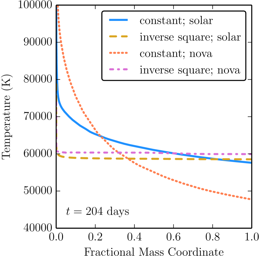
Figure 2.— Temperature profiles of Cloudy simulations of nova ejecta with varying density profiles and compositions. Each represents $10^{-5}\ M_{\odot}$ of ejected material with an outer velocity of 1000 km s^-1 being heated by radiation from a $1.00\ M_{\odot}$ WD SSS. The abscissa measures the total enclosed mass at a given shell radius, with the outermost point being the position enclosing all the mass and a radius of $v_{\mathrm{ej}}t$.

Since Cloudy is inherently a multi-zone code, we can use it to test our assumption that the density profile and composition has little influence on the temperature structure of the ejecta. We ran four models with our fiducial ejecta parameters of $\Delta M_{\mathrm{ej}}=10^{-5}\ M_{\odot}$ and $v_{\mathrm{ej}}=1000\ \mathrm{km\,s^{-1}}$ with the radiation field given by the 1.00 $M_{\odot}$ WD model. These four models used two different density distributions, constant and inverse square, as well as two sets of elemental abundance ratios, solar and nova. The nova abundances are a built-in option in Cloudy and are intended to model the abundanes observed in the ejecta of nova V1500 Cygni (Ferland & Shields, 1978). Since the adiabatic cooling is necessarily radius-dependent for a non-constant density profile, the simple extra cooling of equation (17) could not properly model expansive cooling. To be consistent, we included no extra cooling from expansion in this comparision study, resulting in hotter temperatures and longer “plateau” periods. The temperature profiles of all four cases at a time approximately 200 days after ejection are shown in Figure 2. Importantly, the temperature range changes no more than by order unity in the constant density models and is nearly exactly isothermal in the inverse square cases. Also, the temperatures for these models do not change greatly as the density profile and/or composition are changed, allowing us to use our simple solar composition and constant density assumptions in our semi-analytic model. One important difference between the different density profiles is that the opacity at the lyman-limit diverges as we let the inner radius go to zero in the inverse square case. While a vanishing central radius is certainly unphysical, we must be aware that the time to become optically thick is sensitive to the choice for an inner radius. In this comparison we continued to use $r_{\mathrm{in}}=0.01v_{\mathrm{ej}}t$, which causes the initial optically thick phase to last significantly longer than the similar constant density models, sometimes approaching 100 days.

5. Results

The results of the one zone semi-analytic model and Cloudy simulations for WD mass $0.60,\ 0.80,\ 1.00$, and $1.10\ M_{\odot}$ are shown in Figure 3 and Table 2 from the time-dependent WD models described earlier. All temperatures are in the $10^{4}\mathrm{~{}K}$ region, consistent with that inferred from radio observations and nebular spectroscopy, and show a long plateau of nearly constant temperature at the value expected for photoionization and thermal equilibrium. Results for the two higher-mass WD models are not shown for reasons described below.

Figure 3.— Temperature evolution of the nova ejecta for four WD masses using our semi-analytic model (blue) with cooling curves extracted from Cloudy and simulations run in Cloudy (dashed gold). $\Delta M_{\mathrm{ej}}=10^{-5}\ M_{\odot}$ and $v_{\mathrm{ej}}=1000\ \mathrm{km\,s^{-1}}$ for all models, and the time evolution of the incident radiation is set by the underlying WD mass via the histories shown in Figure 1. The dotted line indicates that the ejecta is optically thick at the Lyman limit edge at early times.

The four WD evolutions shown exhibit a period of isothermal expansion lasting around 100-200 days that we will refer to as the plateau. Numerically, we defined this as the duration over which the the temperature stayed within 20% of the plateau temperature $T_{\rm iso}$. These durations are in accord with the timescale predicted by Equation (16), and show that, even with the WD still providing a high level of photoionization, the adiabatic expansion term eventually plays an important role.

The two methods - one-zone model and Cloudy simulations - agree well for all four cases. The two higher WD mass simulations ($1.20\,M_{\odot}$ and $1.30\,M_{\odot}$) showed much shorter plateau phases (up to $80\mathrm{~{}days}$). However, this was due to the sharp decrease in $T_{\rm eff}$ at early times relative to the 4 lower mass WDs, see Figure 1. The plateau phases were so short in these cases that the ejecta remained optically thick at the photoionization edge throughout and in our model these solutions would not have been self-consistent. For this reason we consider only the WDs in the mass range $0.60-1.10\ M_{\odot}$. Note that for lower ejecta masses and higher ejecta velocities expected of novae on higher-mass WDs, it is possible that the plateau phase would occur after the ejecta has become optically thin. In this work, though, we hold the ejecta parameters constant and thus do not consider the resulting inconsistent results from higher-mass WDs. Most of these results can be motivated and explained by our analytic work that derived equation (16), yielding the dependence of $t_{\rm iso}$ on the ejecta parameters and the average photoelectron energy. Such an understanding will be key to using these observed quantities to constrain either the WD mass or the ejecta properties.

Table 2Isothermal Evolution of Nova Ejecta

$M_{\mathrm{WD}}$		$T_{\mathrm{iso}}$	$t_{\mathrm{iso}}$	$t_{\mathrm{thin}}$
$(M_{\odot})$		($10^{4}$ K)	(d)	(d)
0.60		2.2	229	36
0.80		3.2	155	33
1.00		4.7	152	47
1.10		4.5	217	74

Figure 4.— Ejecta temperature evolution for variations in ejecta velocity (top panel) and ejecta mass (bottom panel). Simulations carried out assuming pure H ejecta with constant $E_{\mathrm{ion}}$ and negligible contribution from collisional ionizations ($P_{\mathrm{ci}}=0$). Unless otherwise indicated $\Delta M_{\rm ej}=10^{-5}~{}M_{\odot}$, $v_{\rm ej}=10^{3}\mathrm{~{}km~{}s^{-1}}$ and $E_{\rm ion}=22$ eV.

Figure 5.— Ejecta temperature evolution for varying average energies of photoelectrons from $4~{}\mathrm{eV}\leq E_{\rm ion}\leq 22~{}\mathrm{eV}$. Simulations carried out assuming pure H ejecta with constant $E_{\mathrm{ion}}$ and negligible contribution from collisional ionizations ($P_{\mathrm{ci}}=0$). Unless otherwise indicated $\Delta M_{\rm ej}=10^{-5}~{}M_{\odot}$, $v_{\rm ej}=10^{3}\mathrm{~{}km~{}s^{-1}}$.

To exhibit this physics, we explored the sensitivity of the plateau phase properties ($T_{\mathrm{iso}}$ and $t_{\mathrm{iso}}$) by varying $v_{\mathrm{ej}}$, $\Delta M_{\mathrm{ej}}$ and $E_{\mathrm{ion}}$ in simulations of a pure H ejecta photoionized by a $1.00~{}M_{\odot}$ WD. We found that variations in ejecta properties ($v_{\mathrm{ej}}$ and $\Delta M_{\mathrm{ej}}$) affect the duration of the plateau but do not alter its temperature. This is revealed in Figure 4 where the ejecta mass varies between $10^{-6}~{}M_{\odot}\lesssim\Delta M_{\rm ej}\lesssim 10^{-4}~{}M_{\odot}$ with velocities in range $10^{2}\mathrm{~{}km\,s^{-1}}\leq v_{\rm ej}\leq 5\times 10^{3}\mathrm{~{}km\,s^{-1}}$. For calculating Figure 4 the $E_{\rm ion}$ was held constant in time for simplicity.

This highlights that the dynamic behavior of the ejecta is described by these two quantities, $v_{\rm ej}$ and $\Delta M_{\mathrm{ej}}$, that we can parametrize into a factor

$$\zeta\equiv\frac{\Delta M_{\mathrm{ej}}}{10^{-5}\ M_{\odot}}\left(\frac{v_{\rm ej}}{10^{3}\ \mathrm{km\,s^{-1}}}\right)^{-3}.$$ (18)

Using Equation (16), $\zeta$ can be inferred from the observed parameters $t_{\mathrm{iso}}$ and $T_{\mathrm{iso}}$ as

$$\zeta(t_{\mathrm{iso}},\ T_{\mathrm{iso}})=\left(\frac{t_{\mathrm{iso}}}{250\ \mathrm{d}}\right)^{2}\left(\frac{kT_{\mathrm{iso}}}{1\mathrm{~{}eV}}\right)\times\\ \left(\frac{E_{\rm ion}}{10\mathrm{~{}eV}}\right)^{-1}\left(\frac{\alpha}{10^{-13}\ \mathrm{cm^{3}\,s^{-1}}}\right),$$ (19)

potentially yielding insights into the ejecta properties from observations. The average photo-electron energy $E_{\rm ion}$ depends on the WD’s $T_{\rm eff}$ and is the main determinant of $T_{\rm iso}$, as is evident in Figure 5. Hence, the plateau temperature is most sensitive to the WD $T_{\rm eff}$ (and hence WD mass).

The plateau phase space behavior of $\zeta$ is shown in Figure 6 with dashed lines of constant $\zeta$. For nearly all cases, we see that $T_{\mathrm{iso}}$ is highly independent of the ejecta information, $v_{\mathrm{ej}}$ and $\Delta M_{\mathrm{ej}}$. This implies that changes made to the dynamic properties of the ejecta should be relatively insignificant for the temperature, making it a potentially clean diagnostic for WD mass. This also implies that changes to the ejecta profile (e.g. non-spherically symmetric ejections) or homogeneity would unlikely impact $T_{\rm iso}$.

The thermal evolution of the ejecta at late times is simple if the SSS phase has ended, as the ejecta undergoes an adiabatic temperature decline, and $T\propto t^{-2}$ thereafter. The recombination time is far longer than the age when $t>t_{\rm iso}$, so that this plasma would maintain itself in a highly ionized state even though photoionization has ended. Hence, it would still be a thermal bremsstrahlung radio emitter during the adiabatic decline. If the SSS remains on at $t>t_{\rm iso}$, we can still approximate the thermal evolution. In this limit, photoionization heating is still operative, so the temperature decline would not be as steep as the adiabatic relation. Rather, for the cases we considered here, the photoionization timescale is still much less than the age, $t_{\rm ion}\ll t$, so that the heating remains operative, and the required small neutral fraction is easily maintained. If we assume negligible radiative cooling, rather safe as $T<10^{4}$ K, then equation (15) simplifies to an integrable form. If the ejecta temperature was $T_{0}$ at $t=t_{0}$, then its value at a time $t>t_{\rm iso}$ is simply

$${T\over T_{0}}\approx{t_{0}^{2}\over t^{2}}\exp\left({t_{\rm iso}^{2}\over t_{0}^{2}}-{t_{\rm iso}^{2}\over t^{2}}\right),$$ (20)

exhibiting the less steep than adiabatic decline that is evident in nearly all our results. Differentiating between a decline from SSS shutoff versus onset of dominance of adiabatic expansion with an active photoionization source could be attempted by comparing $T(t)$ inferred from radio observations or nebular spectroscopy to $T\propto t^{-2}$ versus the more complicated relation of equation (20). Alternatively, a shut-off of the X-ray source could be confirmed by direct measurements like those of Schwarz et al. (2011) and Henze et al. (2011, 2014b). Equation (20) assumes a constant ionizing source, but the WD models used in Figure 3 are still increasing in effective temperature when adiabatic expansion takes over, so their decline is even less steep then equation (20) would indicate.

Figure 6.— Characteristic plot of the plateau phase with dotted lines of constant ejecta parameter $\zeta=10^{14}\times\frac{\Delta M_{\mathrm{ej}}}{v_{\rm ej}^{3}}$ spaced evenly in log space. A line of a particular color connects models of identical WD mass.

6. Conclusions

We have shown that the photoionizing emission from the hot white dwarf following a classical nova is adequate to explain the inferred ejecta temperatures $>10^{4}$ K that persist for nearly a year after the optical outburst. For the typical WD mass, $\approx 0.8M_{\odot}$, of a CNe this nearly isothermal phase lasts for about one year (see equation (16)) and has a temperature of $T\approx(2-3)\times 10^{4}$ K, in good agreement with many observed novae. Even when the SSS phase lasts for decades, the balance between heating and cooling eventually ends, and the ejecta transitions into a phase of temperature decline roughly approximated analytically by equation (20). If the SSS phase ends early, then the ejecta temperature would evolve adiabatically, as $T\propto t^{-2}$.

Though our preliminary calculations allow us to see the basics of how photoionization heating is balanced by cooling at early times, and how the heating is weak compared to adiabatic expansive effects at late times, work remains to realize the quantitative accuracy adequate to infer CNe ejecta properties or WD masses. We certainly identified a degeneracy in how the ejecta information ($\Delta M_{\mathrm{ej}}$ and $v_{\mathrm{ej}}$) affect the plateau phase duration, which should allow observers to make predictions about the properties of a given nova, complementing existing radio techniques (Seaquist & Palimaka, 1977; Hjellming et al., 1979; Heywood et al., 2005). For example, equation (19) makes possible the inference of an ejecta mass range based on the length of the isothermal temperature evolution inferred in the radio combined with the measured velocity of the ejecta and temperature.

However, specific events would be best modeled by a unique Cloudy simulation that reflects the known properties of the event as inferred from the optical, as well as the X-ray supersoft phase. That would also allow for inclusion of unusual abundances constrained from modeling the nebular spectroscopy as in Schwarz (2002), Vanlandingham et al. (2005), and Schwarz et al. (2007), which would in turn impact the mapping of the observed ejecta temperature to the WD mass. The ideal calcuation could use a more realistic ejecta density profile, like a Hubble flow (Seaquist & Palimaka, 1977) with an appropriate filling factor, though our efforts imply that the ejecta temperature is relatively independent of the specific density structure for the first year or so. We hope that the expanded efforts with the Karl G. Jansky Very Large Array to monitor nearby galactic novae will enable a new era of quantitative analysis of the late time radio observations (Roy et al., 2012).

We thank Laura Chomiuk, Tommy Nelson, Jeno Sokoloski and Dean Townsley for discussions on the radio observations that inspired our efforts, and Orly Gnat for advice on using Cloudy. We also thank our referee, Steve Shore, for his many helpful insights that improved the paper. This work was supported by the National Science Foundation under grants PHY 11-25915, AST 11-09174, and AST 12-05574. Most of the MESA simulations for this work were made possible by the Triton Resource, a high-performance research computing system operated by the San Diego Supercomputer Center at UC San Diego. We are also grateful to Bill Paxton for his continual development of MESA.

References

- Austin et al. (1996) Austin, S. J., Wagner, R. M., Starrfield, S., et al. 1996, Astronomical Journal v.111, 111, 869
- Baker & Menzel (1938) Baker, J. G., & Menzel, D. H. 1938, ApJ, 88, 52
- Beck et al. (1990) Beck, H., Gail, H. P., Gass, H., & Sedlmayr, E. 1990, Astronomy and Astrophysics (ISSN 0004-6361), 238, 283
- Draine (2011) Draine, B. T. 2011, Physics of the Interstellar and Intergalactic Medium by Bruce T. Draine. Princeton University Press
- Eyres et al. (1996) Eyres, S. P. S., Davis, R. J., & Bode, M. F. 1996, MNRAS, 279, 249
- Ferland & Shields (1978) Ferland, G. J., & Shields, G. A. 1978, ApJ, 226, 172
- Ferland et al. (2013) Ferland, G. J., Porter, R. L., van Hoof, P. A. M., et al. 2013, Revista Mexicana de Astronomía y Astrofísica Vol. 49, 49, 137
- Fujimoto (1982) Fujimoto, M. Y. 1982, ApJ, 257, 767
- Gallagher & Starrfield (1978) Gallagher, J. S., & Starrfield, S. 1978, ARA&A, 16, 171
- Hachisu & Kato (2010) Hachisu, I., & Kato, M. 2010, ApJ, 709, 680
- Henze et al. (2014a) Henze, M., Ness, J. U., Darnley, M. J., et al. 2014a, A&A, 563, L8
- Henze et al. (2011) Henze, M., Pietsch, W., Haberl, F., et al. 2011, A&A, 533, 52
- Henze et al. (2014b) —. 2014b, A&A, 563, 2
- Heywood et al. (2005) Heywood, I., O’Brien, T. J., Eyres, S. P. S., Bode, M. F., & Davis, R. J. 2005, MNRAS, 362, 469
- Hjellming et al. (1979) Hjellming, R. M., Wade, C. M., Vandenberg, N. R., & Newell, R. T. 1979, AJ, 84, 1619
- Krautter (2008) Krautter. 2008, Classical Novae, 2nd edn., ed. M. F. Bode & A. Evans (Cambridge University Press), 232–251
- Lang (1980) Lang, K. R. 1980, Astrophysical Formulae: a compendium for the physicist and astrophysicist, 2nd edn. (Berlin ; New York : Springer-Verlag)
- MacDonald & Vennes (1991) MacDonald, J., & Vennes, S. 1991, ApJ, 373, L51
- Ness et al. (2008) Ness, J. U., Schwarz, G., Starrfield, S., et al. 2008, AJ, 135, 1328
- Oegelman et al. (1984) Oegelman, H., Beuermann, K., & Krautter, J. 1984, ApJ, 287, L31
- Paxton et al. (2011) Paxton, B., Bildsten, L., Dotter, A., et al. 2011, ApJS, 192, 3
- Paxton et al. (2013) Paxton, B., Cantiello, M., Arras, P., et al. 2013, ApJS, 208, 4
- Roy et al. (2012) Roy, N., Chomiuk, L., Sokoloski, J. L., et al. 2012, Bulletin of the Astronomical Society of India, 40, 293
- Sala & Hernanz (2005) Sala, G., & Hernanz, M. 2005, A&A, 439, 1061
- Schwarz (2002) Schwarz, G. J. 2002, ApJ, 577, 940
- Schwarz et al. (2007) Schwarz, G. J., Shore, S. N., Starrfield, S., & Vanlandingham, K. M. 2007, ApJ, 657, 453
- Schwarz et al. (2011) Schwarz, G. J., Ness, J.-U., Osborne, J. P., et al. 2011, ApJS, 197, 31
- Seaquist & Bode (2008) Seaquist, E. R., & Bode, M. F. 2008, Classical Novae, 2nd edn., ed. M. F. Bode & A. Evans (Cambridge University Press), 141–166
- Seaquist & Palimaka (1977) Seaquist, E. R., & Palimaka, J. 1977, ApJ, 217, 781
- Shore (2008) Shore, S. N. 2008, Classical Novae, 2nd edn., ed. M. F. Bode & A. Evans (Cambridge University Press), 194–231
- Shore et al. (2013) Shore, S. N., Schwarz, G. J., De Gennaro Aquino, I., et al. 2013, A&A, 549, A140
- Starrfield et al. (2008) Starrfield, S., Iliadis, C., & Hix, W. R. 2008, Classical Novae, 2nd edn., ed. M. F. Bode & A. Evans (Cambridge University Press), 77–101
- Starrfield et al. (1974) Starrfield, S., Sparks, W. M., & Truran, J. W. 1974, ApJS, 28, 247
- Tang et al. (2014) Tang, S., Bildsten, L., Wolf, W. M., et al. 2014, ApJ, 786, 61
- Taylor et al. (1988) Taylor, A. R., Hjellming, R. M., Seaquist, E. R., & Gehrz, R. D. 1988, Nature (ISSN 0028-0836), 335, 235
- Vanlandingham et al. (2005) Vanlandingham, K. M., Schwarz, G. J., Shore, S. N., Starrfield, S., & Wagner, R. M. 2005, ApJ, 624, 914
- Wolf et al. (2013) Wolf, W. M., Bildsten, L., Brooks, J., & Paxton, B. 2013, ApJ, 777, 136