Identification of a Hybrid Spring Mass Damper via Harmonic Transfer Functions as a Step Towards Data-Driven Models for Legged Locomotion

Abstract

There are limitations on the extent to which manually constructed mathematical models can capture relevant aspects of legged locomotion. Even simple models for basic behaviours such as running involve non-integrable dynamics, requiring the use of possibly inaccurate approximations in the design of model-based controllers. In this study, we show how data-driven frequency domain system identification methods can be used to obtain input–output characteristics for a class of dynamical systems around their limit cycles, with hybrid structural properties similar to those observed in legged locomotion systems. Under certain assumptions, we can approximate hybrid dynamics of such systems around their limit cycle as a piecewise smooth linear time periodic system (LTP), further approximated as a time-periodic, piecewise LTI system to reduce parametric degrees of freedom in the identification process. In this paper, we use a simple one-dimensional hybrid model in which a limit-cycle is induced through the actions of a linear actuator to illustrate the details of our method. We first derive theoretical harmonic transfer functions of our example model. We then excite the model with small chirp signals to introduce perturbations around its limit-cycle and present systematic identification results to estimate the harmonic transfer functions for this model. Comparison between the data-driven HTF model and its theoretical prediction illustrates the potential effectiveness of such empirical identification methods in legged locomotion.

I Introduction

Legged locomotion emerges from a staggering diversity of animal and robot morphologies and gaits, and modeling locomotor dynamics remains a grand challenge in both biology and robotics [1, 2]. Running behaviors, in particular, are commonly represented by relatively simple spring–mass models such as the Spring-Loaded Inverted Pendulum (SLIP) model [3, 4]. A common feature of such models, however, is that their hybrid system dynamics involve intermittent foot contact with the ground, alternating between flight and stance phases during locomotion. Despite the presence of seemingly simple models for basic behaviors such as running and walking, the hybrid dynamics associated with these behaviors can be rather complex, with non-integrable parts such as the stance phase [5, 3]. Given the utility of having accurate models and associated analytic solutions in constructing high performance controllers for nonlinear systems, substantial effort has been devoted to the construction of approximate solutions to such non-integrable hybrid models [6, 7, 8, 9].

When accurate analytical solutions to the dynamics of a legged platform are available [8], their structure can be exploited to yield effective solutions for system identification and adaptive control [10]. Despite our previous studies showing how accurate such models may be, there will always be unmodeled components in the physical system, resulting in discrepancies between the model and experiments [11]. Attempts to manually incorporate these effects into the model is daunting at best, and often impossible. Consequently, we propose an alternative method in this study, namely using data-driven system identification methods to derive an input–output transfer function for such hybrid legged locomotion behaviors, thereby eliminating the need to manually construct an explicit mathematical model for the system.

Our main goal in this study is to provide a system identification framework applicable to a useful (although not comprehensive) class of legged locomotion models [8], and possibly more complex robotic systems [12]. Our approach is based on considering legged locomotion as a hybrid nonlinear dynamical system with a stable periodic orbit (limit-cycle), corresponding to the locomotor behavior of interest. We introduce a formulation that addresses the input–output system identification problem in the frequency domain for a sub-class of hybrid legged locomotion models. More specifically, following certain assumptions on the hybrid dynamics of legged systems, we approximate their hybrid dynamics around the limit-cycle as a linear time-periodic system (LTP). However, this first LTP approximation is infinite dimensional, making parametric identification challenging. We hence further approximate the dynamics as a finite dimensional piecewise LTI system (maintaining its LTP nature), thereby limiting the parametric degrees of freedom while enabling a practical identification framework.

Existing studies on system identification of LTP systems focus on modeling these systems as multi-input single-output LTI systems. This approach is based on the concept of harmonic transfer functions [13], which are infinite-dimensional operators that are analogous to frequency response functions for LTI systems. An identification strategy for such systems was developed in [14] using power spectral density and cross spectral density functions. A similar method was used in [15] considering the effects of noise in both input and output measurements. Different than these studies, local polynomial methods and lifting approaches were also used for the identification of harmonic transfer functions for multi-input single-output models of LTP systems [16].

Our contributions in this paper focus on representing the dynamics of legged locomotion as a linear time periodic system, thereby enabling the use of the system identification method proposed in [14] for such systems. We achieve this by using a new phase definition in identifying the harmonic transfer functions, illustrated in the context of a simplified model designed to mirror structural properties of legged locomotion models. When the problem is approached as a grey-box model with finite parameters (piecewise LTI), it suffices to non-parametrically estimate a finite number of harmonics, to which we later fit parametric models.

Ankarali and Cowan [17] developed a similar system identification method for hybrid systems with periodic orbits using “discrete time” harmonic transfer functions. However, the framework and assumptions in this paper are distinctly different from their approach. Specifically, they use mappings between different cross sections to construct a discrete-time LTP system, and use discrete time HTFs for identification. Also, the current paper focuses on harmonic balance, which also distinguishes this paper from [17].

II Representation of Legged Locomotion as a Hybrid Dynamical System

Our goal in this study is to provide a system identification framework for a class of models related to legged locomotion using harmonic transfer functions. For the present paper, we limit ourselves to “clock-driven” locomotion models as described in Section II-A, representative of controllers used by a wide variety of existing robots [12, 18, 19], with open-loop central pattern generators (CPG) coordinating control actions to achieve time periodic behaviour. This will allow us to directly use time periodicity in our LTP analysis, while eliminating a variety of complications associated with estimating the phase [20].

II-A Smooth Clock-driven Oscillators

In general, the dynamics of smooth, clock-driven oscillators with external inputs can be written as

$$\begin{aligned} \dot{q}&=f(q,\phi,u),\\ \dot{\phi}&=1\\ f&:\mathbb{R}^{n}\times S^{1}\times\mathbb{R}^{p}\mapsto\mathbb{R}^{n}\\ (q,\ \phi)&\in\ \mathbb{R}^{n}\times S^{1},\ u\in\mathbb{R}^{q}\end{aligned}$$ (1)

where $(q,\phi)$ and $\mathbb{R}^{n}\times S^{1}$ denote the state vector and the state space of the oscillator, respectively. The circle component $S^{1}=\mathrm{mod}(\mathbb{R}^{+},T)$ enforces the periodicity of the dynamics, while the external input $u(t)$ represents small external perturbations which we will use for system identification.

In this paper, we focus on oscillators of the form (1) with asymptotically stable, isolated periodic orbits (limit-cycle) $\bar{q}(t)=\bar{q}(t-T)$ when $u(t)=0$. For such systems, if we let $q(t)=\bar{q}(t)+x(t)$ and linearize the dynamics in (1) around the limit-cycle $\bar{q}(t)$, and $u(t)=0$ we get

$$\begin{aligned} \dot{x}(t)=A(t)x(t)+B(t)u(t)\\ y(t)=C(t)x(t)+D(t)u(t)\end{aligned}$$ (2)

where

$$A(t) = \left[\frac{\partial f}{\partial q}\right]_{\begin{smallmatrix}q(t)&=&\bar{q}(t)\\ u(t)&=&0\end{smallmatrix}},$$ (3)

$$B(t) = \left[\frac{\partial f}{\partial u}\right]_{\begin{smallmatrix}q(t)&=&\bar{q}(t)\\ u(t)&=&0\end{smallmatrix}}.$$ (4)

This corresponds to a Linear Time Periodic (LTP) system, with all system matrices sharing a common period, $T$.

II-B Modeling Framework for Hybrid Systems

Legged systems are often modeled using hybrid dynamics due to intermittent foot contact with the ground, which cannot be represented with a single, smooth dynamical flow. In the broadest sense, a hybrid dynamical system is a set of smooth flows together with discrete transitions (and associated transformations) between these flows triggered by intersections of system trajectories with sub-manifolds of the continuous state space [21]. These flows are called charts, indexed with unique labels $\mathcal{I}:=\{0,\cdots,d\}$ each with possibly different equations of motion. Along its trajectories, a hybrid system transitions from one chart to another, with each transition defined by the zero crossing of a threshold function. For each source chart $\alpha\in\mathcal{I}$ and destination chart $\beta\in\mathcal{I}$, the threshold function $h_{\alpha}^{\beta}$ defines the transition from chart $\alpha$ to chart $\beta$. An example transition graph for a hybrid dynamical system is illustrated in Fig. 1.

Figure 1: A simple state transition graph for a hybrid dynamical system.

Since we are interested in the local behaviour around the limit-cycle, we assume that there is only one transition function associated with each chart. We further assume that system trajectories are continuous at transitions, meaning that system states do not experience discrete changes coincident with chart transitions. As a final note, we assume that the hybrid dynamical system we consider has an isolated periodic orbit ensuring that chart transitions within the limit cycle are also periodic and consistent.

It is important to note that these assumptions are generally satisfied by models of common locomotory behaviors such as running and walking [8, 22] as well as a wide range of legged robots for which leg masses are negligible compared to the dynamics of a larger body [12, 18]. Consequently, the system identification methods we introduce will remain applicable to systems other than the simplified example we will present in this paper.

II-C Modeling Legged Locomotion as a Linear Time Periodic System

For clarity, we limit our focus in this section to an example hybrid dynamical system with only two charts, $\mathcal{I}=\{0,1\}$, designed to capture stance and flight phases of simple spring-mass models of locomotion. Based on a clock driven assumption, for each $i\in\mathcal{I}$ the continuous dynamics can be represented with

$$\begin{aligned} \dot{\phi}&=1\\ \dot{q}_{i}&=f_{i}(q,\phi,u)\ ,\ \\ q_{i}&\in\mathbb{R}^{n}\end{aligned}$$ (5)

and let the associated threshold function be $h_{i}^{\mathrm{mod}(i+1,2)}(q)$. The transition map associated with each hybrid event is simply the identity map, $q_{i}\mapsto q_{i}$, due to the continuity assumption. Our linearization of these hybrid dynamics towards an LTP approximation assumes that these transition times, $\hat{t}$, zero crossings of $h_{0}^{1}(q)$ and $h_{1}^{0}(q)$, maintain their periodicity and offsets within the period in close proximity of the limit-cycle, resulting in the following form of the nonlinear dynamics

$$\dot{\phi} =1$$ (6)

$$\dot{q} \approx\left\{\begin{aligned} &f_{0}(q,\phi,u)\ ,\ \mathrm{if}\ \mathrm{mod}(t,T)\in[0,\hat{t})\\ &f_{1}(q,\phi,u)\ ,\ \mathrm{if}\ \mathrm{mod}(t,T)\in[\hat{t},T)\end{aligned}\right.\;.$$ (7)

Assuming that the system given above has a limit cycle $\bar{q}(t)$ with a period $T$, linearization around $\bar{q}(t)$ yields the piecewise smooth LTP system

$$\begin{aligned} \dot{x}(t)&=\left\{\begin{aligned} &A_{0}(t)x(t)+B_{0}(t)u(t),\ \mathrm{if}\ \mathrm{mod}(t,T)\in[0,\hat{t})\\ &A_{1}(t)x(t)+B_{1}(t)u(t),\ \mathrm{if}\ \mathrm{mod}(t,T)\in[\hat{t},T)\end{aligned}\right.\end{aligned}$$

where

$$\begin{aligned} A_{0}(t):=\left[\frac{\partial f_{0}}{\partial q}\right]_{\begin{smallmatrix}q(t)&=&\bar{q}(t)\\ u(t)&=&0\end{smallmatrix}},B_{0}(t):=\left[\frac{\partial f_{0}}{\partial u}\right]_{\begin{smallmatrix}q(t)&=&\bar{q}(t)\\ u(t)&=&0\end{smallmatrix}},\\ A_{1}(t):=\left[\frac{\partial f_{1}}{\partial q}\right]_{\begin{smallmatrix}q(t)&=&\bar{q}(t)\\ u(t)&=&0\end{smallmatrix}},B_{1}(t):=\left[\frac{\partial f_{1}}{\partial u}\right]_{\begin{smallmatrix}q(t)&=&\bar{q}(t)\\ u(t)&=&0\end{smallmatrix}}.\end{aligned}$$

It is natural to assume that direct measurement of all $x(t)$ may not be available or we may only measure a subset of $x(t)$. Consequently, we also define a time-periodic output equation as in the form (9).

Since system matrices $A_{i}(t)$, $B_{i}(t)$, $C_{i}(t)$ and $D_{i}(t)$ with $i\in\{0,1\}$ are time parametrized functions, the system has infinite parametric degrees of freedom, making parametric system identification challenging even when Harmonic Transfer Functions are used. At this point, we hypothesize that for hybrid systems, the variability within a chart is small compared to the change between charts and we approximate the LTP dynamics using a piecewise LTI approximation that preserves the LTP structure of the system. The LTP equations of motion then take the form

$$\begin{aligned} \dot{x}(t)&\approx\left\{\begin{aligned} &A_{0}x(t)+B_{0}u(t),\ \mathrm{if}\ \mathrm{mod}(t,T)\in[0,\hat{t})\\ &A_{1}x(t)+B_{1}u(t),\ \mathrm{if}\ \mathrm{mod}(t,T)\in[\hat{t},T)\end{aligned}\right.\end{aligned}$$ (8)

$$\begin{aligned} y(t)&\approx\left\{\begin{aligned} &C_{0}x(t)+D_{0}u(t),\ \mathrm{if}\ \mathrm{mod}(t,T)\in[0,\hat{t})\\ &C_{1}x(t)+D_{1}u(t),\ \mathrm{if}\ \mathrm{mod}(t,T)\in[\hat{t},T)\end{aligned}\right.\end{aligned}$$ (9)

The formulation above constitutes the basis of our framework for analyzing and identifying clock-driven legged locomotion models.

III Harmonic Transfer Functions

III-A Preliminaries and Background

System identification studies on (stable) LTI systems rely on the fact that if the input is sinusoidal, then, at steady-state, the output will also be a sinusoidal signal (at the same frequency but with a possibly different magnitude and phase). This one-to-one mapping between input and output signals allows us to characterize the dynamics in terms of a frequency response function (FRF) also know as a Bode plot. Unfortunately, this approach does not readily transfer to LTP systems, which produce output spectra that include multiple (possibly infinite) harmonics of the input stimuli, each with possibly different magnitude and phase at steady state.

One ad hoc way to mitigate this is to enforce a one-to-one mapping by neglecting higher harmonics [23]. However, this assumption may result in substantial inaccuracies particularly when the influence of higher harmonics on the response is expected to be significant. Motivated by this problem, Wereley [24] proposed a linear one-to-one mapping between the coefficients of an exponentially modulated periodic (EMP) signal at the input of LTP systems to the coefficients of an EMP signal at their output. This linear operator that maps the input harmonics to the output harmonics of an LTP system is called a Harmonic Transfer Function (HTF) [13].

In the following section, we review the derivation of harmonic transfer functions as presented in [13] and [25], using the principle of harmonic balance starting from the state space representation of (2).

III-B Theoretical Derivation of Harmonic Transfer Functions

Recall that the system matrices in (2) are all $T$-periodic. Consequently, they can be represented by an infinite Fourier series with pumping frequency $\omega_{p}=2\pi/T$. For the system matrix $A(t)$, we have

$$A(t)=\sum\limits_{n=-\infty}^{\infty}A_{n}e^{j\omega_{p}nt}\;.$$ (10)

The matrices $B(t)$, $C(t)$ and $D(t)$ can be similarly decomposed. In addition, we can also expand the state and output vectors since they are both EMP signals. Substituting these expansions into (2) and applying the principle of harmonic balance as explained in [13], we obtain the harmonic state space representation as

$$s\mathcal{X} =(\mathcal{A}-\mathcal{N})\mathcal{X}+\mathcal{B}\mathcal{U}$$ (11)

$$\mathcal{Y} =\mathcal{C}\mathcal{X}+\mathcal{D}\mathcal{U},$$

where the doubly infinite vectors representing the harmonics of the state, control, and output signals are

$$\mathcal{X}^{T} :=[\cdots,x_{-2}^{T},x_{-1}^{T},x_{0}^{T},x_{1}^{T},x_{2}^{T},\cdots],$$ (12)

$$\mathcal{U}^{T} :=[\cdots,u_{-2}^{T},u_{-1}^{T},u_{0}^{T},u_{1}^{T},u_{2}^{T},\cdots],$$

$$\mathcal{Y}^{T} :=[\cdots,y_{-2}^{T},y_{-1}^{T},y_{0}^{T},y_{1}^{T},y_{2}^{T},\cdots],$$

and the doubly infinite input modulation matrix is

$$\mathcal{N}:=\mathrm{blockdiag}\{jn\omega_{p}I\},\indent\forall n\in Z,$$ (13)

which modulates the input frequency to different harmonic frequencies. Details on the derivations can be found in [13].

The $T$-periodic dynamics matrix, $A(t)$, is expressed in terms of its complex Fourier coefficients, $\{A_{n}|n\in\mathbb{Z}\}$, as a doubly infinite block Toeplitz matrix,

$$\mathcal{A}=\begin{bmatrix}\ddots&\vdots&\vdots&\vdots&\vdots&\vdots&\\ \cdots&A_{0}&A_{-1}&A_{-2}&A_{-3}&A_{-4}&\cdots\\ \cdots&A_{1}&A_{0}&A_{-1}&A_{-2}&A_{-3}&\cdots\\ \cdots&A_{2}&A_{1}&A_{0}&A_{-1}&A_{-2}&\cdots\\ \cdots&A_{3}&A_{2}&A_{1}&A_{0}&A_{-1}&\cdots\\ \cdots&A_{4}&A_{3}&A_{2}&A_{1}&A_{0}&\cdots\\ &\vdots&\vdots&\vdots&\vdots&\vdots&\ddots\end{bmatrix},$$ (14)

with a similar definition for $B(t)$ in terms of its Fourier coefficients represented by $\{B_{n}|n\in\mathbb{Z}\}$, $C(t)$ in terms of $\{C_{n}|n\in\mathbb{Z}\}$, and $D(t)$ in terms of $\{D_{n}|n\in\mathbb{Z}\}$.

This collection of doubly infinite matrices is called the harmonic state space model ($\mathcal{HSS}$) of the system given in (2). However, it will also be useful to determine an explicit input–output functional relationship between the Fourier coefficients of the harmonics of the input, $\{u_{n}|n\in\mathbb{Z}\}$, and those of the output, $\{y_{n}|n\in\mathbb{Z}\}$. This relationship is represented by the harmonic transfer function, ${G}(s)$, which is also an infinite dimensional matrix of Fourier coefficients, satisfying

$$\mathcal{Y}={G}\mathcal{U}\;.$$ (15)

Based on (11), ${G}$ can be computed as

$${G}=\mathcal{C}[sI-(\mathcal{A-N})]^{-1}\mathcal{B}+\mathcal{D}\;,$$ (16)

as long as the inverse within this equation exists.

There are, however, two problems associated with the harmonic transfer function as stated above. First, it is not clear whether the inverse of the doubly infinite matrix in the definition of the harmonic transfer function will always exist. This problem will be dealt with by an application of the Floquet Theorem. Second, the harmonic transfer function is a doubly infinite matrix operator, which cannot practically be implemented on a computer. This second problem will be mitigated by truncating the HTF in order to implement analysis on a computer.

Note that the theoretical definition of harmonic transfer functions in [13], reviewed in this section, requires the state space representation of the system to be available. Our goal is to estimate this theoretically computed transfer function ${G}(s)$ by using input-output data in the frequency domain without necessitating knowledge of internal system dynamics.

III-C Estimation of Harmonic Transfer Functions via Frequency Domain System Identification

In this section, we briefly explain the data-driven system identification method presented in [14].

In an LTP system, a sinusoidal input at a specific frequency generates a superposition of sinusoids at multiple (possibly an infinite number of) harmonics. Consequently, the system identification framework starts with truncating the number of harmonic transfer functions ${\hat{G}}$ to be estimated. In the following examples, we consider only three frequencies in the output to clearly illustrate the approach of [14].

Suppose that an LTP system consists of the superposition of three different harmonic transfer functions, ${\hat{G}}_{0}$, ${\hat{G}}_{-1}$ and ${\hat{G}}_{1}$, each corresponding to a different frequency component of the output. The output can then be expressed as

$$\hat{Y}(j\omega) = {\hat{G}}_{0}(j\omega)U(j\omega)+{\hat{G}}_{-1}(j\omega)U(j\omega+j\omega_{p})$$ (17)

$$+{\hat{G}}_{1}(j\omega)U(j\omega-j\omega_{p}).$$

In this new formulation, the $n^{th}$ transfer function is defined as the linear operator that maps the output at frequency $\omega$ to an input at the same frequency, modulated with $e^{jn\omega_{p}t}$. However, a single input–output pair in each frequency will naturally not be sufficient to estimate harmonic transfer functions as in the case of LTI systems, since the identification problem will then be underdetermined. Therefore, either at least three independent inputs or additional constraints must be provided to enable a successful identification of these harmonic transfer functions.

There are two key issues that need to be addressed before designing input signals for the identification process. First, we will require the use of at least as many variations on the input signal as the number of harmonic transfer functions to be estimated. This is accomplished in [14], which uses a single input sequence signal for system identification, constructed by concatenating phase shifted copies of a single waveform on the input evenly separated by delays within the system period. A complete characterization of system dynamics is possible with this method since different modes of the system were activated through the use of phase-shifted copies of a single waveform.

The second issue is the need to excite all frequency components within the system by providing input signals with a sufficiently wide frequency spectrum. This can be accomplished through the use of chirp signals, whose frequency varies with time. The use of chirp input signals, combined with the idea of supplying multiple, phase-shifted input sequences allows us to obtain sufficiently rich input–output data to support the system identification process.

Using this data with input–output pairs, one can estimate the harmonic transfer functions of the system, so that the error between actual and estimated outputs is minimized. Therefore, we can convert the identification problem to an optimization formulated as

$$\underset{\mathbf{\hat{G}}}{\text{minimize}} \mathbf{J}=(\mathbf{Y}-\mathbf{U}^{\mathbf{T}}\mathbf{\hat{G}})^{2}.$$ (18)

However, note that Siddiqi [14] combines all phase-shifted signals in a single input. Hence, the problem is still underdetermined in the frequency domain, since a single input–output pair for a specific frequency will not be sufficient to identify three harmonic transfer functions. In order to address this problem, they consider additional constrains on the estimated harmonic transfer functions. First, they assume that transfer functions are smooth, which is reasonable for physical systems. This is enforced through a difference operator, $\mathbf{D^{2}}$, designed to compute the second derivative of a vector when multiplied from the left side. Details on the derivations for $\mathbf{D^{2}}$ can be found in [14].

The smoothness condition on transfer functions requires penalizing the curvature of individual transfer functions. Therefore, [14] modifies (LABEL:eq:costfunc1) to include a cost associated with the curvature, yielding a revised minimization problem formulated as

$$\underset{\mathbf{\hat{G}}}{\text{minimize}} \mathbf{J}=(\mathbf{Y}-\mathbf{U}^{\mathbf{T}}\mathbf{\hat{G}})^{2}+(\alpha\mathbf{D^{2}}\mathbf{\hat{G}})^{2}\;,$$ (19)

where $\alpha$ is a manually tuned constant weight for penalizing curvature. The solution of (LABEL:eq:costfunc2) can easily be obtained by differentiating $\mathbf{J}$ with respect to $\mathbf{\hat{G}}$, taking the form

$$\mathbf{\hat{G}}=(\mathbf{U}^{\mathbf{T}}\mathbf{U}+\alpha\mathbf{D^{4}})^{-1}\mathbf{U}^{\mathbf{T}}\mathbf{Y}\;,$$ (20)

where the rows of the matrix $\mathbf{\hat{G}}(\omega)$ correspond to individual different harmonic transfer functions as

$$\mathbf{\hat{G}}(\omega)=\begin{bmatrix}\mathbf{\hat{G}}_{1}(\omega)\\ \mathbf{\hat{G}}_{0}(\omega)\\ \mathbf{\hat{G}}_{-1}(\omega)\\ \end{bmatrix}.$$ (21)

Note that $\mathbf{U}^{\mathbf{T}}\mathbf{U}$ and $\mathbf{U}^{\mathbf{T}}\mathbf{Y}$ correspond to power spectral and cross spectral density functions, respectively. Therefore, (20) is analogous to estimating transfer functions in LTI systems, with an additional cost on curvature.

IV Simplified Legged Locomotion Model with Hybrid System Dynamics

In this section, we describe a simple, vertically constrained spring-mass-damper system that possesses hybrid structural properties similar to the extensively studied Spring-Loaded Inverted Pendulum (SLIP) model for running behaviors. This will provide a simple example to illustrate the application of our system identification method to such systems.

IV-A System Dynamics

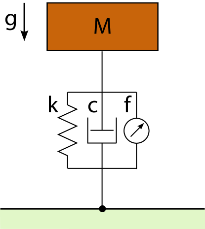
Figure 2: Simplified leg model.

Fig. 2 illustrates the vertical leg model we focus on in this section. It consists of a mass attached to a leg with a spring-damper mechanism as well as a force transducer. Unlike the SLIP model, we assume that the toe is permanently affixed on the ground. Nevertheless, we recover the hybrid nature of locomotory gaits by assuming that the damper is turned on during a “stance phase” (lossy) and off during a “flight phase” (lossless). This construction recovers the hybrid nature of the dynamics, while allowing active input throughout the entire trajectory to support the generation of system identification data, as well as admitting theoretical computation of its harmonic transfer functions for a comparative investigation.

We use the force transducer $f$ in this system for two purposes. Firstly, active energy input to the system must be provided to maintain the limit cycle and compensate for energy losses due to the presence of damping. Second, it will be used as an exogenous input to the system to support the system identification process. Many physical legged platforms include similar active components in their legs to regulate their mechanical energy [26, 27]. Notwithstanding differences in how these actuators are incorporated into the system, they can all be used as the necessary exogenous inputs to perform system identification. A similar model was also investigated in [16] but using an additional nonlinear spring for energy regulation.

The equations of motion for this simplified legged locomotion model are given by

$$m\ddot{x}=\begin{cases}-mg-c\dot{x}-k(x-x_{0})+f(t),&\text{if }\dot{x}>0\\ -g-k(x-x_{0})+f(t),&\text{otherwise}.\end{cases}$$ (22)

The lossy and lossless dynamics in (22) correspond to different charts in Fig. 1 and zero crossings of $\dot{x}$ represent threshold functions for both phases.

Our illustrative examples use the parameters $g=9.81$, $k=200$, $c=2$, $m=1$ and $x_{0}=0.2$, chosen to be similar to the parameters of a vertical hopper platform in our laboratory [28]. As noted above, we choose the linear actuator input $f(t)=f_{0}(t)+u(t)$, consisting of a forcing term $f_{0}(t)$ to compensate for energy losses, and a chirp signal $u(t)$ to introduce small periodic perturbations for system identification.

IV-B Theoretical Computation of Harmonic Transfer Functions

The goal of this section is to compute harmonic transfer functions for our model around its limit cycle as outlined in Section III-B.

We first assume that the forcing input $f_{0}(t)$ is appropriately chosen to induce an asymptotically stable limit cycle for this system. For example, our simple leg model achieves a stable limit cycle with $f_{0}(t)=\cos(2\pi t)$. At this point, changing into error coordinates away from the limit cycle with $\xi=x(t)-\bar{x}(t)$, and substituting into (22), the equations of motion take the form

$$\ddot{\xi}=\begin{cases}-c\dot{\xi}-k\xi,&\text{if }\dot{\xi}+\dot{\bar{x}}(t)>0\\ -k\xi,&\text{otherwise}\end{cases}$$ (23)

Due to the simplicity of the dynamics, this corresponds to a piecewise LTI system without necessitating any additional approximations, taking the form

$$\begin{bmatrix}\dot{\xi_{1}}\\ \dot{\xi_{2}}\\ \end{bmatrix}=\begin{bmatrix}0&1\\ -k&-cs(\dot{\xi},t)\\ \end{bmatrix}\begin{bmatrix}\xi_{1}\\ \xi_{2}\\ \end{bmatrix}+\begin{bmatrix}0\\ 1\\ \end{bmatrix}u(t),$$ (24)

where the hybrid nature of the system is captured by the flag $s(\dot{\xi},t)$, with $s=1$, when $\dot{\xi}+\dot{\bar{x}}(t)>0$ and $s=0$ otherwise.

We now need to represent this piecewise LTI system as a linear time periodic system. However, even though the binary valued function $s(\dot{\xi},t)$ can be considered time-periodic on the limit cycle itself, this is not the case for trajectories away from the limit cycle. To proceed, we hence assume that input induced perturbations are small, and that the binary valued function $s(\dot{\xi},t)$ maintains its period and becomes strictly time dependent rather than state dependent, taking the form $s(\dot{\xi},t)\approx s(t)$. We now can perform a Fourier series expansion on $s(t)$ by treating it as a square wave with an offset to obtain a linear time periodic system in the form

$$\begin{bmatrix}\dot{\xi_{1}}\\ \dot{\xi_{2}}\\ \end{bmatrix} = \begin{bmatrix}0&1\\ -k&-cs(t)\\ \end{bmatrix}\begin{bmatrix}\xi_{1}\\ \xi_{2}\\ \end{bmatrix}+\begin{bmatrix}0\\ 1\\ \end{bmatrix}u(t),$$ (25)

$$y = \begin{bmatrix}1&0\\ \end{bmatrix}\begin{bmatrix}\xi_{1}\\ \xi_{2}\\ \end{bmatrix}\;.$$

Plugging these equations into the HTF framework described in Section III-B, yields analytic solutions to the harmonic transfer functions. We omit the details of this derivation due to space considerations, but use the resulting analytic solutions for the harmonic transfer functions up to $n_{h}=10$ to evaluate the output of our system identification method.

IV-C Data-Driven Identification of Harmonic Transfer Functions

In this section, we obtain harmonic transfer functions corresponding to the linearized dynamics of (25) by using input–output data without assuming prior knowledge of the state space model. Using $f_{0}(t)=\cos(2\pi t)$ and $u(t)=0$ for 30 cycles without a perturbation, our example system stabilized to a limit cycle $\bar{x}(t)$ with a period $T=1s$. We use the $30^{th}$ period as the numerical limit cycle of the nonlinear system and subtract it from the trajectories of subsequent experiments to obtain the error function $\xi_{1}$.

In order to obtain input–output data for system identification, we apply an input signal consisting of nine subsequent $30s$ long chirp signals, each with a linearly increasing frequency in the range $(0,7]$ Hz over its duration but with a different starting phase evenly distributed across the system’s period, $T=1s$. Each chirp signal has an amplitude of $0.004$, chosen to be large enough to perturb system dynamics but small enough to keep the system close to the periodic orbit. A sample chirp signal with zero phase can be generated by

$$u(t)=0.004\sin(14\pi t^{2}/30).$$ (26)

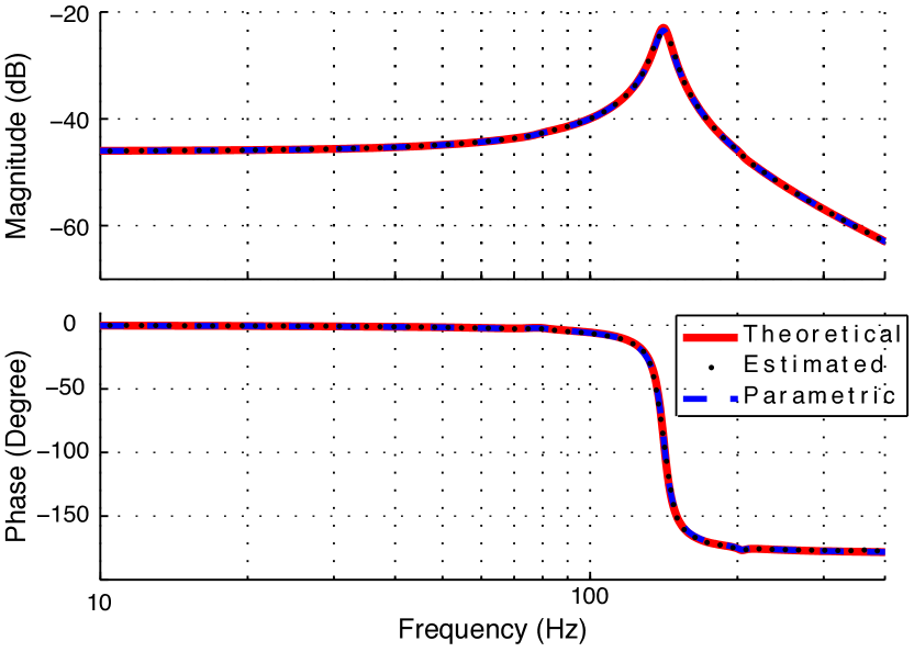
Figure 3: Estimation results for the fundamental harmonic.

The resulting output is then subtracted from the numerically measured limit cycle to obtain error trajectories $\xi_{1}$ for vertical position. The input signal and $\xi_{1}$ are then used as in Section III-C to estimate harmonic transfer functions for our system. Since our theoretical computations showed that responses beyond the third harmonic were very small, we only consider the fundamental harmonic and three harmonics on both sides for our experiments.

Fig. 3 illustrates the estimation performance of our algorithm for the magnitude and phase of the fundamental harmonic. Both graphs show that the application of the identification algorithm in [14] works well even for nonlinear periodic systems with hybrid dynamics.

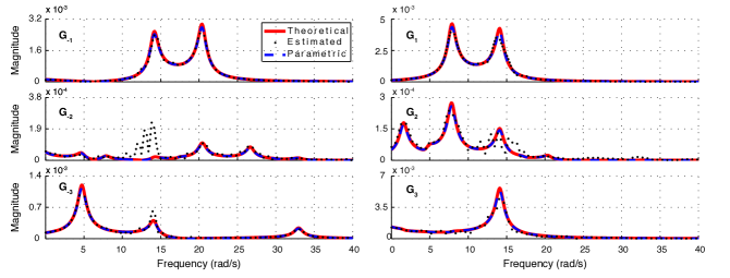
Figure 4: Estimation results for the higher order harmonics.

We also show our identification results for three harmonics in both the negative and positive sides in Fig. 4. Even though magnitudes for the harmonic transfer functions are small compared to the fundamental, the identification algorithm can provide accurate estimates for these transfer functions except in some narrow regions of $G_{-2}$ and $G_{2}$. The identification algorithm could not correctly estimate these two harmonics around $12-15$ (rad/s). One possible reason for this discrepancy is the presence of strong responses in all harmonics around the same frequency except $G_{-2}$ and $G_{2}$, resulting in the inability of the identification algorithm to distinguish between the contributions from each harmonic absent knowledge of the internal system dynamics. Alternatively, these discrepancies may also be a result of the fact that hybrid transitions are not strictly time periodic (rather, they are state-dependent) which likely has effects on different frequencies and harmonics. We plan on investigating these issues further in the future.

For a comparative analysis, we also present results from a parametric identification in order to show that further corrections on estimation results from a non-parametric method are possible. To this end, we fit the system parameters $k$ and $c$ in (25) by comparing root mean square error between theoretically computed and estimated harmonic transfer functions $G_{0}$, $G_{-1}$ and $G_{1}$. We truncate the system response after the first harmonic in order to discard erroneous regions in higher harmonics. The resulting estimates were $\hat{k}=200$ for the spring constant and $\hat{c}=2.12$ for the damping coefficient, which closely coincide with the parameters used to generate the input–output data. As such, harmonic transfer functions obtained from parametric identification were found to closely match those obtained from theoretical computations as seen in Fig. 4.

Motivated by these identification results, we plan to extend our work to the identification of the Spring-Loaded Inverted Pendulum (SLIP) model [3] and its extensions, widely used as models of locomotory behaviors in the literature. Our future goal is to apply our system identification methods to our physical monopod robot platform and to compare the identification performances with our previously verified analytical model [11].

V Conclusion

In this paper, we presented a system identification strategy to estimate input–output transfer functions for a simple hybrid spring mass damper system as a step towards data-driven models for legged locomotion. We first showed that a class of hybrid locomotion models can be approximated with a piecewise constant LTP systems in close proximity to their asymptotically stable limit-cycle. Our analysis and identification framework is based on the concept of harmonic transfer functions [24].

We first observed that the hybrid system dynamics associated with this model exhibits piecewise LTI behavior around its periodic orbit. We then represented this behavior as a purely time periodic system around the limit cycle in order to utilize system identification techniques applicable to Linear Time Periodic systems.

In order to provide a basis for comparison, we computed analytic expressions for harmonic transfer functions associated with the LTP approximation to our simplified hybrid model. In our theoretical analysis, we considered the system’s response up to the $10^{th}$ harmonic. We observed that there were no meaningful responses on both positive and negative sides after the third harmonic. Therefore, we decided to truncate the system response after the third harmonic during our identification studies.

We then performed systematic simulation studies and identified the harmonic transfer functions of the same model without knowledge of its internal dynamics. We used an input signal consisting of successive chirp signals, with phases evenly distributed across the system’s period, to obtain a full characterization of system dynamics for our frequency range of interest. Our studies showed that LTP system identification techniques can successfully be used to identify the transfer functions of nonlinear periodic models with hybrid system dynamics.

References

- [1] P. J. Holmes, R. J. Full, D. E. Koditschek, and J. Guckenheimer, “The dynamics of legged locomotion: Models, analyses, and challenges,” SIAM Rev, vol. 48, no. 2, pp. 207–304, 2006.
- [2] R. J. Full and D. E. Koditschek, “Templates and anchors: neuromechanical hypotheses of legged locomotion on land,” J Exp Biol, vol. 202, no. 23, pp. 3325–3332, 1999.
- [3] W. J. Schwind, “Spring loaded inverted pendulum running: A plant model,” PhD Thesis, University of Michigan, Ann Arbor, MI, USA, 1998.
- [4] R. J. Full and M. S. Tu, “Mechanics of a rapid running insect: two-, four-, and six-legged locomotion,” J Exp Biol, vol. 156, pp. 215–231, 1991.
- [5] P. Holmes, “Poincaré, celestial mechanics, dynamical-systems theory and “chaos”.” Physics Reports, vol. 193, pp. 137–163, September 1990.
- [6] W. J. Schwind and D. E. Koditschek, “Approximating the stance map of a 2 dof monoped runner,” Journal of Nonlinear Science, vol. 10, no. 5, pp. 533–588, July 2000.
- [7] H. Geyer, A. Seyfarth, and R. Blickhan, “Spring-mass running: Simple approximate solution and application to gait stability,” Journal of Theoretical Biology, vol. 232, no. 3, pp. 315–328, February 2005.
- [8] U. Saranli, O. Arslan, M. M. Ankaralı, and Ö. Morgül, “Approximate analytic solutions to non-symmetric stance trajectories of the passive spring-loaded inverted pendulum with damping,” Nonlinear Dynamics, vol. 62, pp. 729–742, December 2010.
- [9] M. M. Ankarali and U. Saranli, “Stride-to-stride energy regulation for robust self-stability of a torque-actuated dissipative spring-mass hopper,” Chaos: An Interdisciplinary Journal of Nonlinear Science, vol. 20, no. 3, p. 033121, September 2010.
- [10] I. Uyanik, U. Saranli, and Ö. Morgül, “Adaptive control of a spring-mass hopper,” in IEEE International Conference on Robotics and Automation (ICRA), 2011, pp. 2138–2143.
- [11] I. Uyanik, Ö. Morgül, and U. Saranli, “Experimental validation of a feed-forward predictor for the spring-loaded inverted pendulum template,” IEEE Transactions on Robotics, 2015.
- [12] U. Saranli, M. Buehler, and D. E. Koditschek, “RHex: A simple and highly mobile robot,” International Journal of Robotics Research, vol. 20, no. 7, pp. 616–631, July 2001.
- [13] N. W. Wereley, “Analysis and control of linear periodically time varying systems,” Ph.D., Massachusetts Institute of Technology, Dept. of Aeronautics and Astronautics, 1991.
- [14] A. Siddiqi, “Identification of the harmonic transfer functions of a helicopter rotor,” M.Sc., Massachusetts Institute of Technology, Dept. of Aeronautics and Astronautics, 2001.
- [15] S. Hwang, “Frequency domain system identification of helicopter rotor dynamics incorporating models with time periodic coefficients,” Ph.D., Graduate School of the University of Maryland at College Park, 1997.
- [16] M. W. Sracic and M. S. Allen, “Method for identifying models of nonlinear systems using linear time periodic approximations,” Mechanical Systems and Signal Processing, vol. 25, no. 7, pp. 2705 – 2721, 2011.
- [17] M. M. Ankarali and N. J. Cowan, “System identification of rhythmic hybrid dynamical systems via discrete time harmonic transfer functions,” in Proc IEEE Int Conf on Decision and Control, Los Angeles, CA, USA, December 2014.
- [18] K. C. Galloway, G. C. Haynes, B. D. Ilhan, A. M. Johnson, R. Knopf, G. Lynch, B. Plotnick, M. White, and D. E. Koditschek, “X-rhex: A highly mobile hexapedal robot for sensorimotor tasks,” University of Pennsylvania, Tech. Rep., 2010.
- [19] U. Saranli, A. Avci, and M. C. Öztürk, “A modular real-time fieldbus architecture for mobile robotic platforms,” IEEE Transactions on Instrumentation and Measurement, vol. 60, no. 3, pp. 916–927, 2011.
- [20] S. Revzen and J. M. Guckenheimer, “Estimating the phase of synchronized oscillators,” Physical Review, vol. 78, no. 5, p. 051907, November 2008.
- [21] J. Guckenheimer and S. Johnson, “Planar hybrid systems,” in Hybrid systems II. Springer, 1995, pp. 202–225.
- [22] A. Wu and H. Geyer, “The 3-d spring–mass model reveals a time-based deadbeat control for highly robust running and steering in uncertain environments,” IEEE Transactions on Robotics, 2013.
- [23] A. Leonhard, “The describing function method applied for the investigation of parametric oscillations,” in Proceedings of the 2nd IFAC World Conference, 1963, pp. 21–28.
- [24] N. Wereley and S. Hall, “Frequency response of linear time periodic systems,” in Proceedings of the 29th IEEE Conference on Decision and Control, 1990, pp. 3650–3655 vol.6.
- [25] E. Möllerstedt, “Dynamic analysis of harmonics in electrical systems,” Ph.D., Lund Institute of Technology, Department of Automatic Control, 2000.
- [26] G. Piovan and K. Byl, “Two-element control for the active slip model,” in IEEE International Conference on Robotics and Automation (ICRA), May 2013, pp. 5656–5662.
- [27] G. Secer and U. Saranli, “Control of monopedal running through tunable damping,” in Signal Processing and Communications Applications Conference (SIU), 2013 21st, April 2013, pp. 1–4.
- [28] I. Uyanik, “Adaptive control of a one-legged hopping robot through dynamically embedded spring-loaded inverted pendulum template,” M.Sc., Bilkent Univ., Ankara, Turkey, August 2011.