Sketch and Validate for Big Data Clustering

Abstract

In response to the need for learning tools tuned to big data analytics, the present paper introduces a framework for efficient clustering of huge sets of (possibly high-dimensional) data. Building on random sampling and consensus (RANSAC) ideas pursued earlier in a different (computer vision) context for robust regression, a suite of novel dimensionality- and set-reduction algorithms is developed. The advocated sketch-and-validate (SkeVa) family includes two algorithms that rely on $K$-means clustering per iteration on reduced number of dimensions and/or feature vectors: The first operates in a batch fashion, while the second sequential one offers computational efficiency and suitability with streaming modes of operation. For clustering even nonlinearly separable vectors, the SkeVa family offers also a member based on user-selected kernel functions. Further trading off performance for reduced complexity, a fourth member of the SkeVa family is based on a divergence criterion for selecting proper minimal subsets of feature variables and vectors, thus bypassing the need for $K$-means clustering per iteration. Extensive numerical tests on synthetic and real data sets highlight the potential of the proposed algorithms, and demonstrate their competitive performance relative to state-of-the-art random projection alternatives.

Keywords. Clustering, high-dimensional data, variable selection, feature vector selection, sketching, validation, $K$-means.

1 Introduction

As huge amounts of data are collected perpetually from communication, imaging, and mobile devices, medical and e-commerce platforms as well as social-networking sites, this is undoubtedly an era of data deluge [10]. Such “big data” however, come with “big challenges.” The sheer volume and dimensionality of data make it often impossible to run analytics and traditional inference methods using stand-alone processors, e.g., [3, 17]. Consequently, “workhorse” learning tools have to be re-examined in the face of today’s high-cardinality sets possibly comprising high-dimensional data.

Clustering (a.k.a. unsupervised classification) refers to categorizing into groups unlabeled data encountered in the widespread applications of mining, compression, and learning tasks [4]. Among numerous clustering algorithms, $K$-means is the most prominent one thanks to its simplicity [4]. It thrives on “tight” groups of feature vectors, data points or objects that can be separated via (hyper)planes. Its scope is further broadened by the so-termed probabilistic and kernel $K$-means, with an instantiation of the latter being equivalent to spectral clustering – the popular tool for graph-partitioning that can cope even with nonlinearly separable data [12].

A key question with regards to clustering data sets of cardinality $N$ containing $D$-dimensional vectors with $N$ and/or $D$ huge, is: How can one select the most “informative” vectors and/or dimensions so as to reduce their number for efficient computations, yet retain as much of their cluster-discrimination capability? This paper develops such an approach for big data $K$-means clustering. Albeit distinct, the inspiration comes from random sampling and consensus (RANSAC) methods, which were introduced for outlier-resilient regression tasks encountered in computer vision [14, 30, 25, 35, 29, 8].

Feature selection is a rich topic [15] explored extensively from various angles, including pattern recognition, source coding and information theory, (combinatorial) optimization [33, 31], and neural networks [6]. Unfortunately, most available selection schemes do not scale well with the number of features $D$, particularly in the big data regime where $D$ is massive. Recent approaches to dimensionality reduction and clustering include subspace clustering, where minimization problems requiring singular value decompositions (SVDs) are solved per iteration to determine in parallel a low-dimensional latent space and corresponding sparse coefficients for efficient clustering [26]. Low-dimensional subspace representations are also pursued in the context of kernel $K$-means [7, Alg. 2], where either an SVD on a sub-sampled kernel matrix, or, the solution of a quadratic optimization task is required per iteration to cluster efficiently large-scale data.

Randomized schemes select features with non-uniform probabilities that depend on the so-termed “leverage scores” of the data matrix [19, 20]. Unfortunately, their complexity is loaded by the leverage scores computation, which, similar to [26], requires SVD computations – a cumbersome (if not impossible) task when $D\gg$ and/or $N\gg$. Recent computationally efficient alternatives for feature selection and clustering rely on random projections (RPs) [19, 20, 9, 5]. Specifically for RP-based clustering [5], the data matrix is left multiplied by a data-agnostic (fat) $d\times D$ RP matrix to reduce its dimension ($d\ll D$); see also [18] where RPs are employed to accelerate the kernel $K$-means algorithm. Clustering is performed afterwards on the reduced $d$-dimensional vectors. With its universality and quantifiable performance granted, this “one-RP-matrix-fits-all” approach is not as flexible to adapt to the data-specific attributes (e.g., low rank) that is typically present in big data.

This paper’s approach aspires to not only account for structure, but also offer a gamut of novel randomized algorithms trading off complexity for clustering performance by developing a family of what we term sketching and validation (SkeVa) algorithms. The SkeVa family includes two algorithms based on efficient intermediate $K$-means clustering steps. The first is a batch method, while the second is sequential thus offering computational efficiency and suitability for streaming modes of operation. The third member of the SkeVa family is kernel-based and enables big data clustering of even nonlinearly separable data sets. Finally, the fourth one bypasses the need for intermediate $K$-means clustering thus trading off performance for complexity. Extensive numerical validations on synthetic and real data-sets highlight the potential of the proposed methods, and demonstrate their competitive performance on clustering massive populations of high-dimensional data vs. state-of-the-art RP alternatives.

Notation. Boldface uppercase (lowercase) letters indicate matrices (column vectors). Calligraphic uppercase letters denote sets ($\varnothing$ stands for the empty set), and $|\mathcal{A}|$ expresses the cardinality of $\mathcal{A}$. Operators $\|\cdot\|_{2}$ and $\|\cdot\|_{1}$ stand for the $\ell_{2}$- and $\ell_{1}$-norm of a vector, respectively, while $(\cdot)^{\top}$ denotes transposition and $\bm{1}$ the all-one vector.

2 Preliminaries

Consider the $D\times N$ data matrix $\bm{X}:=[\bm{x}_{1},\ldots,\bm{x}_{N}]$ with $D$ and/or $N$ being potentially massive. Data $\{\bm{x}_{n}\}_{n=1}^{N}$ belong to a known number of $K$ clusters ($K\ll N$). Each cluster $\mathcal{C}_{k}$ is represented by its centroid $\bm{c}_{k}$ that can be e.g., the (sample) mean of the vectors in $\mathcal{C}_{k}$. Accordingly, each datum can be modeled as $\bm{x}_{n}=\bm{C}\bm{\pi}_{n}+\bm{v}_{n}$, where $\bm{C}:=[\bm{c}_{1},\ldots,\bm{c}_{K}]$; the sparse $K\times 1$ vector $\bm{\pi}_{n}$ comprises the data-cluster association entries satisfying $\sum_{k=1}^{K}[\bm{\pi}_{n}]_{k}=1$, where $[\bm{\pi}_{n}]_{k}\in(0,1]$ when $\bm{x}_{n}\in\mathcal{C}_{k}$, while $[\bm{\pi}_{n}]_{k}=0$, otherwise; and the noise $\bm{v}_{n}$ captures $\bm{x}_{n}$’s deviation from the corresponding centroid(s).

For hard clustering, the said associations are binary ($[\bm{\pi}_{n}]_{k}\in\{0,1\}$), and in the celebrated hard $K$-means algorithm they are identified based on the Euclidean ($\ell_{2}$) distance between $\bm{x}_{n}$ and its closest centroid. Specifically, given $K$ and $\{\bm{x}_{n}\}_{n=1}^{N}$, per iteration $i=1,2,\ldots$, the $K$-means algorithm iteratively updates data-cluster associations and cluster centroids as follows; see e.g., [4].

[$$i n=1,\ldots,N$$-a] Update data-cluster associations: For ,

$$\bm{x}_{n}\in\mathcal{C}_{k}[i] \Leftrightarrow k\in\operatorname*{argmin}_{k^{\prime}\in\{1,\ldots,K\}}\left\lVert\bm{x}_{n}-\bm{c}_{k^{\prime}}[i]\right\rVert_{2}^{2}\;.$$ (1b)

[$$i k=1,\ldots,K$$-b] Update cluster centroids: For ,

$$\bm{c}_{k}[i+1] \in\operatorname*{argmin}_{\bm{c}\in\mathbb{R}^{D}}\sum_{\bm{x}_{n}\in\mathcal{C}_{k}[i]}\lVert\bm{x}_{n}-\bm{c}\rVert_{2}^{2}$$

$$=\frac{1}{\bigl{|}\mathcal{C}_{k}[i]\bigr{|}}\sum\nolimits_{\bm{x}_{n}\in\mathcal{C}_{k}[i]}\bm{x}_{n}\;.$$ (1c)

Although there may be multiple assignments solving (1b), each $\bm{x}_{n}$ is assigned to a single cluster. To initialize (1b), one can randomly pick $\{\bm{c}_{k}[1]\}_{k=1}^{K}$ from $\{\bm{x}_{n}\}_{n=1}^{N}$. The iterative algorithm (1) solves a challenging NP-hard problem, and albeit its success, $K$-means guarantees convergence only to a local minimum at complexity $\mathcal{O}(NDKI)$, with $I$ denoting the number of iterations needed for convergence, which depends on initialization [4, § 9.1].

Remark 1.

As (1b) and (1c) minimize an $\ell_{2}$-norm squared, hard $K$-means is sensitive to outliers. Variants exhibiting robustness to outliers adopt non-Euclidean distances (a.k.a. dissimilarity metrics) $\delta$, such as the $\ell_{1}$-norm. In addition, candidate “centroids” can be selected per iteration from the data themselves; that is, $\bm{c}\in\mathcal{C}_{k}[i]$ in (1c). Notwithstanding for this so-termed $K$-medoids algorithm, one just needs the distances $\{\delta(\bm{x}_{n},\bm{x}_{n^{\prime}})\}$ to carry out the minimizations in (1b) and (1c). The latter in turn allows $\{\bm{x}_{n}\}_{n=1}^{N}$ to even represent non-vectorial objects (a.k.a. qualitative data), so long as the aforementioned (non-)Euclidean distances can become available otherwise; e.g., in the form of correlations [4, § 9.1].

Besides various distances and centroid options, hard $K$-means in (1) can be generalized in three additional directions: (i) Using nonlinear functions $\varphi:\mathbb{R}^{D}\to\mathcal{H}$, with $\mathcal{H}$ being a potentially infinite-dimensional space, data $\{\bm{x}_{n}\}$ can be transformed to $\{\varphi(\bm{x}_{n})\}$, where clustering can be facilitated (cf. Sec. 3.3); (ii) via non-binary $\bm{\pi}_{n}\in[0,1]^{K}$, soft clustering can allow for multiple associations per datum, and thus for a probabilistic assignment of data to clusters; and (iii) additional constraints (e.g., sparsity) can be incorporated in the $[\bm{\pi}_{n}]_{k}$ coefficients through appropriate regularizers $\rho(\bm{\pi})$.

All these generalizations can be unified by replacing (1) per iteration $i=1,2,\ldots$, with

[$$i n=1,\ldots,N$$-a] Update data-cluster associations: ,

$$\bm{\pi}_{n}[i]\in\operatorname*{argmin}_{\begin{subarray}{c}\bm{\pi}\in[0,1]^{K};\\ \bm{1}^{\top}\bm{\pi}=1\end{subarray}}\delta\left(\varphi(\bm{x}_{n}),\sum_{k=1}^{K}\pi_{k}\bm{c}_{k}[i]\right)+\rho(\bm{\pi})\,.$$ (2b)

[$$i$$-b] Update cluster centroids:

$$\{\bm{c}_{k}[i+1]\}_{k=1}^{K}\in\smashoperator[l]{\operatorname*{argmin}_{\{\bm{c}_{k}\}_{k=1}^{K}\subset\mathcal{H}}^{}}\sum_{n=1}^{N}\delta\left(\varphi(\bm{x}_{n}),\sum_{k=1}^{K}\bigl{[}\bm{\pi}_{n}[i]\bigr{]}_{k}\bm{c}_{k}\right)\,.$$ (2c)

In Sec. 3.3, function $\varphi$ will be implicitly used to map nonlinearly separable data $\{\bm{x}_{n}\}_{n=1}^{N}$ to linearly separable (possibly infinite dimensional) data $\{\varphi(\bm{x}_{n})\}_{n=1}^{N}$, whose distances can be obtained through a pre-selected (so-termed kernel) function $\kappa$ [4, Chap. 6]. The regularizer $\rho(\bm{\pi})$ can enforce prior knowledge on the data-cluster association vectors.

To confirm that indeed (1) is subsumed by (2), let $\varphi(\bm{x}_{n})=\bm{x}_{n}$; choose $\delta$ as the squared Euclidean distance in $\mathbb{R}^{D}$; and set $\rho(\bm{\pi})=0$, if $\bm{\pi}\in\mathcal{E}_{K}:=\{\bm{e}_{k}\}_{k=1}^{K}$, whereas $\rho(\bm{\pi})=+\infty$ otherwise, with $\bm{e}_{k}$ being the $k$th $K$-dimensional canonical vector. Then (2b) becomes $\bm{\pi}_{n}[i]\in\operatorname*{argmin}_{\bm{\pi}\in\{0,1\}^{K};\,\bm{1}^{\top}\bm{\pi}=1}\lVert\bm{x}_{n}-\sum_{k}\pi_{k}\bm{c}_{k}[i]\rVert_{2}^{2}$, which further simplifies to the minimum distance rule of (1b). Moreover, it can be readily verified that (2c) $\{\bm{c}_{k}[i+1]\}_{k=1}^{K}\in\operatorname*{argmin}_{\{\bm{c}_{k}\}_{k=1}^{K}}\sum_{n}\lVert\bm{x}_{n}-\sum_{k}[\bm{\pi}_{n}[i]]_{k}\bm{c}_{k}\rVert_{2}^{2}$ separates across $k$s to yield the centroid of (1c) per cluster.

To recognize how (2) captures also soft clustering, consider that cluster $\mathcal{C}_{k}$ is selected with probability $\pi_{k}:=\operatorname{Pr}(\mathcal{C}_{k})$, and its data are drawn from a probability density function (pdf) $p$ parameterized by $\bm{\theta}_{k}$; i.e., $\bm{x}|\mathcal{C}_{k}\sim p(\bm{x};\bm{\theta}_{k})$. If $p$ is Gaussian, then $\bm{\theta}_{k}$ denotes its mean $\bm{\mu}_{k}$ and covariance matrix $\bm{\Sigma}_{k}$. With $\bm{\theta}:=[\bm{\theta}_{1}^{\top},\ldots,\bm{\theta}_{K}^{\top}]^{\top}$ and allowing for multiple cluster associations, the likelihood per datum is given by the mixture pdf: $p(\bm{x};\bm{\pi},\bm{\theta})=\sum_{k=1}^{K}\pi_{k}p(\bm{x};\bm{\theta}_{k})$, which for independently drawn data yields the joint log-likelihood ($\bm{\Pi}:=[\bm{\pi}_{1},\ldots,\bm{\pi}_{N}]$)

$$\ln\,p(\bm{X};\bm{\Pi},\bm{\theta})=\sum_{n=1}^{N}\ln\biggl{(}\sum_{k=1}^{K}[\bm{\pi}_{n}]_{k}p(\bm{x}_{n};\bm{\theta}_{k})\biggr{)}\,.$$ (3)

If $\varphi(\bm{x}_{n}):=\bm{x}_{n}$, $\bm{c}_{k}:=p(\bm{x}_{n};\bm{\theta}_{k})$, and $\delta(\bm{x}_{n},\sum_{k}\pi_{k}c_{k}):=-\ln(\sum_{k}[\bm{\pi}_{n}]_{k}p(\bm{x}_{n};\bm{\theta}_{k}))$ in (2), then soft $K$-means iterations (2b) and (2c) maximize (3) with respect to (w.r.t.) $\bm{\Pi}$ and $\bm{\theta}$. An alternative popular maximizer of the likelihood in (3) is the expectation-maximization algorithm; see e.g., [4, § 9.3].

If the number of clusters $K$ is unknown, it can also be estimated by regularizing the log-likelihood in (3) with terms penalizing complexity as in e.g., minimum description length criteria [4].

Although hard $K$-means is the clustering module common to all numerical tests in Sec. V, the novel big data algorithms of Secs. III and IV apply to all schemes subsumed by (2).

3 The SkeVa Family

Our novel algorithms based on random sketching and validation are introduced in this section. Relative to existing clustering schemes, their merits are pronounced when $D$ and/or $N$ take prohibitively large values for the unified iterations (2b) and (2c) to remain computationally feasible.

3.1 Batch algorithm

For specificity, the SkeVa K-means algorithm will be developed first for $D\gg$, followed by its variant for $N\gg$.

Using a repeated trial-and-error approach, SkeVa K-means discovers a few dimensions (features) that yield high-accuracy clustering. The key idea is that upon sketching a small enough subset of dimensions (trial or sketching phase), a hypotheses test can be formed by augmenting the original subset with a second small subset (up to $d$ affordable dimensions) to validate whether the first subset nominally represents the full $D$-dimensional data (error phase). Such a trial-and-error procedure is repeated for a number $R_{\max}$ of realizations, after which the features that have achieved the “best” clustering accuracy results are those determining the final clusters on the whole set of dimensions.

Starting with the trial-phase per realization $r$, $\check{d}$ dimensions (rows) of $\bm{X}$ are randomly drawn (uniformly) to obtain $\check{\bm{X}}^{(r)}:=[\check{\bm{x}}_{1}^{(r)},\ldots,\check{\bm{x}}_{N}^{(r)}]\in\mathbb{R}^{\check{d}\times N}$. With $\check{d}$ small enough, $K$-means is run on $\check{\bm{X}}^{(r)}$ to obtain clusters $\{\check{\mathcal{C}}_{k}^{(r)}\}_{k=1}^{K}$ and corresponding centroids $\{\check{\bm{c}}_{k}^{(r)}\}_{k=1}^{K}$ [cf. (1b) and (1c)]. These sketching and clustering steps comprise the (random) sketching phase.

Moving on to the error-phase of the procedure, the quality of the $\check{d}$-dimensional clustering is assessed next using what we term validation phase. This starts by re-drawing $\check{d}^{\prime}$-dimensional data $\{\check{\bm{x}}_{n}^{(r^{\prime})}\}_{n=1}^{N}$ $(\check{d}^{\prime}\ll D-\check{d})$, generally different from those selected in draw $r$. Associating each $\check{\bm{x}}_{n}^{(r^{\prime})}$ with the cluster $\check{\bm{x}}_{n}^{(r)}$ belongs to, the centroids corresponding to the extra $\check{d}^{\prime}$ dimensions are formed as [cf. (1c)]

$$\check{\bm{c}}_{k}^{(r^{\prime})}=\frac{1}{\bigl{\lvert}\check{\mathcal{C}}_{k}^{(r)}\bigr{\rvert}}\sum_{\check{\bm{x}}_{n}^{(r)}\in\check{\mathcal{C}}_{k}^{(r)}}\check{\bm{x}}_{n}^{(r^{\prime})}\,.$$ (4)

Let $\bar{\bm{x}}_{n}^{(r)}:=[\check{\bm{x}}_{n}^{(r)}{}^{\top},\check{\bm{x}}_{n}^{(r^{\prime})}{}^{\top}]^{\top}$ and $\bar{\bm{c}}_{k}^{(r)}:=[\check{\bm{c}}_{k}^{(r)}{}^{\top},\check{\bm{c}}_{k}^{(r^{\prime})}{}^{\top}]^{\top}$ denote respectively the concatenated data and centroids from draws $r$ and $r^{\prime}$, and likewise for the data and centroid matrices $\bar{\bm{X}}^{(r)}$ and $\bar{\bm{C}}^{(r)}$. Measuring distances $\{\delta(\bar{\bm{x}}_{n}^{(r)},\bar{\bm{c}}_{k}^{(r)})\}$ and using again the minimum distance rule data-cluster associations and clusters $\{\bar{\mathcal{C}}_{k}^{(r)}\}_{k=1}^{K}$ are obtained for the “augmented data.” If per datum $\bm{x}_{n}$ the data-cluster association in the space of $\check{d}$ dimensions coincides with that in the space of $d:=\check{d}+\check{d}^{\prime}$ dimensions, then $\bm{x}_{n}$ is in the validation set (VS) $\mathcal{V}_{D}^{(r)}$; that is,

$$\mathcal{V}_{D}^{(r)}:=\left\{\bm{x}_{n}\Bigm{|}\check{\bm{x}}_{n}^{(r)}\in\check{\mathcal{C}}_{k_{1}}^{(r)},\bar{\bm{x}}_{n}^{(r)}\in\bar{\mathcal{C}}_{k_{2}}^{(r)},\ \text{and}\ k_{1}=k_{2}\right\}\,.$$ (5)

Quality of clustering per draw is then assessed using a monotonically increasing rank function $f$ of the set $\mathcal{V}_{D}^{(r)}$. Based on this function, a $\check{d}$-dimensional trial $r_{1}$ is preferred over another $\check{d}$-dimensional trial $r_{2}$ if $f(\mathcal{V}_{D}^{(r_{1})})>f(\mathcal{V}_{D}^{(r_{2})})$.

The sketching and validation phases are repeated for a prescribed number of realizations $R_{\max}$. At last, the $\check{d}$-dimensional sketching $r_{*}:=\operatorname*{argmax}_{r\in\{1,\ldots,R_{\max}\}}f(\mathcal{V}_{D}^{(r)})$ yields the final clusters, namely $\{\check{\mathcal{C}}_{k}^{(r_{*})}\}_{k=1}^{K}$; see Alg. 1.

1:Data $\bm{X}$; number of clusters $K$; reduced dimensions $\check{d}$ and $\check{d}^{\prime}$ for the sketching and validation phases, respectively; ranking function $f$; number of realizations (draws) $R_{\max}$.

2:Data-cluster associations on $\bm{X}$.

3:for $r=1$ to $R_{\max}$ do

4:    Randomly sample $\check{d}\ll D$ rows of $\bm{X}$ to obtain $\check{\bm{X}}^{(r)}$.

5:    Run $K$-means on $\check{\bm{X}}^{(r)}$; obtain clusters $\{\check{\mathcal{C}}_{k}^{(r)}\}_{k=1}^{K}$ and centroids $\{\check{\bm{c}}_{k}^{(r)}\}_{k=1}^{K}$ [cf. (1)].

6:    Randomly sample $\check{d}^{\prime}\ll D$ rows of $\bm{X}$ (other than those in step 4) to obtain $\check{\bm{X}}^{(r^{\prime})}$.

7:    Per cluster $k$, form $\bar{\bm{c}}_{k}^{(r)}:=[\check{\bm{c}}_{k}^{(r)}{}^{\top},\check{\bm{c}}_{k}^{(r^{\prime})}{}^{\top}]^{\top}$.

8:    Associate $\{\bar{\bm{x}}_{n}^{(r)}\}_{n=1}^{N}$ to closest $\{\bar{\bm{c}}_{k}^{(r)}\}_{k=1}^{K}$.

9:    Identify validation set $\mathcal{V}_{D}^{(r)}$ [cf. (5)].

10:end for

11:$r_{*}:=\arg\max_{r\in\{1,\ldots,R_{\max}\}}f(\mathcal{V}_{D}^{(r)})$.

12:Associate data to clusters on $\bm{X}$ as in $\{\check{\mathcal{C}}_{k}^{(r_{*})}\}_{k=1}^{K}$.

Algorithm 1 Batch SkeVa K-means

With regards to selecting $f$, a straightforward choice is the VS cardinality, that is $f(\mathcal{V}_{D}^{(r)}):=\lvert\mathcal{V}_{D}^{(r)}\rvert$, which can be thought as the empirical probability of correct clustering. Alternatively, a measure of cluster separability, used extensively in pattern recognition, is Fisher’s discriminant ratio [4], which in the present context becomes

$$\text{FDR}^{(r)}:=\sum_{k_{1}=1}^{K}\sum_{\begin{subarray}{c}k_{2}=1;\\ k_{2}\neq k_{1}\end{subarray}}^{K}\frac{\left\lVert\bar{\bm{c}}_{k_{1}}^{(r)}-\bar{\bm{c}}_{k_{2}}^{(r)}\right\rVert_{2}^{2}}{\bigl{(}\bar{\sigma}_{k_{1}}^{(r)}\bigr{)}^{2}+\bigl{(}\bar{\sigma}_{k_{2}}^{(r)}\bigr{)}^{2}}$$ (6)

where $(\bar{\sigma}_{k}^{(r)})^{2}$ is the unbiased sample variance of cluster $k$:

$$\bigl{(}\bar{\sigma}_{k}^{(r)}\bigl{)}^{2}:=\frac{1}{\lvert\check{\mathcal{C}}_{k}^{(r)}\rvert-1}\sum_{\check{\bm{x}}_{n}\in\check{\mathcal{C}}_{k}^{(r)}}\left\lVert\bar{\bm{x}}_{n}^{(r)}-\bar{\bm{c}}_{k}^{(r)}\right\rVert_{2}^{2}\;.$$ (7)

The larger the $\text{FDR}^{(r)}$, the more separable clusters are. Obtaining $\text{FDR}^{(r)}$ is computationally light since distances in (7) have been calculated during the validation phase of the algorithm. The only additional burden is computing the numerator in (6) in $\mathcal{O}[(\check{d}+\check{d}^{\prime})K^{2}]$ complexity. Based on FDR, a second choice for $f$ is

$$f(\mathcal{V}_{D}^{(r)})=\bigl{\lvert}\mathcal{V}_{D}^{(r)}\bigr{\rvert}\exp\left(-\frac{1}{\text{FDR}^{(r)}}\right)\,.$$

Instead of $\text{FDR}^{(r)}$, the exponent is $-1/\text{FDR}^{(r)}$ to avoid pathological cases where $\text{FDR}^{(r)}$ approaches $+\infty$, e.g., when all points in a cluster are very concentrated so that $(\bar{{\sigma}}_{k}^{(r)})^{2}\approx 0$.

Alg. 1 incurs overall complexity $\mathcal{O}(NKR_{\max}\check{d}I)$, where $I$ is an upper bound on the number of iterations needed for $K$-means to converge in step 5, plus $\mathcal{O}(NKR_{\max}\check{d}^{\prime})$ required in step 8 of Alg. 1. Parameters $\check{d}$, $\check{d}^{\prime}$, and $R_{\max}$ are selected depending on the available computational resources; $(\check{d},\check{d}^{\prime})$ should be such that running the computations of Alg. 1 on $(\check{d}+\check{d}^{\prime})$-dimensional vectors can be affordable by the processing unit used. A probabilistic argument for choosing $R_{\max}$ can be determined as elaborated next.

Remark 2.

Using parameters that can be obtained in practice, it is possible to relate the number of random draws $R_{\max}$ with the reliability of SkeVa-based clustering, along the lines of analyzing RANSAC [14].

To this end, let $p$ denote the probability of having out of $R$ SkeVa realizations at least one “good draw” of $\check{d}$ “informative” dimensions, meaning one for which $K$-means yields data-cluster associations close to those found by $K$-means on the full set of $D$ dimensions. Parameter $p$ is a function of the underlying cluster characteristics. It can be selected by the user and reflects one’s level of SkeVa-based big data clustering reliability, e.g., $p:=0.95$. The probability of having all “bad draws” after $R$ SkeVa repetitions is clearly $1-p$. Moreover, let $q$ denote the probability that a randomly drawn row of $\bm{X}$ is “informative.” In other words, $q$ quantifies prior information on the number of rows (out of $D$) that carry high discriminative information for $K$-means. For instance, $q$ can be practically defined by the leverage scores of $\bm{X}$, which typically rank the importance of rows of $\bm{X}$ in large-scale data analytics [5, 20]. An estimate of the leverage scores across the rows of $\bm{X}$ expresses $q$ as the percentage of informative rows. Alternatively, if $\bm{x}_{n_{j}}=\bm{m}_{k}+\bm{\Sigma}_{k}^{1/2}\bm{v}_{n_{j}}$ is the data generation mechanism per cluster $k$, with $\bm{v}_{n_{j}}\sim\mathcal{N}(\bm{0},\bm{I}_{D})$, then the $i$th entry of $\bm{x}_{n_{j}}$ is $\bm{e}_{i}^{\top}\bm{x}_{n_{j}}\sim\mathcal{N}(\bm{e}_{i}^{\top}\bm{m}_{k},[\bm{\Sigma}_{k}]_{ii})$. Thus, rows of $\bm{X}$ are realizations of a Gaussian $1\times N$ random vector. If these rows are clustered in $K^{\prime}$ groups, $q$ can capture the probability of having an “informative” row located within a confidence region around its associated centroid that contains a high percentage $\alpha\in(0,1)$ of its pdf mass. Per SkeVa realization, the probability of drawing $\check{d}$ “non-informative” rows can be approximated by $(1-q)^{\check{d}}$. Due to the independence of SkeVa realizations, $1-p=(1-q)^{{\check{d}}R}$, which implies that $R\simeq\log(1-p)/[\check{d}\log(1-q)]$. Clearly, as $R$ increases there is (a growing) nonzero probability that the correct clusters will be revealed. On the other hand, it must be acknowledged that if $R$ is not sufficient, clustering performance will suffer commensurately.

It is interesting to note that as in [14], $R$ only depends implicitly on $D$, since $q$ is a percentage, and does not depend on the validation metric or pertinent thresholds and bounds.

3.2 Sequential algorithm

1:Data $\bm{X}$; number of clusters $K$; reduced dimensions $\check{d}$ and $\check{d}^{\prime}$ of reduced dimensions for the sketching and validation phases, respectively; ranking function $f$; number of realizations (draws) $R_{\max}$.

2:Data-cluster associations on $\bm{X}$.

3:for $r=1$ to $R_{\max}$ do

4:    Randomly sample $\check{d}\ll D$ rows of $\bm{X}$ to obtain $\check{\bm{X}}^{(r)}$.

5:    Run $K$-means on $\check{\bm{X}}^{(r)}$ to obtain clusters $\{\check{\mathcal{C}}_{k}^{(r)}\}_{k=1}^{K}$ and centroids $\{\check{\bm{c}}_{k}^{(r)}\}_{k=1}^{K}$.

6:    Initialize the auxiliary set of dimensions $\mathcal{A}=\emptyset$.

7:   for $j=1$ to $\check{d}^{\prime}$ do

8:       Randomly sample $1$ dimension of $\bm{X}$ (other than those in step 4 and in $\mathcal{A}$) to obtain row $\check{\mathbf{x}}^{(r^{\prime})}$ of $\bm{X}$.

9:       Include sampled dimension in $\mathcal{A}$.

10:       Form $\{\bar{\bm{c}}_{k}^{(r)}:=[\check{\bm{c}}_{k}^{(r)}{}^{\top},\check{c}_{k}^{(r^{\prime})}]^{\top}\}_{k=1}^{K}$ as in Alg. 1.

11:       Associate $\{\bar{\bm{x}}_{n}^{(r)}\}_{n=1}^{N}$ to closest $\{\bar{\bm{c}}_{k}^{(r)}\}_{k=1}^{K}$.

12:       Identify validation set $\mathcal{V}_{D}^{(r)}$ [cf. (5)].

13:      if $f(\mathcal{V}_{D}^{(r)})<f_{\max}^{(r)}$ or $|\nabla f(\mathcal{V}_{D}^{(r)})|\leq\epsilon$ then

14:          Go to step 4.

15:      end if

16:   end for

17:    $f_{\max}^{(r+1)}=f(\mathcal{V}_{D}^{(r)})$.

18:    $r_{*}=r$.

19:end for

20:Data-cluster associations on $\bm{X}$ according to $\{\check{\mathcal{C}}_{k}^{(r_{*})}\}_{k=1}^{K}$.

Algorithm 2 Sequential (Se)SkeVa K-means.

Drawing a batch of $\check{d}^{\prime}$ features (rows of $\bm{X}$) during the validation phase of Alg. 1 to assess the discriminating ability of the features drawn in the sketching phase may be computationally, especially if $\check{d}^{\prime}$ is relatively large. The computation of all distances $\{\delta(\bar{\bm{x}}_{n}^{(r)},\bar{\bm{c}}_{k}^{(r)})\}$ in step 8 of Alg. 1 can be prohibitive if $\check{d}^{\prime}$ becomes large. This motivates a sequential augmentation of dimensions, where features are added one at a time, and computations are performed on only a single row of $\bm{X}$ per feature augmentation, till the upper-bound $\check{d}^{\prime}$ is reached. Apparently, such an approach adds flexibility and effects computational savings since sequential augmentation of dimensions does not need to be carried out till $\check{d}^{\prime}$ is reached, but it may be terminated early on if a prescribed criterion is met. These considerations prompted the development of Alg. 2.

The sketching phase of Alg. 2 remains the same as in Alg. 1. In the validation phase, and for each dimension in the additional $\check{d}^{\prime}$ ones, $\{\check{\bm{c}}_{k}^{(r^{\prime})}\}_{k=1}^{K}$ are obtained as in Alg. 1 [cf. (4)], and likewise for $\mathcal{V}_{D}^{(r)}$. If $f(\mathcal{V}_{D}^{(r)})$ is smaller than the current maximum value $f_{\max}^{(r)}$ in memory, the $\check{d}$-dimensional clustering $\{\check{\mathcal{C}}_{k}^{(r)}\}$ is discarded, and a new draw is taken. This can be seen as a “bail-out” test, to reject possibly “bad clusterings” in time, without having to perform the augmentation using all $\check{d}^{\prime}$ dimensions.

Experiments corroborate that it is not necessary to augment all $D-\check{d}$ dimensions (cf. Fig. 1), but using a small subset of them provides satisfactory accuracy while reducing complexity. An alternative route is to stop augmentation once the “gradient” of $f$, meaning finite differences across augmented dimensions, drops below a prescribed $\epsilon>0$; that is, $|\nabla f(\mathcal{V}_{D}^{(r)})|\leq\epsilon$. The sequential approach is summarized in Alg. 2, and has complexity strictly smaller than $\mathcal{O}[NKR_{\max}(\check{d}I+\check{d}^{\prime})]$.

Remark 3.

Using $N$ in the place of $D$ whenever $D\ll N$, or equivalently, replacing $\bm{X}\in\mathbb{R}^{D\times N}$ with $\bm{X}^{\top}$, both the batch and sequential schemes developed for $D\gg$ can be implemented verbatim for $N\gg$. This variant of SkeVa K-means will be detailed in the next subsection for nonlinearly separable clusters.

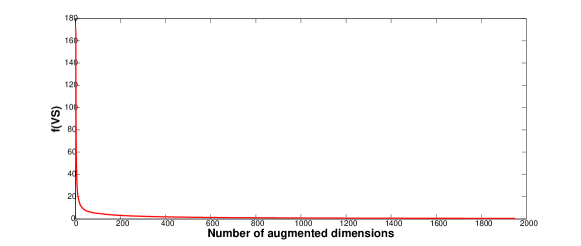
Figure 1: $f(\mathcal{V}_{D}^{(r)})$ vs. the number of augmented dimensions $\check{d}^{\prime}$ for a synthetic data-set, with $D=2,000,N=1,000$, $\check{d}=50$, and full-rank data-model (cf. Secs. 3.2 and 5).

3.3 Big data kernel clustering

A prominent approach to clustering or classifying nonlinearly separable data is through kernels; see e.g., [4]. Vectors $\{\bm{x}_{n}\}_{n=1}^{N}$ are mapped to $\{\varphi(\bm{x}_{n})\}_{n=1}^{N}$ that live in a higher (possibly infinite-) dimensional space $\mathcal{H}$, where inner products defining distances in $\mathcal{H}$, using the induced norm $\lVert\>\cdot\>\rVert_{\mathcal{H}}:=\langle\cdot\mathop{}|\mathop{}\cdot\rangle_{\mathcal{H}}^{1/2}$, are given by a pre-selected (reproducing) kernel function $\kappa$; that is, $\langle\varphi(\bm{x}_{n})\mathop{}|\mathop{}\varphi(\bm{x}_{n^{\prime}})\rangle_{\mathcal{H}}=\kappa(\bm{x}_{n},\bm{x}_{n^{\prime}})$ [4]. An example of such a kernel is the Gaussian one: $\kappa_{\bm{\Sigma}}(\bm{x}_{n},\bm{x}):=\exp[-(\bm{x}-\bm{x}_{n})^{\top}\bm{\Sigma}^{-1}(\bm{x}-\bm{x}_{n})/2]/[(2\pi)^{D/2}(\det\bm{\Sigma})^{1/2}]$.

For simplicity in exposition, our novel kernel-based (Ke)SkeVa K-means approach to big data clustering will be developed for the hard $K$-means. Extensions to kernel-based soft SkeVa K-means follow naturally, and are outlined in Appendix A. Similar to (1), the kernel-based hard $K$-means proceeds as follows. For $i\in\{1,2,\ldots,I\}$,

[$$i n=1,\ldots,N$$-a] Update data-cluster associations: For ,

$$\bm{x}_{n}\in\mathcal{C}_{k}[i] \Leftrightarrow k\in\operatorname*{argmin}_{k^{\prime}\in\{1,\ldots,K\}}\left\lVert\varphi(\bm{x}_{n})-\bm{c}_{k^{\prime}}[i]\right\rVert_{\mathcal{H}}^{2}$$ (8b)

[$$i k=1,\ldots,K$$-b] Update cluster centroids: For ,

$$\bm{c}_{k}[i+1] \in\operatorname*{argmin}_{\bm{c}\in\mathcal{H}}\sum\nolimits_{\bm{x}_{n}\in\mathcal{C}_{k}[i]}\lVert\varphi(\bm{x}_{n})-\bm{c}\rVert_{\mathcal{H}}^{2}$$

$$=\frac{1}{\bigl{|}\mathcal{C}_{k}[i]\bigr{|}}\sum\nolimits_{\bm{x}_{n}\in\mathcal{C}_{k}[i]}\varphi(\bm{x}_{n})$$ (8c)

where Euclidean norms $\lVert\>\cdot\>\rVert_{2}$ in the standard form of $K$-means have been replaced by $\lVert\>\cdot\>\rVert_{\mathcal{H}}$. As the potentially infinite-size $\{\bm{c}_{k}[i+1]\}_{k=1}^{K}$ cannot be stored in memory, step (8c) is implicit. In fact, only $\kappa$ and the data-cluster associations suffice to run (8). To illustrate this, substitute $\{\bm{c}_{k}[i+1]\}_{k=1}^{K}$ from (8c) into (8b) to write

$$\left\lVert\varphi(\bm{x}_{n})-\frac{1}{\bigl{|}\mathcal{C}_{k^{\prime}}[i+1]\bigr{|}}\sum\nolimits_{\bm{x}^{\prime}_{n}\in\mathcal{C}_{k^{\prime}}[i+1]}\varphi(\bm{x}^{\prime}_{n})\right\rVert_{\mathcal{H}}^{2}$$

$$=\langle\varphi(\bm{x}_{n})\mathop{}|\mathop{}\varphi(\bm{x}_{n})\rangle_{\mathcal{H}}$$ (9)

$$\hphantom{=\ }-\frac{2}{\bigl{|}\mathcal{C}_{k^{\prime}}[i+1]\bigr{|}}\sum_{\bm{x}^{\prime}_{n}\in\mathcal{C}_{k^{\prime}}[i+1]}\langle\varphi(\bm{x}_{n})\mathop{}|\mathop{}\varphi(\bm{x}^{\prime}_{n})\rangle_{\mathcal{H}}$$

$$\hphantom{=\ }+\frac{1}{\bigl{|}\mathcal{C}_{k^{\prime}}[i+1]\bigr{|}^{2}}\smashoperator[r]{\sum_{(\bm{x}^{\prime}_{n},\bm{x}^{\prime\prime}_{n})\in(\mathcal{C}_{k^{\prime}}[i+1])^{2}}^{}}\langle\varphi(\bm{x}^{\prime}_{n})\mathop{}|\mathop{}\varphi(\bm{x}^{\prime\prime}_{n})\rangle_{\mathcal{H}}$$

$$=\kappa(\bm{x}_{n},\bm{x}_{n})-\frac{2}{\bigl{|}\mathcal{C}_{k^{\prime}}[i+1]\bigr{|}}\smashoperator[r]{\sum_{\bm{x}^{\prime}_{n}\in\mathcal{C}_{k^{\prime}}[i+1]}^{}}\kappa(\bm{x}_{n},\bm{x}^{\prime}_{n})$$

$$\hphantom{=\ }+\frac{1}{\bigl{|}\mathcal{C}_{k^{\prime}}[i+1]\bigr{|}^{2}}\smashoperator[r]{\sum_{(\bm{x}^{\prime}_{n},\bm{x}^{\prime\prime}_{n})\in(\mathcal{C}_{k^{\prime}}[i+1])^{2}}^{}}\kappa(\bm{x}^{\prime}_{n},\bm{x}^{\prime\prime}_{n})\,.$$ (10)

Having established that distances involved in SkeVa K-means are expressible in terms of the chosen kernel $\kappa$, the resulting iterative scheme is listed as Alg. 3. After randomly selecting an affordable subset $\check{\bm{X}}^{(r)}$, comprising $\check{\nu}$ columns of $\bm{X}$ per realization $r$, and similar to the trial-and-error step in line 5 of Alg. 1, the (kernel) $K$-means of (8) is applied to $\check{\bm{X}}^{(r)}$. The validation phase of KeSkeVa K-means is initialized in line 6, where a second subset $\check{\bm{X}}^{(r^{\prime})}$ comprising $\check{\nu}^{\prime}$ columns from $\bm{X}\setminus\check{\bm{X}}^{(r)}$. The distances between data $\{\varphi(\bm{x}_{n}^{(r^{\prime})})\}$ and centroids $\{\check{\bm{c}}_{k}^{(r)}\}$ involved in step 7 of Alg. 3 are also obtained through kernel evaluations [cf. (10)]. This KeSkeVa that operates on the number of data-points rather than dimensions follows along the line of RANSAC [14] but with two major differences: (i) Instead of robust parameter regression, it is tailored for big data clustering; and (ii) rather than consensus it deals with affordably small validation sets across possibly huge data-sets.

During the validation phase, clusters $\check{\mathcal{C}}_{k}^{(r^{\prime})}$ are specified according to $\bm{x}_{n}^{(r^{\prime})}\in\check{\mathcal{C}}_{k}^{(r^{\prime})}\Leftrightarrow k\in\operatorname*{argmin}_{k^{\prime}\in\{1,\ldots,K\}}\lVert\varphi(\bm{x}_{n}^{(r^{\prime})})-\check{\bm{c}}_{k^{\prime}}^{(r)}\rVert^{2}_{\mathcal{H}}$. Gathering all information from draws $(r,r^{\prime})$, the augmented clusters $\bar{\mathcal{C}}_{k}^{(r)}:=\check{\mathcal{C}}_{k}^{(r)}\cup\check{\mathcal{C}}_{k}^{(r^{\prime})}$ (step 7 of Alg. 3) lead to centroids

$$\bar{\bm{c}}_{k}^{(r)}:=\frac{1}{\bigl{\lvert}\bar{\mathcal{C}}_{k}^{(r)}\bigr{\rvert}}\smashoperator[r]{\sum_{\bm{x}_{n}\in\bar{\mathcal{C}}_{k}^{(r)}}^{}}\varphi(\bm{x}_{n})\,.$$ (11)

Given the “implicit centroids” obtained as in (11), data $\bm{X}^{(r)}$ are mapped to clusters $\{\bar{\mathcal{C}}_{k}^{(r)}\}$ which are different from $\check{\mathcal{C}}_{k}^{(r)}$. To assess this difference, the distance between $\varphi(\bm{x}_{n}^{(r)}$ and $\bar{\bm{c}}_{k}^{(r)}$ is computed, and columns of $\bm{X}^{(r)}$ are re-grouped in clusters $\{\check{\bar{\mathcal{C}}}_{k}^{(r)}\}_{k=1}^{K}$ as

$$\bm{x}_{n}^{(r)}\in\check{\bar{\mathcal{C}}}_{k}^{(r)}\Leftrightarrow k\in\operatorname*{argmin}_{k^{\prime}\in\{1,\ldots,K\}}\left\lVert\varphi\bigl{(}\bm{x}_{n}^{(r)}\bigr{)}-\bar{\bm{c}}_{k^{\prime}}^{(r)}\right\rVert^{2}_{\mathcal{H}}\,.$$ (12)

Recall that distances are again obtained through kernel evaluations [cf. (10)].

The process of generating clusters and centroids in KeSkeVa K-means can be summarized as follows: (i) Group randomly drawn data $\bm{X}^{(r)}$ into clusters $\check{\mathcal{C}}_{k}^{(r)}$ with centroids $\check{\bm{c}}_{k}^{(r)}$; (ii) draw additional data-points, augment clusters $\bar{\mathcal{C}}_{k}^{(r)}$, and compute new centroids $\bar{\bm{c}}_{k}^{(r)}$; (iii) given $\bar{\bm{c}}_{k}^{(r)}$, find clusters $\check{\bar{\mathcal{C}}}_{k}^{(r)}$ as in (12). Since $\check{\bm{c}}_{k}^{(r)}\neq\bar{\bm{c}}_{k}^{(r)}$ in general, data belonging to $\check{\mathcal{C}}_{k}^{(r)}$ do not necessarily belong to $\check{\bar{\mathcal{C}}}_{k}^{(r)}$, and vice versa; while data common to $\check{\bar{\mathcal{C}}}_{k}^{(r)}$ and $\check{\mathcal{C}}_{k}^{(r)}$, that is data that have not changed “cluster membership” during the validation phase, comprise the validation set

$$\mathcal{V}_{N}^{(r)}:=\Bigl{\{}\bm{x}_{n}^{(r)}\in\check{\bm{X}}^{(r)}\Bigm{|}\exists k\ \text{s.t.}\ \bm{x}_{n}^{(r)}\in\Bigl{(}\check{\mathcal{C}}_{k}^{(r)}\cap\check{\bar{\mathcal{C}}}_{k}^{(r)}\Bigr{)}\Bigr{\}}\,.$$ (13)

Among $R_{\max}$ realizations, trial $r_{*}$ with the highest cardinality $|\mathcal{V}_{N}^{(r_{*})}\rvert$ is identified in Alg. 3, and data are finally associated with clusters $\{\check{\mathcal{C}}_{k}^{(r_{*})}\}_{k=1}^{K}$. The overall complexity of Alg. 3 is $\mathcal{O}(DKR_{\max}\check{\nu}^{2}I)$ in step 5, when $\{\kappa(\bm{x}_{n},\bm{x}_{n^{\prime}})\}_{n,n^{\prime}=1}^{N}$ are not stored in memory and kernel evaluations have to be performed for all employed data per realization, plus $\mathcal{O}(DR_{\max}\check{\nu}\check{\nu}^{\prime})$ in step 7. If $\{\kappa(\bm{x}_{n},\bm{x}_{n^{\prime}})\}_{n,n^{\prime}=1}^{N}$ are stored in memory, then Alg. 3 incurs complexity $\mathcal{O}(KR_{\max}\check{\nu}^{2}I+R_{\max}\check{\nu}\check{\nu}^{\prime})$, which is quadratic only in the small cardinality $\check{\nu}$.

1:Data $\bm{X}$; number of clusters $K$; number $\check{\nu}$ and $\check{\nu}^{\prime}$ of data during sketching and validation phase, respectively; number of realizations $R_{\max}$.

2:Data-cluster associations on $\bm{X}$.

3:for $r=1$ to $R_{\max}$ do

4:    Randomly sample $\check{\nu}\ll N$ columns of $\bm{X}$ to obtain $\check{\bm{X}}^{(r)}$.

5:    Apply $K$-means [cf. (20) and (2)] on $\{\varphi(\bm{x}_{n}^{(r)})\}_{n=1}^{\check{\nu}}$; obtain clusters $\{\check{\mathcal{C}}_{k}^{(r)}\}_{k=1}^{K}$ and centroids $\{\check{\bm{c}}_{k}^{(r)}\}_{k=1}^{K}$.

6:    Randomly select $\check{\nu}^{\prime}\ll N$ columns of $\bm{X}$, other than those of step 4, to obtain $\check{\bm{X}}^{(r^{\prime})}$.

7:    Associate $\{\varphi(\bm{x}_{n}^{(r^{\prime})})\}_{n=1}^{\check{\nu}^{\prime}}$ to the closest centroids $\{\check{\bm{c}}_{k}^{(r)}\}_{k=1}^{K}$; obtain clusters $\{\bar{\mathcal{C}}_{k}^{(r)}\}_{k=1}^{K}$ and centroids $\{\bar{\bm{c}}_{k}^{(r)}\}_{k=1}^{K}$ [cf. (11)].

8:    Obtain clusters $\{\check{\bar{\mathcal{C}}}_{k}^{(r)}\}$ on $\check{\bm{X}}^{(r)}$ according to (12).

9:    Identify the validation set $\mathcal{V}_{N}^{(r)}$.

10:end for

11:$r_{*}=\arg\min_{r\in\{1,\ldots,R_{\max}\}}\lvert\mathcal{V}_{N}^{(r)}\rvert$.

12: Associate $\{\varphi(\bm{x}_{n})\}_{n=1}^{N}$ according to the closest centroids obtained from clusters $\{\check{\mathcal{C}}_{k}^{(r_{*})}\}_{k=1}^{K}$.

Algorithm 3 Kernel (Ke)SkeVa K-means

One remark is now in order.

Remark 4.

Similar to all kernel-based approaches, a critical issue is selecting the proper kernel – more a matter of art and prior information about the data. Nonetheless, practical so-termed multi-kernel approaches adopt a dictionary of kernels from which one or a few are selected to run $K$-means on [23]. It will be interesting to investigate whether such multi-kernel approaches can be adapted to our SkeVa-based operation to alleviate the dependence on a single kernel function.

4 Divergence-Based SkeVa

A limitation of Algs. 1 and 2 is the trial-and-error strategy which requires clustering per random draw of samples. This section introduces a method to surmount such a need and select a small number of data or dimensions on which only a single clustering step is applied at the last stage of the algorithm. As the “quality” per draw is assessed without clustering, this approach trades off accuracy for reduced complexity.

4.1 Large-scale data sets

First, the case where random draws are performed on the $N$ data will be examined, followed by draws across the $D$ dimensions. Any randomly drawn data from $\{\bm{x}_{n}\}_{n=1}^{N}$ will be assumed centered around their sample mean.

Since intermediate clustering will not be applied to assess the quality of a random draw, a metric is needed to quantify how well the randomly drawn samples represent clusters. To this end, motivated by the pdf mixture model [cf. (3)], consider the following pdf estimate formed using the randomly selected data

$$\check{p}^{(r)}(\bm{x}):=\frac{1}{\check{\nu}}\sum_{n=1}^{\check{\nu}}\kappa\bigl{(}\bm{x}_{n}^{(r)},\bm{x}\bigr{)}$$ (14)

where $\kappa$ stands for a user-defined kernel function, parameterized by $\bm{x}_{n}^{(r)}$, and satisfying
$\int\kappa(\bm{x}_{n}^{(r)},\bm{x})d\bm{x}=1$ for the estimate in (14) to qualify as a pdf. Here, the Gaussian kernel $\kappa_{\bm{\Sigma}}(\bm{x}_{n}^{(r)},\bm{x}):=\exp[-(\bm{x}-\bm{x}_{n}^{(r)})^{\top}\bm{\Sigma}^{-1}(\bm{x}-\bm{x}_{n}^{(r)})/2]/[(2\pi)^{D/2}(\det\bm{\Sigma})^{1/2}]$ is considered with $\bm{\Sigma}:=\sigma^{2}\bm{I}_{D}$.

Having linked random samples with pdf estimates, the assessment whether a draw represents well the whole population $\{\bm{x}_{n}\}_{n=1}^{N}$ translates to how successful this draw is in estimating the actual data pdf via (14). A random sample where all selected data form a single cluster is clearly not a good representative of $\{\bm{x}_{n}\}_{n=1}^{N}$. For example, if the selected points are gathered around $\bm{0}$ (recall that drawn data are centered around their sample mean), then the resulting pdf estimate (14) will resemble the uni-modal (thick) dashed curve in Fig. 2. Such a pdf estimate is a poor representative of the whole data-set, and clustering on that small population of data should be avoided. On the contrary, random draws yielding the multi-modal (thick) solid curve in Fig. 2 should be highly rated as potential candidates for clustering. As a first step toward assessing draws is a metric quantifying how “far” the pdf $\check{p}^{(r)}$ is from $\check{p}^{(0)}(\bm{x}):=\kappa(\bm{0},\bm{x})$.

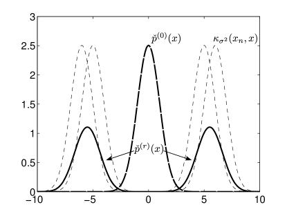
Figure 2: Examples of pdf mixtures fitted to data-points. Reference pdf estimate is the uni-modal thick dashed curve; the larger the divergence from this estimate, the larger the probability of producing meaningful clustering.

Among candidate metrics of “distance” between pdfs, the Cauchy-Schwarz divergence [27] is chosen here:

$$\Delta_{\text{CS}}\bigl{(}\check{p}^{(r)}{\mathop{}\|\mathop{}}\check{p}^{(r^{\prime})}\bigr{)}:=-\log\frac{\left(\int\check{p}^{(r)}(\bm{x})\check{p}^{(r^{\prime})}(\bm{x})d\bm{x}\right)^{2}}{\int[\check{p}^{(r)}(\bm{x})]^{2}d\bm{x}\int[\check{p}^{(r^{\prime})}(\bm{x})]^{2}d\bm{x}}\,.$$

The reason for choosing $\Delta_{\text{CS}}$ over other popular divergences, such as the Kullback-Leibler one, is the ease of obtaining pdf estimates via (14). Specifically, the numerator in $\Delta_{\text{CS}}$ can be expressed as [cf. (14)]

$$\int \check{p}^{(r)}(\bm{x})\check{p}^{(r^{\prime})}(\bm{x})d\bm{x}$$

$$=\frac{1}{\check{\nu}\check{\nu}^{\prime}}\sum_{n=1}^{\check{\nu}}\sum_{n^{\prime}=1}^{\check{\nu}^{\prime}}\int\kappa\bigl{(}\bm{x}_{n}^{(r)},\bm{x}\bigr{)}\kappa\bigl{(}\bm{x}_{n^{\prime}}^{(r^{\prime})},\bm{x}\bigr{)}d\bm{x}\,.$$ (15)

The right-hand-side of (15) is simplified further if the chosen kernel is the Gaussian one. As the convolution of Gaussian pdfs is also Gaussian, it is not hard to verify that

$$\int\kappa_{\bm{\Sigma}}\bigl{(}\bm{x}_{n}^{(r)},\bm{x}\bigr{)}\kappa_{\bm{\Sigma}}\bigl{(}\bm{x}_{n^{\prime}}^{(r^{\prime})},\bm{x}\bigr{)}d\bm{x}=\kappa_{2\bm{\Sigma}}\bigl{(}\bm{x}_{n}^{(r)},\bm{x}_{n^{\prime}}^{(r^{\prime})}\bigr{)}$$

for which (15) becomes

$$\int\check{p}^{(r)}(\bm{x})\check{p}^{(r^{\prime})}(\bm{x})d\bm{x}=\frac{1}{\check{\nu}\check{\nu}^{\prime}}\bm{1}^{\top}\bm{K}_{2\bm{\Sigma}}^{(r,r^{\prime})}\bm{1}$$

where the $\check{\nu}\times\check{\nu}^{\prime}$ matrix $\bm{K}_{2\bm{\Sigma}}^{(r,r^{\prime})}$ has $(n,n^{\prime})$th entry $[\bm{K}_{2\bm{\Sigma}}^{(r,r^{\prime})}]_{nn^{\prime}}:=\kappa_{2\bm{\Sigma}}(\bm{x}_{n}^{(r)},\bm{x}_{n^{\prime}}^{(r^{\prime})})$. It thus follows that

$$\Delta_{\text{CS}}\bigl{(}\check{p}^{(r)}{\mathop{}\|\mathop{}}\check{p}^{(r^{\prime})}\bigr{)}= -2\log\left(\frac{1}{\check{\nu}\check{\nu}^{\prime}}\bm{1}^{\top}\bm{K}_{2\bm{\Sigma}}^{(r,r^{\prime})}\bm{1}\right)$$

$$+\log\left(\frac{1}{\check{\nu}^{2}}\bm{1}^{\top}\bm{K}_{2\bm{\Sigma}}^{(r,r)}\bm{1}\right)$$

$$+\log\left(\frac{1}{\check{\nu}^{\prime}{}^{2}}\bm{1}^{\top}\bm{K}_{2\bm{\Sigma}}^{(r^{\prime},r^{\prime})}\bm{1}\right)\,.$$ (16)

Notice that when $r^{\prime}$ is simply $\{\bm{0}\}$, the last summand in (16) becomes $\log\kappa_{2\bm{\Sigma}}(\bm{0},\bm{0})=-D(\log 2\pi)/2-(\log\det 2\bm{\Sigma})/2$.

1:Data $\bm{X}$; number of clusters $K$; number $\check{\nu}$ and $\check{\nu}^{\prime}$ of points for sketching and validation phases, respectively; number of realizations $R_{\max}$; $\Delta_{\max}=0$, $\Delta^{\prime}_{\min}=+\infty$.

2:Data-cluster associations.

3:for $r=1$ to $R_{\max}$ do

4:    Let $\check{\bm{X}}^{(r)}$ denote $\check{\nu}$ randomly selected points after centered around their sample mean.

5:   if $\Delta_{\text{CS}}(\check{p}^{(r)}{\mathop{}\|\mathop{}}\check{p}^{(0)})>\Delta_{\max}$ then

6:       Let $\check{\bm{X}}^{(r^{\prime})}$ denote $\check{\nu}^{\prime}$ randomly selected points, other than those in step 4, after centered around their sample mean.

7:       $\bar{\bm{X}}^{(r)}:=[\check{\bm{X}}^{(r)},\check{\bm{X}}^{(r^{\prime})}]$.

8:      if $\Delta_{\text{CS}}(\bar{p}^{(r)}{\mathop{}\|\mathop{}}\check{p}^{(r^{\prime})})<\Delta^{\prime}_{\min}$ then

9:         $\Delta^{\prime}_{\min}:=\Delta_{\text{CS}}(\bar{p}^{(r)}{\mathop{}\|\mathop{}}\check{p}^{(r^{\prime})})$.

10:         $\Delta_{\max}:=\Delta_{\text{CS}}(\check{p}^{(r)}{\mathop{}\|\mathop{}}\check{p}^{(0)})$.

11:         $r_{*}:=r$.

12:      end if

13:   end if

14:end for

15:Perform $K$-means on $\check{\bm{X}}^{(r_{*})}$ and associate $\bm{X}$ to clusters obtained by $K$-means on $\check{\bm{X}}^{(r_{*})}$.

Algorithm 4 Divergence (Di)SkeVa K-means on $N$.

The metric in (16) is computed per draw of the so-termed divergence-based DiSkeVa K-means summarized in Alg. 4. A number $R_{\max}$ of realizations are attempted to discover a “good” draw $r_{*}$ of data, to which clustering is finally performed. Line 5 in Alg. 4 checks whether the randomly selected subset yield via (14) a pdf $\check{p}^{(r)}$ that differs enough from the “singular” pdf $\check{p}^{(0)}=\kappa_{\bm{\Sigma}}(\bm{0},\cdot)$. If the divergence exceeds $\Delta_{\max}$, realization $r$ will be further explored, otherwise $r+1$ is drawn. Notice that threshold $\Delta_{\max}$ is adaptively defined and takes, according to line 10, the maximum recorded value from realization $r=0$ till the current one.

If $\check{p}^{(r)}$ passes the first check of being far from $\check{p}^{(0)}$, lines 6 to 12 implement the second step of consenting whether $r$ is indeed a “good” realization. To this end, a number of $\check{\nu}^{\prime}$ additional data-points is drawn to form $\bar{\bm{X}}^{(r)}:=[\check{\bm{X}}^{(r)},\check{\bm{X}}^{(r^{\prime})}]$ in line 7. The mixture pdf $\bar{p}^{(r)}$ corresponding to $\bar{\bm{X}}^{(r)}$, should stay as close as possible to $\check{p}^{(r)}$ since reliable pdf estimates should remain approximately invariant as extra data are added. Drastic changes of $\Delta_{\text{CS}}$ before and after augmentation suggests that the draw is likely not to be a good representative of the whole population. Notice here that $\Delta^{\prime}_{\min}$ is also adaptively defined to take the minimum value among all recorded divergences from the start of iterations. Moreover, both updates of $\Delta^{\prime}_{\min}$ and $\Delta_{\max}$ are performed once the candidate draw $r$ has passed through the “check-points” of lines 5 and 8.

In the case where the Gaussian kernel is employed, Alg. 4 has overall complexity $o[DR_{\max}\check{\nu}^{2}+DR_{\max}(\check{\nu}\check{\nu}^{\prime}+\check{\nu}^{\prime}{}^{2})]$, if the kernel matrix $\bm{K}_{2\bm{\Sigma}}$ of all data $\{\bm{x}_{n}\}_{n=1}^{N}$ is not stored in memory and calculations of all kernel sub-matrices in (16) are performed per realization; plus, $\mathcal{O}(D\check{\nu}KI)$ for a single application of $K$-means on the finally selected draw $r_{*}$. If $\bm{K}_{2\bm{\Sigma}}$ is available in memory, then Alg. 4 incurs complexity $o[R_{\max}\check{\nu}^{2}+R_{\max}(\check{\nu}\check{\nu}^{\prime}+\check{\nu}^{\prime}{}^{2})+D\check{\nu}KI]$, that is quadratic only in the small subset sizes.

Remark 5.

Along the lines of Remark 2, let $p$ denote the probability of having out of $R$ SkeVa realizations at least one “good draw” of size $\check{\nu}$, meaning one for which $K$-means yields centroids close to those found with the “full data-set.” Moreover, let $q$ denote the probability of a datum to lie “close” to its associated centroid. For example, $q$ can capture the probability of having a datum located within a confidence region which is centered at its associated centroid and contains a high percentage of its pdf mass. The probability of having all “bad draws” is clearly $1-p$. Assuming that data are drawn independently, the probability of having one draw contain only data located “far away” from centroids is $(1-q)^{\check{\nu}}$. Due to the independence of random draws in SkeVa, $1-p=(1-q)^{{\check{\nu}}R}$, which implies that $R\simeq\log(1-p)/[\check{\nu}\log(1-q)]$. Analogous to Remark 2, this argument neither involves $N$ nor it depends on the validation metric or pertinent thresholds and bounds.

4.2 High-dimensional data

Alg. 4 remains operational also when DiSkeVa K-means deals with $D\gg$. Although the proposed scheme can be generalized to cope with both $N\gg$ and $D\gg$, for simplicity of exposition it will be assumed that only $D\gg$. To this end, consider the following pdf estimate $\mathbb{R}^{\check{d}}$:

$$\check{p}^{(r)}(\check{\bm{x}}):=\frac{1}{N}\sum_{n=1}^{N}\kappa\bigl{(}\check{\bm{x}}_{n}^{(r)},\check{\bm{x}}\bigr{)}\,,\quad\forall\check{\bm{x}}\in\mathbb{R}^{\check{d}}$$

where $\check{\bm{x}}_{n}^{(r)}$ denotes a $\check{d}\times 1$ subvector of the $D\times 1$ vector $\bm{x}_{n}$.

The counterpart of Alg. 4 on dimensions is listed as Alg. 5. Although along the lines of Alg. 4, there is a notable difference. In the validation step, where dimensions are increased (cf. line 8) and a pdf estimate is needed for the augmented set of variables. To define divergence between pdfs of different dimensions, vectors have to be zero padded from the $\check{d}$-dimensional $\check{\bm{x}}_{n}^{(r)}$ to the $(\check{d}+\check{d}^{\prime})$-dimensional $\bar{\bm{\chi}}_{n}^{(r)}:=[\check{\bm{x}}_{n}^{(r)}{}^{\top},\bm{0}^{\top}]^{\top}$. Recall here that $\bar{\bm{x}}_{n}^{(r)}:=[\check{\bm{x}}_{n}^{(r)}{}^{\top},\check{\bm{x}}_{n}^{(r^{\prime})}{}^{\top}]^{\top}$. To avoid confusion, pdf mixtures on these zero-padded vectors are given by

$$\bar{q}^{(r)}(\bar{\bm{x}})=\frac{1}{N}\sum_{n=1}^{N}\kappa\bigl{(}\bar{\bm{\chi}}_{n}^{(r)},\bar{\bm{x}}\bigr{)}\,,\quad\forall\bar{\bm{x}}\in\mathbb{R}^{\check{d}+\check{d}^{\prime}}\,.$$ (17)

Similar to Alg. 4, the overall complexity of Alg. 5 is $o[(\check{d}+\check{d}^{\prime})N^{2}R_{\max}]$ for computations in (16), plus $\mathcal{O}(\check{d}NKI)$ for a single application of $K$-means on the finally selected draw $r_{*}$.

1:Data $\bm{X}$; number of clusters $K$; number $\check{d}$ and $\check{d}^{\prime}$ of dimensions for sketching and validation phases, respectively; number of realizations $R_{\max}$; $\Delta_{\max}=0$, $\Delta^{\prime}_{\min}=+\infty$.

2:Data-cluster associations.

3:for $r=1$ to $R_{\max}$ do

4:    Center randomly selected $\check{\bm{X}}^{(r)}$ around their sample mean to obtain $\check{\bm{X}}^{(r)}$.

5:   if $\Delta_{\text{CS}}(\check{p}^{(r)}{\mathop{}\|\mathop{}}\check{p}^{(0)})>\Delta_{\max}$ then

6:       Center randomly selected $\check{\bm{X}}^{(r^{\prime})}$, other than those in step 4, around their sample mean to obtain $\check{\bm{X}}^{(r^{\prime})}$.

7:       Form $\bar{\bm{X}}^{(r)}:=[\check{\bm{X}}^{(r)}{}^{\top},\check{\bm{X}}^{(r^{\prime})}{}^{\top}]^{\top}$.

8:       Form $\bar{\bm{\mathcal{X}}}^{(r)}:=[\check{\bm{X}}^{(r)}{}^{\top},\bm{0}^{\top}]^{\top}$ and estimate pdf mixture $\bar{q}^{(r)}$ [cf. (17)].

9:      if $\Delta_{\text{CS}}(\bar{p}^{(r)}{\mathop{}\|\mathop{}}\bar{q}^{(r)})<\Delta^{\prime}_{\min}$ then

10:         $\Delta^{\prime}_{\min}:=\Delta_{\text{CS}}(\bar{p}^{(r)}{\mathop{}\|\mathop{}}\bar{q}^{(r)})$.

11:         $\Delta_{\max}:=\Delta_{\text{CS}}(\check{p}^{(r)}{\mathop{}\|\mathop{}}\check{p}^{(0)})$.

12:         $r_{*}:=r$.

13:      end if

14:   end if

15:end for

16:Perform $K$-means on $\check{\bm{X}}^{(r_{*})}$ and associate $\bm{X}$ to clusters obtained by $K$-means on $\check{\bm{X}}^{(r_{*})}$.

Algorithm 5 Divergence (Di)SkeVa K-means on $D$.

Remark 6.

If multi-core machines are also available, the validation phases of Algs. 1-5 can be readily parallelized, using recent advances on efficient parallel computing platforms such as MapReduce [11, 13].

5 Numerical Tests

We validated the proposed algorithms on synthetic and real data-sets. Tests involve either large number of data ($N\gg$) and/or large number of dimensions ($D\gg$). The following methods were also tested: (i) The standard hard $K$-means [cf. (1)], run on the full range of $N$ data-points and $D$ dimensions, which is abbreviated in the figures as “full $K$-means”; (ii) the state-of-the-art RP-based feature-extraction scheme [5, Alg. 2], with a Bernoulli-type RP matrix as in [1]; (iii) the randomized feature-selection (RFS) algorithm [5, Alg. 1; $\epsilon=1/3$], a leverage-scores-based scheme; and (iv) the “approximate kernel $K$-means” algorithm [7, Alg. 2], which solves for an “optimal” data-cluster association matrix given a randomly selected subset of the original data-points. For fairness, the naive kernel $K$-means algorithm in [7, Alg. 1] is not tested, because a random draw of data and the application of $K$-means is done only once in [7, Alg. 1]; hence, the attractive attribute of multiple independent draws is not leveraged as in SkeVa. To mitigate initialization-dependent performance, each realization of $K$-means, including also its usage as a module in other competing methods, is run five times with different initialization per run, keeping finally only the data-clusters association that results with the smallest sum of distances of data from the associated centroids.

As figures of merit we adopted the relative clustering accuracy and the execution time (in secs). Relative clustering accuracy is defined as the percentage of points assigned to the correct clusters (empirical probability of correct clustering), relative to that of (kernel) $K$-means on the full data-set. Regarding computational time evaluations, tests in Sec. 5.1 are run using Matlab [22] on a SunFire X$4600$ PC with a $32$-core AMD Opteron $8356$, clocked at $2.3$GHz with $128$GB RAM memory [24], without the use of parallelization, on a single computational thread. Tests in Secs. 5.2, 5.3 and 5.4 are run on an HP ProLiant BL$280$c G$6$ server using $2$ eight-core Sandy Bridge E$5$-$2670$ processor chips ($2.6$GHz) and $128$GB of RAM memory [24]. In the latter tests, algorithms were allowed to exploit MATLAB’s inherent multithread capabilities [21] on the $16$ cores of the server. Moreover, all plotted curves are averages over $50$ Monte Carlo realizations.

To construct synthetic data, $D\times 1$ vectors $\{\bm{x}_{n}\}_{n=1}^{N}$ were generated according to the following model per cluster $k$:

$$\bm{x}_{n_{j}}=\bm{m}_{k}+\bm{\Sigma}_{k}^{1/2}\bm{v}_{n_{j}}\,,\quad j\in\{1,\ldots,{N}/{K}\}$$ (18)

where it is assumed that $N$ is an integer multiple of $K$, $\bm{m}_{k}$ is the $D\times 1$ mean (centroid) of cluster $k$, noise $\bm{v}_{n_{j}}\sim\mathcal{N}(\bm{0},\bm{I}_{D})$ is standardized Gaussian, and $\bm{\Sigma}_{k}$ is the covariance matrix of the data generated for cluster $k$; hence, $\bm{x}_{n_{j}}\sim\mathcal{N}(\bm{m}_{k},\bm{\Sigma}_{k})$. Means $\{\bm{m}_{k}\}_{k=1}^{K}$ are selected uniformly at random from a $D$-dimensional hypercube, as in [5]. To accommodate data-models with limited degrees of freedom, the “rank of data,” controlled by the number of non-zero eigenvalues of $\bm{\Sigma}_{k}$, was used as a tuning parameter. In certain cases, clusters were well separated—a scenario where $K$-means achieves relatively high clustering accuracy. Throughout this section $R_{\max}=10$ except for the tests using the KDDb database [32] for which $R_{\max}=20$.

5.1 Large number of dimensions $(D\gg)$

Tests cases in this subsection have $D\gg N$. Competing methods are the “full $K$-means,” RP [5, Alg. 2], and RFS [5, Alg. 1; $\epsilon=1/3$]. Model (18) was used to generate $N=1,000$ $D$-dimensional vectors for $K=5$ clusters, for several values of $D$, and variable “data-rank.” It can be seen from Figs. 3 and 4 that Algs. 1 (SkeVa K-means) and 2 (SeSkeVa K-means) approach the accuracy of the full $K$-means algorithm as the number of sampled dimensions $d$ increases. As expected, computational time is significantly lower than that of full $K$-means, since the latter operates on all $D$ dimensions. Moreover, SeSkeVa K-means needs more time than RP [5] to achieve the same clustering accuracy (cf. Figs. 3 and 4), since RP utilizes $K$-means as a sub-module only once, after dimensionality-reduction has been effected by left-multiplication of $\bm{X}$ with a (fat) $d\times D$ RP matrix. However, this changes as $D$ grows large. As Fig. 5 demonstrates, whenever $D$ is massive, left-multiplying $\bm{X}$ by the RP $d\times D$ matrix in [5] can become cumbersome, resulting in computational times larger than those of SeSkeVa K-means.

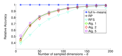
(a) Relative clustering accuracy

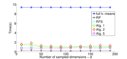
(b) Clustering time (secs)

Figure 3: Synthetic data ($D=2,000$ and full-rank model).

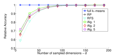
(a) Relative clustering accuracy

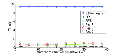
(b) Clustering time (secs)

Figure 4: Synthetic data ($D=2,000$ and rank equal to $500$).

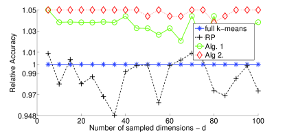
(a) Relative clustering accuracy

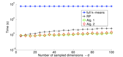
(b) Clustering time (secs)

Figure 5: Synthetic data ($D=500,000$ and rank equal to $1,000$).

Fig. 6 shows results for the real data-set ARCENE [16], which contains mass-spectra of patients diagnosed with cancer, as well as spectra associated with healthy individuals. Clustering involves grouping $100$ ($D=10,000$)-dimensional spectra in two clusters ($K=2$). The number of augmented dimensions for all employed algorithms is $\check{d}^{\prime}=100$. All proposed algorithms approach the performance of RP and full $K$-means, while requiring less time. Alg. 5 is the fastest one at a comparable performance.

Fig. 7 depicts results for the real ORL database of $400$ face-images, from $40$ different subjects ($10$ each) [28, 2]. Images have size $92\times 112$ with $8$-bit grey levels, resulting in $D=10,304$. Only $30$ images ($3$ subjects) were used, and as such the task is to group these images into $K=3$ clusters. As with the ARCENE data, the number of additional dimensions for all proposed algorithms is $\check{d}^{\prime}=100$. Algs. 1, 2, and 5 exhibit similar performance, while requiring much less time than the full $K$-means. Again, Alg. 5 is the fastest one at a comparable performance.

Tests were also performed on a subset of the KDDb 2010 data-set ($K=2$, $D=2,990,384$) [32]. The version of the data-set is the one transformed by the winner of the KDD 2010 Cup (National Taiwan University). In each run $10,000$ data-points were chosen randomly from both classes, and clustering was performed on this subset. The RFS performance is not reported in Fig. 8 as there were issues regarding memory usage due to the required SVD computations. Here, the number of augmented dimensions is $\check{d}^{\prime}=1,000$. All algorithms exhibit performance similar to full $K$-means; however Alg. 1 and Alg. 5 require significantly less time than all competing alternatives.

It should be noted also that the required amount of memory per iteration for Algs. 1 and 2 is at most $\mathcal{O}[N(\check{d}+\check{d}^{\prime})]$, in contrast with the competing algorithms whose memory requirements grow linearly with $D$.

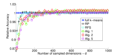
(a) Relative clustering accuracy

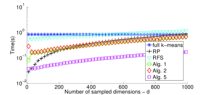
(b) Clustering time (secs)

Figure 6: Simulated performance for real data-set ARCENE.

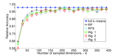
(a) Relative clustering accuracy

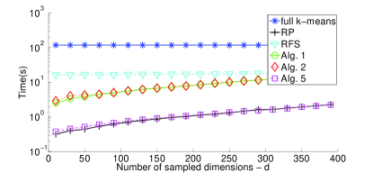
(b) Clustering time (secs)

Figure 7: Simulated performance for real data-set ORL.

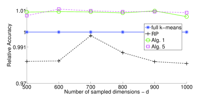
(a) Relative clustering accuracy

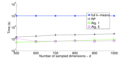
(b) Clustering time (secs)

Figure 8: Simulated performance for real data-set KDDb.

5.2 Large number of points $(N\gg)$

Here we deal with $N\gg D$. Alg. 4 is compared with the “full $K$-means” and the “approximate kernel $K$-means” algorithm [7]. $N=100,000$ vectors with $D=5$ were generated according to (18) for $K=5$ clusters. Although “approximate kernel $K$-means” can accommodate nonlinearly separable clusters by using nonlinear kernel functions, the linear kernel was used here: $\kappa(\bm{x},\bm{y}):=\bm{x}^{\top}\bm{y}$, $\forall\bm{x},\bm{y}$. The Gaussian kernel function $\kappa_{\bm{\Sigma}}$, with $\bm{\Sigma}:=\bm{I}_{D}$, was used in (14). Fig. 9 shows clustering accuracy across the number $\check{\nu}$ of randomly selected data per draw. The number of additional points $\check{\nu}^{\prime}$ is set equal to $100$. As Fig. 9 demonstrates, Alg. 4 approaches the performance of the full $K$-means algorithm, even with $\check{\nu}=100$ sampled data, while requiring markedly lower execution time than both “full” and “approximate kernel $K$-means.”

5.3 Kernel clustering

Nonlinearly separable data are mapped here using a prescribed kernel function to high-dimensional spaces to render them linearly separable. Algs. 3 and 4, with kernel $K$-means applied only at the end, are compared with the “full kernel $K$-means” and the “approximate kernel $K$-means” [7]. Throughout, $\bm{\Sigma}:=5\bm{I}_{D}$ was used in (14). Tests were performed on a subset ($N=35,000$) of the MNIST-$784$ data-set, which contains $28\times 28$ pixel images of handwritten digits grouped in $K=10$ clusters. The kernel used in this case is the sigmoid one $\kappa(\bm{x},\bm{y})=\tanh(\alpha\bm{x}^{\top}\bm{y}+b)$ with parameters $\alpha=0.0045$, $b=0.11$, in accordance to [34]. Both the sigmoid and the Gaussian (for the case of Alg. 4) kernels are considered stored in memory. Fig. 10 depicts the relative clustering accuracy for this data-set and the required time in seconds. It is clear that accuracies of all three algorithms are close and approach the performance of “full kernel $K$-means” as the number of sampled data-points increases. However, the time required by Algs. 3 and 4 is significantly less than the time required by the “full” and “approximate kernel $K$-means.”

5.4 Exploiting multiple computational threads

To showcase the scalability of the proposed algorithms in the presence of multiple computational nodes, the algorithms were run on multiple computational threads. The independent draws $r$ of the proposed algorithms were executed in parallel. Moreover, competing algorithms were allowed to exploit MATLAB’s multithread capabilities, e.g., matrix-matrix multiplications in RP [21]. Figs. 11 and 12 show simulation results for the ARCENE and KDDb data-sets, respectively. Clearly, parallelization of the iterations on the proposed algorithms is beneficial since the algorithms exhibit about an order of magnitude less required time than that of competing methods.

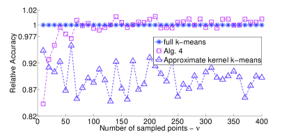
(a) Relative clustering accuracy

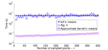
(b) Clustering time (secs)

Figure 9: Synthetic data ($D=5$, $N=100,000$, $K=5$).

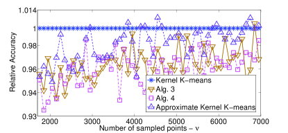
(a) Relative clustering accuracy

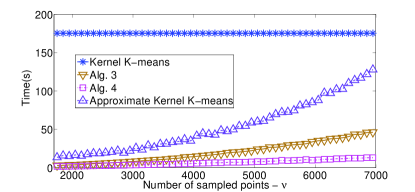
(b) Clustering time (secs)

Figure 10: A subset of the MNIST data-set.

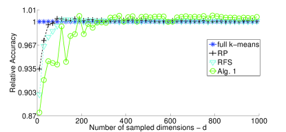
(a) Relative clustering accuracy

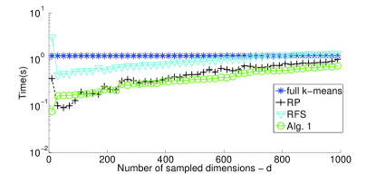
(b) Clustering time (secs)

Figure 11: A subset of the ARCENE data-set with multithreading.

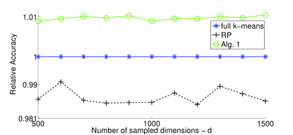
(a) Relative clustering accuracy

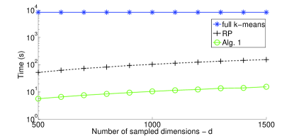
(b) Clustering time (secs)

Figure 12: A subset of the KDDb data-set with multithreading.

6 Conclusions and Future Research

Inspired by RANSAC ideas that have well-appreciated merits for outlier-resilient regression, this paper introduced a novel algorithmic framework for clustering massive numbers of high-dimensional data. Several members of the proposed sketching and validation (SkeVa) family were introduced. The first two members, a batch and a sequential one tailored to streaming modes of operation, required $K$-means clustering in low-dimensional spaces and/or a small number of data-points. To enable clustering of even nonlinearly separable data, a third member of the family leveraged the kernel trick to cluster linearly separable mapped data. A divergence metric was utilized to develop the fourth member of SkeVa K-means that bypasses intermediate $K$-means clustering to trade-off accuracy for reduced complexity. Extensive numerical tests on synthetic and real data-sets demonstrated the competitive performance of SkeVa over state-of-the-art schemes based on random projections. Future research will focus on the rigorous performance analysis of the proposed framework, and on the application of SkeVa to spectral clustering and its MapReduce implementation.

Appendix A Soft Kernel $K$-means

Since this appendix deals with $N\gg$, the clustering schemes of Sec. 2 will be applied here to a reduced number $\check{\nu}$ of $D\times 1$ vectors. Let $\check{\bm{X}}^{(r)}\in\mathbb{R}^{D\times\check{\nu}}$ denote the subset of data obtained by sketching columns of $\bm{X}$. In this context, (2) proceeds as follows. For $i=1,2,\ldots$,

[$$i n=1,\ldots,\check{\nu}$$-a] Update data-cluster associations: For ,

$$\bm{\pi}_{n}[i]\in\operatorname*{argmin}_{\begin{subarray}{c}\bm{\pi}\in[0,1]^{K}\\ \bm{1}^{\top}\bm{\pi}=1\end{subarray}}\delta\left(\varphi\bigl{(}{\bm{x}}_{n}^{(r)}\bigr{)},\sum\nolimits_{k}\pi_{k}\bm{c}_{k}[i]\right)+\rho(\bm{\pi})\,.$$ (19b)

[$$i$$-b] Update cluster centroids:

$$\{\bm{c}_{k}[i+1]\}_{k=1}^{K}\in\smashoperator[l]{\operatorname*{argmin}_{\{\bm{c}_{k}\}\subset\mathcal{H}}^{}}\sum_{n=1}^{\check{\nu}}\delta\left(\varphi\bigl{(}{\bm{x}}_{n}^{(r)}\bigr{)},\sum_{k}\bigl{[}\bm{\pi}_{n}[i]\bigr{]}_{k}\bm{c}_{k}\right)\,.$$ (19c)

Recall that given a kernel $\kappa$, if $\varphi(\bm{x}):=\kappa(\bm{x},\cdot)$, then inner products in $\mathcal{H}$ can be obtained as kernel evaluations: $\langle\varphi(\bm{x})\mathop{}|\mathop{}\varphi(\bm{x}^{\prime})\rangle_{\mathcal{H}}=\langle\kappa(\bm{x},\cdot)\mathop{}|\mathop{}\kappa(\bm{x}^{\prime},\cdot)\rangle_{\mathcal{H}}=\kappa(\bm{x},\bm{x}^{\prime})$, where $\langle\cdot\mathop{}|\mathop{}\cdot\rangle_{\mathcal{H}}$ denotes the inner product in $\mathcal{H}$. Moreover, function $\delta$ is chosen as

$$\delta\left(\varphi\bigl{(}{\bm{x}}_{n}^{(r)}\bigr{)},\sum\nolimits_{k}[\bm{\pi}_{n}]_{k}\bm{c}_{k}\right)=\left\lVert\varphi({\bm{x}}_{n}^{(r)})-\sum\nolimits_{k}[\bm{\pi}_{n}]_{k}c_{k}\right\rVert_{\mathcal{H}}^{2}\,,$$

with $\lVert\>\cdot\>\rVert_{\mathcal{H}}:=\langle\cdot\mathop{}|\mathop{}\cdot\rangle_{\mathcal{H}}^{1/2}$. It can be shown then by the Representer’s theorem [4] that due to the limited number of data $\{\varphi({\bm{x}}_{n}^{(r)})\}_{n=1}^{\check{\nu}^{\prime}}$, looking for a solution of (19c) in $\mathcal{H}$ is equivalent to looking for one in the low-dimensional linear subspace $\mathcal{H}^{(r)}:=\operatorname{span}\{\varphi(\bm{x}_{1}^{(r)}),\ldots,\varphi(\bm{x}_{\check{\nu}}^{(r)})\}$, of $\text{rank}\leq\check{\nu}$, and where $\operatorname{span}$ stands for the linear span of a set of vectors. For notational convenience, let $\Phi(\check{\bm{X}}^{(r)}):=[\varphi(\bm{x}_{1}^{(r)}),\ldots,\varphi(\bm{x}_{\check{\nu}}^{(r)})]$, and $\Phi(\check{\bm{X}}^{(r)})\bm{b}:=\sum_{n=1}^{\check{\nu}}b_{n}\varphi(\bm{x}_{n}^{(r)})$, for any $\bm{b}\in\mathbb{R}^{\check{\nu}}$.

Centroid $\bm{c}_{k}$ belongs to $\mathcal{H}^{(r)}$, and can be expressed as a linear superposition of $\Phi(\check{\bm{X}}^{(r)})$. Specifically, there exists $\bm{b}_{k}\in\mathbb{R}^{\check{\nu}}$ s.t. $\bm{c}_{k}=\Phi(\check{\bm{X}}^{(r)})\bm{b}_{k}$. Upon defining $\bm{B}:=[\bm{b}_{1},\ldots,\bm{b}_{K}]$, then $[\bm{c}_{1},\ldots,\bm{c}_{K}]=\Phi(\check{\bm{X}}^{(r)})\bm{B}$. Moreover,

$$\delta\left(\varphi\bigl{(}{\bm{x}}_{n}^{(r)}\bigr{)},\sum\nolimits_{k}[\bm{\pi}_{n}]_{k}c_{k}\right)=\left\lVert\varphi({\bm{x}}_{n}^{(r)})-\Phi\bigl{(}\check{\bm{X}}^{(r)}\bigr{)}\bm{B}\bm{\pi}_{n}\right\rVert_{\mathcal{H}}^{2}$$

which can be also obtained through kernel evaluations. Letting $\bm{K}^{(r)}$ denote the $\check{\nu}\times\check{\nu}$ kernel matrix with $(n,n^{\prime})$th entry $[\bm{K}^{(r)}]_{nn^{\prime}}:=\kappa({\bm{x}}_{n}^{(r)},{\bm{x}}_{n^{\prime}}^{(r)})$, and $\bm{k}^{(r)}_{n^{\prime}{}^{(r)}}$ the $\check{\nu}\times 1$ vector with $n$th entry $[\bm{k}^{(r)}_{n^{\prime}{}^{(r)}}]_{n}:=\kappa({\bm{x}}_{n}^{(r)},{\bm{x}}_{n^{\prime}}^{(r)})$, it follows from the linearity of inner products that for any $\check{\nu}\times 1$ vector $\bm{\xi}$, $\langle\Phi(\check{\bm{X}}^{(r)})\bm{\xi}\mathop{}|\mathop{}\varphi({\bm{x}}_{n}^{(r)})\rangle_{\mathcal{H}}=\bm{\xi}^{\top}\bm{k}^{(r)}_{n^{(r)}}$ and $\langle\Phi(\check{\bm{X}}^{(r)})\bm{\xi}\mathop{}|\mathop{}\Phi(\check{\bm{X}}^{(r)})\bm{\xi}\rangle_{\mathcal{H}}=\bm{\xi}^{\top}\bm{K}^{(r)}\bm{\xi}$. As such, the quadratic term in (A) becomes

$$\left\lVert\varphi\bigl{(}{\bm{x}}_{n}^{(r)}\bigr{)}-\Phi\bigl{(}\check{\bm{X}}^{(r)}\bigr{)}\bm{B}\bm{\pi}_{n}\right\rVert_{\mathcal{H}}^{2}$$

$$=\left\langle\varphi\bigl{(}{\bm{x}}_{n}^{(r)}\bigr{)}\mathop{}\middle|\mathop{}\varphi\bigl{(}{\bm{x}}_{n}^{(r)}\bigr{)}\right\rangle_{\mathcal{H}}-2\left\langle\Phi\bigl{(}\check{\bm{X}}^{(r)}\bigr{)}\bm{B}\bm{\pi}_{n}\mathop{}\middle|\mathop{}\varphi\bigl{(}{\bm{x}}_{n}^{(r)}\bigr{)}\right\rangle_{\mathcal{H}}$$

$$\hphantom{=\ }+\left\langle\Phi\bigl{(}\check{\bm{X}}^{(r)}\bigr{)}\bm{B}\bm{\pi}_{n}\mathop{}\middle|\mathop{}\Phi\bigl{(}\check{\bm{X}}^{(r)}\bigr{)}\bm{B}\bm{\pi}_{n}\right\rangle_{\mathcal{H}}$$

$$=\kappa\bigl{(}{\bm{x}}_{n}^{(r)},{\bm{x}}_{n}^{(r)}\bigr{)}-2\bm{\pi}_{n}^{\top}\bm{B}^{\top}\bm{k}^{(r)}_{n^{(r)}}+\bm{\pi}_{n}^{\top}\bm{B}^{\top}\bm{K}^{(r)}\bm{B}\bm{\pi}_{n}$$ (20)

which shows that kernel $K$-means in (19) boils down to solving a finite-dimensional optimization task w.r.t. $\bm{B}$ and $\bm{\Pi}:=[\bm{\pi}_{1},\ldots,\bm{\pi}_{\check{\nu}}]$.

Moreover, distances in $\mathcal{H}$ between $\varphi({\bm{x}}_{n}^{(r^{\prime})})\in\Phi(\check{\bm{X}}^{(r^{\prime})})$ and centroids $\check{c}_{k}^{(r)}=\Phi(\check{\bm{X}}^{(r)})\bm{b}_{k}^{(r)}$ needed in step 7 of Alg. 3 can be efficiently computed because they are also expressible in terms of kernel evaluations as follows;

$$\left\lVert\varphi\bigl{(}{\bm{x}}_{n}^{(r^{\prime})}\bigr{)}-\Phi\bigl{(}\check{\bm{X}}^{(r)}\bigr{)}\bm{b}_{k}^{(r)}\right\rVert_{\mathcal{H}}^{2}$$

$$=\left\langle\varphi\bigl{(}{\bm{x}}_{n}^{(r^{\prime})}\bigr{)}\mathop{}\middle|\mathop{}\varphi\bigl{(}{\bm{x}}_{n}^{(r^{\prime})}\bigr{)}\right\rangle_{\mathcal{H}}-2\left\langle\Phi\bigl{(}\check{\bm{X}}^{(r)}\bigr{)}\bm{b}_{k}^{(r)}\mathop{}\middle|\mathop{}\varphi\bigl{(}{\bm{x}}_{n}^{(r^{\prime})}\bigr{)}\right\rangle_{\mathcal{H}}$$

$$\hphantom{=\ }+\left\langle\Phi\bigl{(}\check{\bm{X}}^{(r)}\bigl{)}\bm{b}_{k}^{(r)}\mathop{}\middle|\mathop{}\Phi\bigl{(}\check{\bm{X}}^{(r)}\bigl{)}\bm{b}_{k}^{(r)}\right\rangle_{\mathcal{H}}$$

$$=\kappa\bigl{(}{\bm{x}}_{n}^{(r^{\prime})},{\bm{x}}_{n}^{(r^{\prime})}\bigr{)}-2\bm{b}_{k}^{(r)}{}^{\top}\bm{k}_{n^{(r^{\prime})}}^{(r)}+\bm{b}_{k}^{(r)}{}^{\top}\bm{K}^{(r)}\bm{b}_{k}^{(r)}\,.$$

References

• [1] D. Achlioptas, “Database-friendly random projections,” in Proc. of SIGMOD-SIGACT-SIGART.   ACM, 2001, pp. 274–281.
• [2] AT&T Laboratories Cambridge, UK. The ORL database of faces. [Online]. Available: http://www.cl.cam.ac.uk/research/dtg/attarchive/facedatabase.html
• [3] T. Bengtsson, P. Bickel, and B. Li, “Curse-of-dimensionality revisited: Collapse of the particle filter in very large scale systems,” in Probability and Statistics: Essays in Honor of David A. Freedman.   IMS, 2008, vol. 2, pp. 316–334.
• [4] C. M. Bishop, Pattern Recognition and Machine Learning.   New York: Springer, 2006.
• [5] C. Boutsidis, A. Zouzias, M. Mahoney, and P. Drineas, “Randomized dimensionality reduction for $K$-means clustering,” Computing Research Repository, 2011. [Online]. Available: arXiv:1110.2897
• [6] C. Chatterjee and V. Roychowdhury, “On self-organizing algorithms and networks for class-separability features,” IEEE Trans. Neural Networks, vol. 8, no. 3, pp. 663–678, 1997.
• [7] R. Chitta, R. Jin, T. C. Havens, and A. K. Jain, “Approximate kernel $K$-means: Solution to large-scale kernel clustering,” in Proc. of Knowledge Discovery Data Mining, San Diego CA: USA, Aug. 2011.
• [8] O. Chum and J. Matas, “Optimal randomized RANSAC,” IEEE Trans. Pattern Analysis and Machine Intelligence, vol. 30, no. 8, pp. 1472–1482, 2008.
• [9] K. L. Clarkson and D. P. Woodruff, “Low rank approximation and regression in input sparsity time,” in Proc. of Symposium on Theory of Computing, June 2013, pp. 81–90. [Online]. Available: arXiv:1207.6365v4
• [10] K. Cukier, “Data, data everywhere,” The Economist, 2010. [Online]. Available: http://www.economist.com/node/15557443.
• [11] J. Dean and S. Ghemawat, “Mapreduce: Simplified data processing on large clusters,” Comm. ACM, vol. 51, no. 1, pp. 107–113, 2008.
• [12] I. S. Dhillon, Y. Guan, and B. Kulis, “Kernel $K$-means: Spectral clustering and normalized cuts,” in Proc. of SIGKDD Intl. Conf. Knowledge Discovery Data Mining.   ACM, 2004, pp. 551–556.
• [13] A. Elgohary, A. K. Farahat, M. S. Kamel, and F. Karray, “Embed and conquer: Scalable embeddings for kernel $K$-means on MapReduce,” in Proc. of Intl. Conf. Data Mining, Shenzen: China, Dec. 2014.
• [14] M. Fisher and R. Bolles, “Random sample consensus: A paradigm for model fitting with applications to image analysis and automated cartography,” Comm. ACM, vol. 24, pp. 381–395, June 1981.
• [15] I. Guyon and A. Elisseeff, “An introduction to variable and feature selection,” J. Machine Learning Research, vol. 3, pp. 1157–1182, 2003.
• [16] I. Guyon, S. R. Gunn, A. Ben-Hur, and G. Dror, “Result analysis of the NIPS 2003 feature selection challenge,” in Proc. of Neural Info. Process. Systems, vol. 4, Whistler BC, Canada, 2004, pp. 545–552.
• [17] M. Jordan, “On statistics, computation and scalability,” Bernoulli, vol. 19, no. 4, pp. 1378–1390, 2013.
• [18] B. Kang, W. Lim, and K. Jung, “Scalable kernel $K$-means via centroid approximation,” in Proc. of NIPS, Granada: Spain, Dec. 2011.
• [19] M. Mahoney, “Randomized algorithms for matrices and data,” Found. Trends Machine Learn., vol. 3, no. 2, pp. 123–224, 2011.
• [20] ——, “Algorithmic and statistical perspectives on large-scale data analysis,” in Combinatorial Scientific Computing, U. Naumann and O. Schenk, Eds.   Chapman and Hall/CRC, 2012, ch. 16, pp. 427–459. [Online]. Available: arXiv:1010.1609v1
• [21] Mathworks. Matlab multicore. [Online]. Available: http://www.mathworks.com/discovery/matlab-multicore.html
• [22] MATLAB, version 8.2.0.701 (R2013a).   Natick MA: USA: The MathWorks Inc., 2013.
• [23] C. Micchelli and M. Pontil, “Learning the kernel function via regularization,” J. Machine Learning Research, vol. 6, pp. 1099–1125, Sept. 2005.
• [24] Minnesota Supercomputing Institute. [Online]. Available: http://www.msi.umn.edu/
• [25] D. Nistér, “Pre-emptive RANSAC for live structure and motion estimation,” Machine Vision Appl., vol. 16, no. 5, pp. 321–329, 2005.
• [26] V. M. Patel, H. V. Nguyen, and R. Vidal, “Latent space sparse subspace clustering,” in Proc. of ICCV, Sydney: Australia, 2013, pp. 225–232.
• [27] J. C. Principe, Information Theoretic Learning: Renyi’s Entropy and Kernel Perspectives.   Springer, 2010.
• [28] F. Samaria and A. Harter, “Parameterization of a stochastic model for human face identification,” in Proc. of Workshop on Applications of Computer Vision, Sarasota FL: USA, Dec. 1994.
• [29] R. Toldo and A. Fusiello, “Robust multiple structures estimation with J-linkage,” in Proc. of ECCV.   Marseille: France: Springer, 2008, pp. 537–547.
• [30] P. H. Torr and A. Zisserman, “MLESAC: A new robust estimator with application to estimating image geometry,” Computer Vision and Image Understanding, vol. 78, no. 1, pp. 138–156, 2000.
• [31] B. Yu and B. Yuan, “A more efficient branch and bound algorithm for feature selection,” Pattern Recognition, vol. 26, no. 6, pp. 883–889, 1993.
• [32] H.-F. Yu, H.-Y. Lo, H.-P. Hsieh, J.-K. Lou, T. G. Mckenzie, J.-W. Chou, P.-H. Chung, C.-H. Ho, C.-F. Chang, J.-Y. Weng, E.-S. Yan, C.-W. Chang, T.-T. Kuo, P. T. Chang, C. Po, C.-Y. Wang, Y.-H. Huang, Y.-X. Ruan, Y.-S. Lin, S.-D. Lin, H.-T. Lin, and C.-J. Lin, “Feature engineering and classifier ensemble for KDD cup 2010,” in Proc. ACM SIGKDD Conf. Knowledge Discovery Data Mining, Washington, DC, July 2011.
• [33] H. Zhang and G. Sun, “Feature selection using Tabu search method,” Pattern Recognition, vol. 35, pp. 701–711, 2002.
• [34] R. Zhang and A. I. Rudnicky, “A large scale clustering scheme for kernel ${K}$-means,” in Proc. ICPR, vol. 4, Quebec, Canada, 2002, pp. 289–292.
• [35] M. Zuliani, C. S. Kenney, and B. S. Manjunath, “The multiRANSAC algorithm and its application to detect planar homographies,” in Proc. of ICIP, vol. 3, Genova: Italy, 2005, pp. III–153–6.