Effective power-law dependence of Lyapunov exponents on the central mass in galaxies

Abstract

Using both numerical and analytical approaches, we demonstrate the existence of an effective power-law relation $L\propto m^{p}$ between the mean Lyapunov exponent $L$ of stellar orbits chaotically scattered by a supermassive black hole in the center of a galaxy and the mass parameter $m$, i.e. ratio of the mass of the black hole over the mass of the galaxy. The exponent $p$ is found numerically to obtain values in the range $p\approx 0.3$–$0.5$. We propose a theoretical interpretation of these exponents, based on estimates of local ‘stretching numbers’, i.e. local Lyapunov exponents at successive transits of the orbits through the black hole’s sphere of influence. We thus predict $p=2/3-q$ with $q\approx 0.1$–$0.2$. Our basic model refers to elliptical galaxy models with a central core. However, we find numerically that an effective power law scaling of $L$ with $m$ holds also in models with central cusp, beyond a mass scale up to which chaos is dominated by the influence of the cusp itself. We finally show numerically that an analogous law exists also in disc galaxies with rotating bars. In the latter case, chaotic scattering by the black hole affects mainly populations of thick tube-like orbits surrounding some low-order branches of the $x_{1}$ family of periodic orbits, as well as its bifurcations at low-order resonances, mainly the Inner Lindbland resonance and the 4/1 resonance. Implications of the correlations between $L$ and $m$ to determining the rate of secular evolution of galaxies are discussed.

1 Introduction

There is by now overwhelming evidence that black holes with masses ranging from $10^{6}$ to $10^{10}M_{\odot}$ (see review Ferrarese & Ford (2005)) exist in the center of most galaxies Kormendy et al. (1995), Gebhardt et al. (1996), Faber et al. (1997), Kormendy et al. (1997), Kormendy et al. (1998), van der Marel et al. (1997), Gebhardt et al. (2000), Gültekin et al. (2009a), Gültekin et al. (2009b), Kormendy & Ho (2013), McConell & Ma (2013). The presence of a supermassive black hole leads to a number of consequences for dynamics, whose study has been a subject of extended research in the last three decades (indicative references closely related to our present work are Gerhard & Binney (1985), Merritt & Fridman (1996), Merritt & Valluri (1996), Fridman & Merritt (1997), Kandrup & Sideris (2002), Kalapotharakos et al. (2004), Kalapotharakos & Voglis (2005), see Merritt (1999) or (2013) for complete reviews of the subject.)

Inter alia, the growth of a central black hole provides a mechanism driving secular evolution in galaxies. The creation of secularly evolving models by the insertion of a central mass is ubiquitous in N-body simulations of non rotating elliptical galaxies (Merritt & Quinlan (1998), Holley-Bockelmann et al. (2001), Holley-Bockelmann et al. (2002), Contopoulos et al. (2002), Kalapotharakos & Voglis (2005), Muzzio et al. (2005), Jesseit et al. (2005), Muzzio (2006), Kalapotharakos (2008), Valluri et al. (2010), Vasiliev & Athanassoula (2012)). The secular evolution causes two main effects: i) the density profile becomes more cuspy in the center (Holley-Bockelmann et al. (2002)), and ii) the galaxy becomes more spherical in the center and more axisymmetric in the outer parts (Merritt & Quinlan (1998), Kalapotharakos et al. (2004), Kalapotharakos & Voglis (2005)). On the other hand, the growth of black holes in disc galaxies slowly disrupts the bars by changing the stability properties of many orbits that support the bar (Pfenniger (1984), Pfenniger & de Zeeuw (1989), Hasan et al. (1993), Norman et al. (1996), Shen & Sellwood (2004) (see review Debattista (2006)).

In the case of elliptical galaxies, a physical interpretation of why, after the insertion of a central mass, secular evolution favors particular endstates was provided in Kalapotharakos et al. (2004) and Kalapotharakos & Voglis (2005) (see also Efthymiopoulos et al. (2007), Kalapotharakos (2008)). This is based on closely examining the orbital dynamics of those particles whose orbits are directly affected by the central mass. The main scenario of the secular evolution process presented in these works can be summarized as follows: at a first stage, the insertion (or gradual ’turning on’) of the central mass results in a conversion of the majority of box orbits into chaotic orbits (Gerhard & Binney (1985)). Following the evolution of the system by N-body simulations, it is found that the newly formed chaotic orbits start inducing a gradual change in the distribution of matter, i.e., the shape of the system, which becomes more spherical given that the distribution of chaotic orbits is more isotropic. The slow change in shape, in turn, causes an adiabatic change in the potential, thus affecting the phase space structure, in particular at energies for which the phase space was initially (before the insertion of the central mass) occupied mainly by box orbits passing arbitrarily close to the center. The main change of the phase space structure regards the volume increase of the domain corresponding to regular short axis tube (SAT) orbits (see Binney & Tremaine (2008) for definition). As the volume of the SAT domain increases, some chaotic orbits are adiabatically captured inside the boundary of the SAT domain (Kalapotharakos et al. (2004)). This capture then induces an additional change in the form of the system, enhancing the conversion of chaotic orbits into SAT orbits, etc. This cyclic process maintains secular evolution up to a point where the population of chaotic orbits decreases substantially. The systems evolved by this mechanism are closer to oblate. Furthermore, in the final stages the percentage of chaotic orbits becomes smaller even than the one in the original systems, before the insertion of the central mass.

It should be noted that the degree up to which the transformation of a system from triaxial to axisymmetric proceeds depends on how many box orbits are transformed to chaotically scattered orbits due to the central mass. For example, in Holley-Bockelmann et al. (2002) the initial percentage of outer box orbits is such that an adiabatic introduction of the central mass does not destroy triaxiality in the outer parts of their galaxy simulation models. Also, Valluri et al. (2010) examined how stochastic (or ‘non-reversible’) can the whole process of secular evolution be characterized, by considering the secular evolution of dark matter haloes in various models of central mass concentrations. While their findings re-confirm the picture of (non-reversible) stochastic evolution in the case of a point-like central mass concentration (e.g. a black hole), they find that there is also a different, i.e., ‘regular’ (or reversible) type of evolution taking place in systems in which the central mass is spatially distributed (e.g. a galactic disc or bulge embedded in a triaxial halo).

Hereafter, we focus on the mechanism of secular evolution induced by the chaotic scattering of centrophylic orbits. In order to quantify the rate of secular evolution induced by the above mechanism, Kalapotharakos (2008) introduced a novel quantity, measurable in N-body simulations, called the effective chaotic momentum

$${\cal L}={{{\Delta}N_{w}\over N_{total}}L_{w}}~{}~{}.$$ (1)

In Eq.(1), $L_{w}$ is the mean value of the Lyapunov Characteristic Number (LCN) of a sub-ensemble of chaotic orbits in the system after the insertion of the central mass. This is defined by the orbits belonging to a percentage window $\pm 0.3$ around the characteristic value where the distribution $P(\log L_{j})$ of the logarithms of the Lyapunov exponents $L_{j}$ of all the particles in chaotic orbits presents its global maximum. Considering a percentage window is necessary since, as we will see also below, the distribution $P(\log L_{j})$ is two-peaked, while the secular evolution is caused mainly by orbits forming the higher of the two peaks of the distribution. As a rule, these are centrophilic orbits passing arbitrarily closely to the central mass. On the other hand, ${\Delta}N_{w}$ is the total mass inside the same window, while $N_{total}$ is the total mass of the N-body system considered.

The use of the effective chaotic momentum ${\cal L}$ allows one to quantify several phenomena related to the rate of secular evolution. A remarkable result is that there appears to be a global (i.e. the same in all simulations) theshold value ${\cal L}_{th}$ such that as a system undergoes secular evolution, with a time-varying value of ${\cal L}(t)$, the evolution becomes inefficient over a Hubble time when ${\cal L}(t)$ falls below ${\cal L}_{th}$ (Kalapotharakos (2008)).

From the two factors in the definition of ${\cal L}$ (Eq.1), the percentage of chaotic orbits $\Delta N_{w}/N_{total}$ depends on the specific system studied, i.e. on the initial distribution function that determines the initial conditions of the simulation. However, as noted in Kalapotharakos et al. (2004) and Kalapotharakos (2008), the distribution of Lyapunov exponents, and in particular the value of $L_{w}$ is found numerically to be not very sensitive to the choice of initial distribution function in the simulations. Thus, simulations representing systems with different profiles and triaxiality were found to exhibit different percentages of chaotic orbits, but similar levels of $L_{w}$, the latter found, instead, to be correlated with the value of the mass ratio of the central mass over the mass of the hosting system. Hereafter, this ratio is simply referred to as the ‘central mass parameter’ $m$. These findings indicate that, from the two factors entering the computation of the rate of secular evolution via the ‘effective chaotic momentum’, one (percentage $\Delta N_{w}/N_{total}$ of chaotic centrophylic orbits) depends on the self-consistent distribution function of the system considered, while the other (mean Lyapunov exponent $L_{w}$) depends strongly only on the value of the mass parameter $m$.

In the present paper we focus on this latter dependence, and seek to model its dynamical origin. We note that a dependence of the mean Lyapunov exponent $L$ of the centrophilic orbits on $m$ is a result derived also in studies using fixed potentials (e.g. Gerhard & Binney (1985), Merritt & Valluri (1996), Kandrup & Sideris (2002)). In Kalapotharakos (2008), on the other hand, this dependence was explicitly determined by the orbital data of the particles in N-body simulations yielding the value of $L_{w}$ which is a good measure of $L$. A remarkably good power-law dependence was found, namely

$$L\propto m^{p},~{}~{}~{}p\approx 0.5~{}~{}~{}.$$ (2)

The proximity of $p$ to 0.5 was also found in models of simple galactic potentials Kalapotharakos (2008). As shown in section 2, somewhat smaller values, around $p\approx 0.3$, are deduced by a careful a posteriori analysis of the numerical results presented in Merritt & Valluri (1996) and in Kandrup & Sideris (2002).

In the present paper we first reconfirm numerically the power-law (2) in further fixed-potential computations. Then, we develop a theoretical modelling allowing to interpret the origin of this power-law. We also justify why the exponent $p$ obtains values in the observed range. In particular, our theory yields an exponent $p=2/3-q$, where $q\sim 0.1$–$0.2$.

Our theoretical modeling stems from considering the dynamics of chaotic centrophilic orbits which undergo ‘transits’, i.e. they spend part of their time inside and another part outside the so-called ‘sphere of influence’ of the central mass (Gerhard & Binney (1985)). One may note here that transiting is a necessary condition for chaos, since orbits lying entirely within the sphere of influence (i.e. the so-called ‘pyramids’ (Merritt & Vasiliev (2011))) obey three quasi-integrals of motion which are deformations of the Keplerian integrals derived using perturbation theory (here, the perturbation consists of the triaxial galactic potential, which perturbs the otherwise Keplerian dynamics very close to the black hole, see Merritt & Vasiliev (2011)). On reverse, as shown below, for transiting orbits one can determine the so-called stretching number (i.e. local Lyapunov number) yielding the local rate of deviation of two orbits with nearby initial conditions across one transit. The Lyapunov exponent, modeled as the sum of many such stretching numbers, turns then to be positive, i.e. the orbits are chaotic. We provide various types of evidence for the validity of this approximation, which allows to predict a (positive) mean value for the Lyapunov exponent as a function of the central mass parameter $m$. It is remarkable, in this respect, that during a transit the motion can be characterized as nearly Keplerian, while far from transits the motion is box-like and obeys three approximate integrals. Thus, both ‘piecewise’ motions can be analyzed by nearly-integrable approximations. Nevertheless, their union yields chaos.

In our basic modeling we use a simple galactic model with a harmonic core. This ensures a priori the presence of many box orbits before the insertion of the black hole. However, it is well known that realistic galactic models present power-law central density cusps $\rho(r)\propto r^{-\gamma}$ (Ferrarese et al. (1994), Lauer et al. (1995), see review in Binney & Merrifield (1998), sect.4.3.1). Central cusps are characterized as ‘weak’ if $\gamma<1$ or ‘strong’ if $\gamma>1$, with the central force tending to zero or to infinity respectively. It is well known (e.g. Merritt & Valluri (1996)) that the central cusps are themselves an important source of chaos for centrophylic orbits. Thus, they significantly affect the value of $L$ even without the presence of a central black hole. We will show, however, by numerical tests, that the presence of the central cusp introduces a critical mass parameter scale $m_{c}$, depending on the value of $\gamma$, such that, for $m>m_{c}$ the chaotic scattering is dominated by the black hole, while for $m<m_{c}$ it is dominated by the central cusp. As shown in section 4, we then essentially recover an effective power law $L\propto m^{p}$ for $m>m_{c}$. Finally, we present numerical evidence that an effective power-law of the same form applies in rotating disc-barred galaxies with central black holes. In this case, the relevant mass parameter $m$ corresponds to the ratio of the mass of the black hole over the total mass of the bar. In summary, although our theoretical interpretation for the origin of the effective law $L\propto m^{p}$ is strictly valid in a quite simplified (and rather unrealistic) galactic model, our numerical evidence is that such a law appears generically in models of increasing complexity (and astrophysical interest).

The structure of this paper is as follows: section 2 presents further numerical results about the empirical relation $L\propto m^{p}$, using a simple galactic-type potential to which we add the potential of the central mass. These results are used in order to probe numerically some aspects of subsequent modeling. Our theoretical modeling itself is presented in Section 3. Section 4 presents numerical results in models with central cusps and discusses the extent and limits of validity of previous results on the correlation between $L$ and $m$ in such models. Section 5 deals with the $L\propto m^{p}$ relation in barred disc galaxy models, discussing both its applicability and origin, despite the non-existence, in such systems, of box-like orbits. Section 6 summarizes the main conclusions of the present study.

2 NUMERICAL RESULTS

2.1 Hamiltonian model and numerical integrations

At first we study the relation between $L$ and $m$ in a simple Hamiltonian model that captures the main features of motion near the center of an elliptical galaxy with non-singular central force field, to which we add a Keplerian term corresponding to the central mass. The Hamiltonian is:

$${H(x,y,z,p_{x},p_{y},p_{z})}={p_{x}^{2}\over 2}+{p_{y}^{2}\over 2}+{p_{z}^{2}\over 2}+V(x,y,z)$$ (3)

where $V=V(x,y,z)$ is the gravitational potential:

$${V(x,y,z)}={1\over 2}{\omega_{1}}^{2}x^{2}+{1\over 2}{\omega_{2}}^{2}y^{2}+{1\over 2}\omega_{3}^{2}z^{2}+\varepsilon(xz+xy+y^{2})^{2}-{m/\sqrt{r^{2}+d^{2}}}~{}~{}.$$ (4)

The variables $(x,y,z)$ are cartesian position coordinates, $(p_{x},p_{y},p_{z})$ their conjugate momenta, and $r=\sqrt{x^{2}+y^{2}+z^{2}}$. The softening parameter $d$ was added in the Keplerian potential in order to avoid large numerical errors when the orbits pass very close to the center. We selected a set of incommensurable frequencies $\omega_{1}=1$, $\omega_{2}=\sqrt{2}$, $\omega_{3}=\sqrt{3}$ so as to avoid dealing with resonant orbits satisfying some low-order commensurability. The anharmonicity parameter $\varepsilon$ was given values between 0.01 and 0.5. Various tests of the robustness of our results against $\varepsilon$ are reported below. We also note that the quartic potential term was choosen so as to represent a generic form without particular symmetries, while in galaxies with one or more planes of symmetry the potential presents a corresponding even symmetry.

The gravitational potential (4) corresponds to a galaxy model with a harmonic core. The far more realistic case in which a central cusp is present is examined in detail in section 4 below. Here, the choice of the potential ensures a priori the existence of many regular box orbits, when $m=0$, which are transformed to chaotically scattered orbits when $m\neq 0$. In the model (4), the force grows linearly with distance from the center, while the force from the central mass falls as an inverse square law. The two forces become similar in magnitude at distances comparable to the radius (Gerhard & Binney (1985)):

$${r_{m}}={m^{1/3}r_{c}}~{}~{}.$$ (5)

The sphere $r=r_{m}$ is called sphere of influence of the central mass. The parameter $r_{c}$ is of order unity in units in which the frequencies $\omega_{x}$, $\omega_{y}$, $\omega_{z}$ are of order unity (as in Eq.(3)). Then, for the total mass of the galaxy one also has $M\sim r_{c}^{3}=O(1)$. The periods of orbits reaching apocentric positions $r_{a}>>r_{m}$ are of order $T\sim 2\pi$.

The equations of motion resulting from the Hamiltonian (3) are:

$$\dot{x} = p_{x}$$

$$\dot{y} = p_{y}$$

$$\dot{z} = p_{z}$$

$$\dot{p_{x}} = -\omega_{1}^{2}x-2\varepsilon(xz+xy+y^{2})(z+y)+{mx}/{(r^{2}+d^{2})}^{3/2}$$

$$\dot{p_{y}} = -\omega_{2}^{2}y-2\varepsilon(xz+xy+y^{2})(x+2y)+{my}/{(r^{2}+d^{2})}^{3/2}$$

$$\dot{p_{z}} = -\omega_{3}^{2}z-2\varepsilon(xz+xy+y^{2})x+{mz}/{(r^{2}+d^{2})}^{3/2}~{}~{}~{}.$$ (6)

In Lyapunov exponent computations we also make use of the variational equations:

$$\delta\dot{x} = \delta p_{x}$$

$$\delta\dot{y} = \delta p_{y}$$

$$\delta\dot{z} = \delta p_{z}$$

$$\delta\dot{p_{x}} = -{{\vartheta^{2}V}\over{\vartheta x}^{2}}\delta x-{{\vartheta^{2}V}\over{\vartheta x\vartheta y}}\delta y-{{\vartheta^{2}V}\over{\vartheta x\vartheta z}}\delta z$$ (7)

$$\delta\dot{p_{y}} = -{{\vartheta^{2}V}\over{\vartheta y\vartheta x}}\delta x-{{\vartheta^{2}V}\over{\vartheta y}^{2}}\delta y-{{\vartheta^{2}V}\over{\vartheta y\vartheta z}}\delta z$$

$$\delta\dot{p_{z}} = -{{\vartheta^{2}V}\over{\vartheta x\vartheta z}}\delta x-{{\vartheta^{2}V}\over{\vartheta y\vartheta z}}\delta y-{{\vartheta^{2}V}\over{\vartheta z}^{2}}\delta z~{}~{}.$$

In numerical computations we solve together the equations (2.1) and (2.1). We use a 7-8th order Runge-Kutta method with fixed time step $\Delta t=10^{-4}$. For a choice of softening $d=10^{-3}$, this time step ensures that energy is conserved to within an error between $10^{-12}$ and $10^{-10}$ for all orbits.

The Lyapunov characteristic number (LCN) is defined through the relation:

$$LCN=\lim_{t\rightarrow\infty}{1\over t}\ln\left(\xi(t)/\xi(0)\right)$$ (8)

where $\xi(t)=\sqrt{\delta x(t)^{2}+\delta y(t)^{2}+\delta z(t)^{2}+\delta p_{x}(t)^{2}+\delta p_{y}(t)^{2}+\delta p_{z}(t)^{2}}$. In practical computations we make use of the finite time Lyapunov characteristic number:

$$\chi(t)={1\over t}\ln\left(\xi(t)/\xi(0)\right)~{}~{}.$$ (9)

We made computations for ensembles of $n=200$ orbits for the mass parameter values $m=10^{-5}$, $3\times 10^{-5}$, $10^{-4}$, $3\times 10^{-4}$, $10^{-3}$, $3\times 10^{-3}$, $10^{-2}$, as well as the values of the anharmonicity parameter $\varepsilon=0.01$, $0.1$ and $0.5$. The initial conditions of each ensemble are choosen as follows. For each initial condition, we choose first randomly a value of the energy in the range $0\leq E\leq 0.2$, with uniform distribution. Then, we produce an orbit of zero initial angular momentum, by setting $p_{x}=p_{y}=p_{z}=0$ and by solving for $r$ the equation $E=V(r,\theta,\phi)$, where $(r,\theta,\phi)$ are spherical coordinates corresponding to the cartesian point $(x,y,z)$, and $\cos\theta$, $\phi$ are choosen randomly with a uniform distribution in the intervals $[-1,1]$ and $[0,2\pi)$ respectively. The selected range of energies represents motions with apocentric distances of order $r\approx r_{c}$. These are all centrophilic orbits with a zero mean value of either component of the angular momentum.

2.2 Results

Figure 1 shows the time evolution of the finite-time Lyapunov exponent $\chi(t)$ for the whole ensemble of orbits in one of the numerical experiments where $m=10^{-3}$ and $\varepsilon=0.1$. The integration was up to the time $t=10^{5}$.

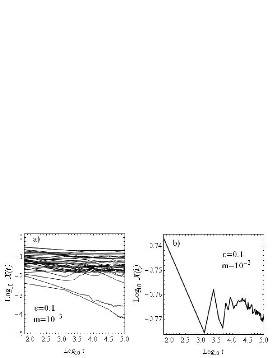
Figure 1: (a)Time evolution of finite Lypunov numbers for the ensemble of orbits in the case $m=10^{-3}$, $\varepsilon=0.1$. (b) The detailed form of the curve $\chi(t)$ for one chaotic orbit (initial conditions $x=0.064$, $y=-0.0625$, $z=-0.123$, $v_{x}=0.064$, $v_{y}=0.028$, $v_{z}=-0.06$. After the time $t=10^{4}$ the variations of $\chi(t)$ are less than 2%.

Almost all orbits in this ensemble are chaotic, as their finite-time Lyapunov exponents are stabilized to non zero values. Only a small subset of orbits exhibit a value of $\chi(t)$ that keeps falling even at the time $t=10^{5}$, following the law $\chi(t)\sim 1/t$. This subset defines regular orbits. The detailed time behaviour of $\log\chi(t)$ for a typical chaotic orbit is shown in Fig.1b. A general remark is that for the entire set of parameter values used in our experiments, the large majority of orbits in our ensembles turn to be chaotic. The minimum percentage of chaotic orbits ($67\%$) is observed in the experiment with the minimum values of $m$ and $\varepsilon$, i.e. $m=10^{-5}$ and $\varepsilon=0.01$. The classification of orbits as ordered or chaotic is based on a ‘Fast Lyapunov Indicator’ criterion (Froeschlé et al. (1997)), namely on whether the length $\xi(t)$ of the deviation vector is smaller, or larger, respectively, than a threshold value set equal to $\xi_{th}(t)=100t$.

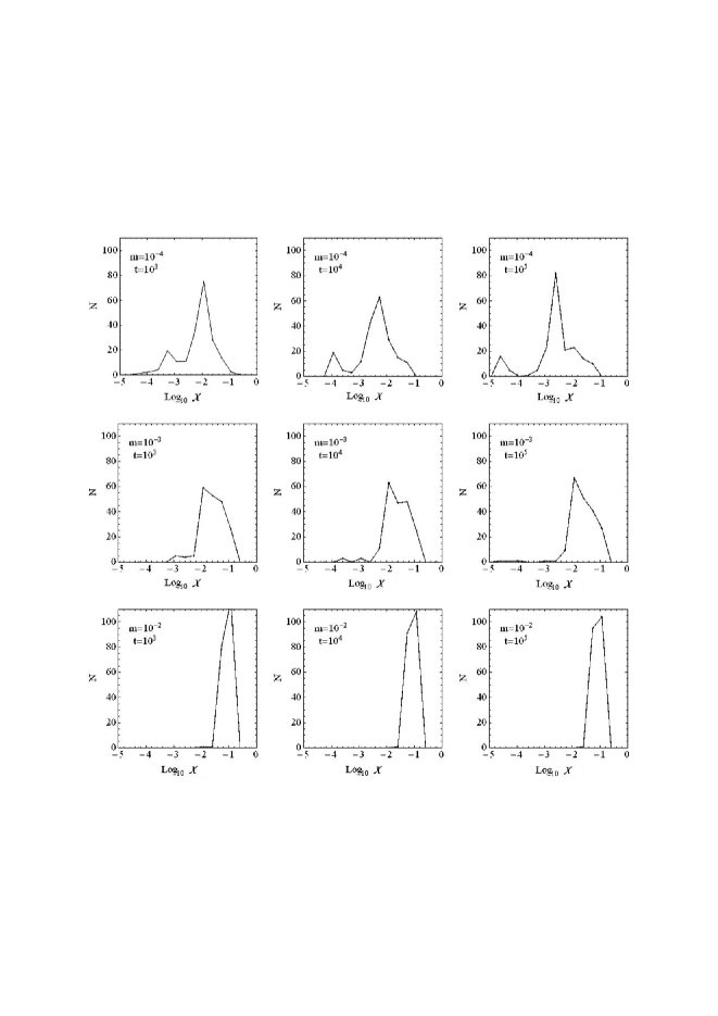
Figure 2: The distributions $P(\log\chi(t))$ for the particles in our ensembles. Every line of histograms corresponds to a different central mass parameter ($m=10^{-4}$, $m=10^{-3}$, $m=10^{-2}$) whereas every column to a different time snapshot ($t=10^{5}$, $t=10^{4}$, $t=10^{3}$). The histograms are shown for $\varepsilon$=0.1.

Figure 2 shows the distribution of the quantity $\log\chi(t)$ for three different time snapshots ($t=10^{3}$, $t=10^{4}$, $t=10^{5}$) for the ensembles of orbits in the experiments with central mass values $m=10^{-4}$, $m=10^{-3}$ and $m=10^{-2}$. In all cases we can see that the distribution $\log{\chi(t)}$ exhibits a main peak corresponding to the chaotic orbits, which is displaced to higher values of $\log{\chi(t)}$ as the central mass $m$ increases. On the other hand, for the mass values $m=10^{-4}$ and $m=10^{-3}$ there appears a secondary peak in the distribution of $\log\chi(t)$, that corresponds to the small subset of regular orbits. The secondary peak is displaced to the left, as the quantity $\log\chi(t)$ for regular orbits decreases in time as $-\log t$. For the largest central mass values ($m=10^{-2}$), however, we observe no secondary peak, i.e., all the orbits turn to be chaotic.

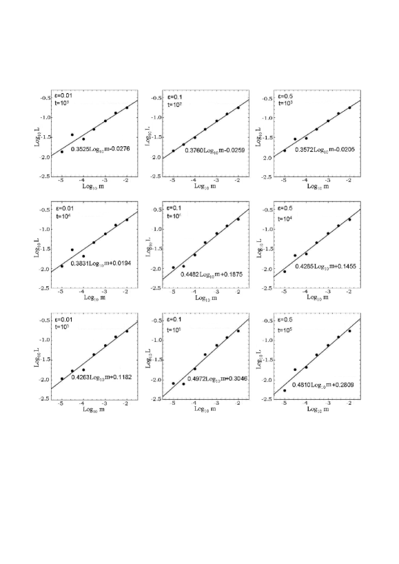
Figure 3: The $L=\overline{\chi(t)}$ versus $m$ relation in logarithmic scale for all our experiments, with parameters as indicated in the panels.

Figure 3 shows the main result. From the histograms of Fig.2, the mean value $L=\overline{\chi(t)}$ is extracted and plotted against $m$ at the snapshots $t=10^{3}$, $t=10^{4}$ and $t=10^{5}$ for all the numerical experiments. The straight lines in the same plots (in logarithmic scale) represent power-law fittings of the relation between $L$ and $m$. The best-fit exponents in different plots range in values between $p\simeq 0.35$ and $p\simeq 0.5$. We also note a tendency towards smaller values for smaller $t$. However, the bigger values are more representative of the true exponent, since they appear at times closer to the limit when $\chi(t)$ tends to its limiting value for chaotic orbits, i.e. the Lyapunov characteristic number (LCN). If $l=\lim_{t\rightarrow\infty}\chi(t)$ denotes the LCN limit, it is well known (see e.g. Kalapotharakos & Voglis (2005)) that the generic behavior of $\chi(t)$ is to fall like $t^{-1}$ up to a time $t_{l}\approx l^{-1}$. The time $t_{l}$ is called ‘Lyapunov time’, and represents a saturation time beyond which the curve $\chi(t)$ starts stabilizing towards the limiting value $l$. The temporal change of $\chi(t)$ for times $t<t_{l}$ is reflected in the histograms of Fig.2. We can observe that, along a fixed panel row (i.e. fixed $m$, integration time increasing from left to right), the right wing of the histogram is shifted in general to the left as $t$ increases. The shift is more conspicuous in the uppermost panel row (small $m$), in which the orbits have, in general, smaller values of the LCN, and hence, larger values of their saturation times $t_{l}$. On the other hand, in the lowermost panel row ($m=10^{-2}$, i.e., large), the saturation time is small ($t_{l}<10^{3}$ for nearly all orbits). Hence, the histogram $N(\chi)$ remains practically invariant beyond the time $t=10^{3}$, as shown in the three panels of the same row.

The difference in the saturation times between small and large $m$ has, as a consequence, that in each column of Fig.3 (same parameters but increasing $t$), the value of $L$ for all $m$ presents some shift downwards as $t$ increases. The shift is important for small values of $m$, while it is nearly negligible for large values of $m$ (for which the orbits reach their saturation times $t_{l}$ already before $t=10^{3}$). Hence, the effective logarithmic slope $p$ increases as $t$ increases. Nevertheless, the tendency of $p$ to increase with time is only temporary, since $p$ is stabilized after all the orbits have reached their saturation times. This happens around $t=10^{5}$.

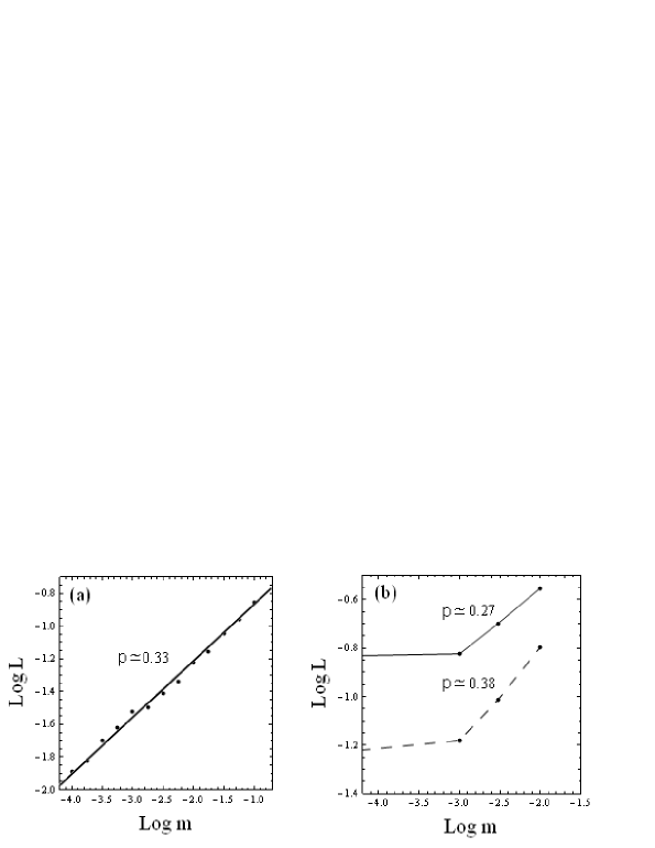
Figure 4: The $L$ versus $m$ relation as derived from the data of (a) Kandrup and Sideris (2002) (lowest order approximation of a triaxial Dehnen potential), and (b) Merritt and Valluri (1996) (potential corresponding to a galaxy with cusp). In (a), the compiled data confirm a power law relation $L\sim m^{p}$ over the whole range of values of $m$ considered. The solid line corresponds to a best fit yielding an exponent $p\simeq 0.33$. In the right panel (b) the solid and dashed lines show the dependence on $m$ of the logarithms of the mean first and second Lyapunov exponents respectively. Both lines extend to a non-zero value of $\log L$ for $m\rightarrow 0$. This represents the values corresponding to what is called ‘residual chaos’ in section 4 below, i.e., chaos induced by the central cusp itself. The best-fit exponents were computed in this case only by the three rightmost data points.

Another remark is that the dependence of the exponent $p$ on the anharmonicity parameter $\varepsilon$ appears to be weak. This fact confirms that the main source of the chaotic behavior of the orbits is the scattering by the central mass, while nonlinear effects due to the quartic terms in the potential are of small importance. This agrees with findings in (Kandrup & Sideris (2002)). It should be noted, in this respect, that a power-law relation $L\sim m^{p}$ can be extracted by an a posteriori analysis of data in independent published works (Kandrup & Sideris (2002), Merritt & Valluri (1996)). In particular, Kandrup & Sideris (2002) computed finite-time Lyapunov Characteristic exponents in a potential representing the lowest expansion terms of a Dehnen potential with a superposed softened Keplerian term corresponding to the central mass. From their work (their figure 12), the relation between $L$ and $m$ can be compiled in a log-log scale. As shown in Fig.4a, one obtains a power law fitting with $p\simeq 0.33$. Similarly, Merritt & Valluri (1996) computed the first and second (finite-time) Lyapunov characteristic numbers of chaotic orbits in potentials corresponding to a galaxy with cuspy density profile and a central core radius. Their results can be compared to ours in the limit where the core radius (their parameter $m_{0}$) is larger than the sphere of influence of the central mass. This is the case $m_{0}=10^{-1}$ in Table 1 of Merritt & Valluri (1996), compiled in log-log scale in Fig.4b. Apart from the value $m=0$ (corresponding to the horizontal line going to $-\infty$), the three available data points appear also to be aligned in straight lines indicating power laws both for the first and the second Lyapunov exponent. The best-fit exponents are $p\simeq 0.27$ and $p\simeq 0.38$ respectively, while these values are only indicative due to the scarcity of data and the unknown influence of the central cusp of the potential to the result. We note, finally, that the breaking of the power law and the appearance of a non-zero value of $L$ as $m\rightarrow 0$ in Fig.4b is due to a phenomenon called below ‘residual chaos’, i.e. chaos due to the cusp itself. This phenomenon is analyzed in section 4.

As an overall conclusion, a power-law $L\sim m^{p}$ appears quite commonly in numerical computations of the Lyapunov exponents of the stellar orbits chaotically scattered by a central mass in various galactic models. We now proceed in a theoretical modelling allowing to interpret the origin of this power law.

3 Theoretical modelling

3.1 Transit and out-of-transit dynamics

As mentioned in the introduction, a modelling of the process of chaotic scattering of the orbits by the central mass becomes feasible by considering two distinct regimes of the motion, i.e. i) transits through the sphere of influence and ii) out-of-transit oscillations. We begin by showing that within the out-of-transit regime the orbits obey three quasi-integrals of motion. Such integrals can be written as formal series, using, for example, the ‘third integral’ approach (Contopoulos (1960)). A formal series has the form $\Phi=\Phi_{2}+\Phi_{3}...$, where $\Phi_{r}$ are polynomial terms of degree $r$ in the canonical variables $(x,y,z,p_{x},p_{y},p_{z})$. The term $\Phi_{2}$ is set equal to the harmonic energy in one of the three possible degrees of freedom, i.e. $(p_{x}^{2}+\omega_{x}^{2}x^{2})/2$, $(p_{y}^{2}+\omega_{y}^{2}y^{2})/2$, or $(p_{z}^{2}+\omega_{z}^{2}z^{2})/2$. Terms of higher degree are computed recursively, by solving, order by order, the equation

$${d\Phi\over dt}=[\Phi,H_{2}+H_{4}]=0$$ (10)

where $[\cdot,\cdot]$ denotes the Poisson bracket operator, and $H_{2}$, $H_{4}$ are the quadratic and quartic terms of the Hamiltonian (3). This means that the formal integrals are possible to define for the Hamiltonian neglecting the influence of the central mass. Then, we test numerically how well they are preserved in the full model, in the out-of-transit regime.

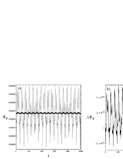
Figure 5: (a) Variations of the value of the formal integral $\Phi_{x}$ truncated at order 4 (thin line) or 10 (thick line) for an example of box orbit with initial conditions $x=0.34$, $y=0.23$, $z=0.21$, $v_{x}=v_{y}=v_{z}=0$. (b) The variations of the order 10 truncated series in greater detail (notice the change of scale in the vertical axis).

Equation (10) yields, at degree $r$, the homological equation

$$[{H_{2},\Phi_{r}}]=[{\Phi_{r-2},H_{4}}]~{}~{}.$$ (11)

We used a computer-algebraic program to solve, step by step, the homological equation, for all three formal integrals defined as the above way, up to the 10th degree in the variables $(x,y,z,p_{x},p_{y},p_{z})$. As an example, for the formal integral $\Phi_{x}=(p_{x}^{2}+\omega_{x}^{2}x^{2})/2+...$ up to 4th degree we have

$${\Phi_{x}} = {0.5x^{2}+0.5p_{x}^{2}}-\varepsilon\bigg{(}0.0025p_{x}^{2}p_{y}^{2}-0.007p_{x}p_{y}^{3}-0.0034p_{x}^{2}p_{y}p_{z}$$ (12)

$$- 0.01p_{x}p_{y}^{2}p_{z}-0.00125p_{x}^{2}p_{z}^{2}+0.0025p_{y}^{2}x^{2}+0.0034p_{y}p_{z}x^{2}$$

$$+ 0.00125p_{z}^{2}x^{2}-0.01p_{x}p_{y}xy-0.007p_{y}^{2}xy-0.0052p_{x}p_{z}xy$$

$$- 0.02p_{y}p_{z}xy-0.0176p_{x}p_{y}y^{2}+0.01p_{x}p_{z}y^{2}-0.0152xy^{3}$$

$$- 0.0086p_{x}p_{y}xz+0.01p_{y}^{2}xz-0.005p_{x}p_{z}xz-0.0017p_{x}^{2}yz$$

$$- 0.04p_{x}p_{y}yz+0.0017x^{2}yz-0.03xy^{2}z-0.00125p_{x}^{2}z^{2}$$

$$- 0.00125x^{2}z^{2}\bigg{)}+O(\varepsilon^{2})~{}~{}.$$

Similar expressions are found for the formal integrals $\Phi_{y}$, $\Phi_{z}$. The degree of approximation of these expressions can be tested by probing how well the integral values are preserved along individual orbits integrated first in the Hamiltonian $H=H_{2}+H_{4}$ (i.e. without the central mass). For orbits in the energy range considered, we find that, up to $r=10$, all three integrals are preserved to within a time variation of about $10^{-(4+r/2-2)}$ at the truncation order $r$. Figure 5 shows an example of this behavior. Panel (a) shows a comparison of the variations of the quantity $\Phi_{x}$, computed as above, at the truncation orders $r=4$ and $r=10$, for an example of box orbit with initial conditions as indicated in the panel. The maximum variation is about $\pm 2\times 10^{-4}$ at the truncation order $r=4$, but it reduces to about $\pm 3\times 10^{-6}$ at the truncation order $r=10$ (magnified in panel (b)). In fact, the estimates of Nekhoroshev theory (see, e.g., Efthymiopoulos et al. (2004)) yield that the variations continue to decrease up to an optimal truncation order $r_{opt}\sim 1/(\varepsilon E)$, in which they become exponentially small, i.e., of order $O(\exp(-1/(\varepsilon E))$. However, even low order truncations are sufficient for estimating the values of the integrals $\Phi_{x}$, $\Phi_{y}$ and $\Phi_{z}$ in practice.

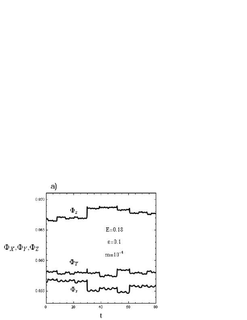
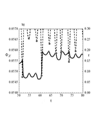
Figure 6: (a) Time evolution of the quantities $\Phi_{x},\Phi_{y},\Phi_{z}$ for one orbit with energy $E=0.18$ in the experiment with $m=10^{-4}$, $\varepsilon=0.1$ (initial conditions as in Fig.5). (b) The time evolution of $\Phi_{x}$ in detail (solid curve, corresponding to the scale of the left vertical axis), along with the time evolution of the orbit’s distance from the center (dashed curve, corresponding to the scale of the right vertical axis). Gray points on the latter curve correspond to local minima, while gray points on the $\Phi_{x}$ curve correspond to local extrema. Note that a local maximum of the curve $\Phi_{x}(t)$ coincides always with a local minimum of the curve $r(t)$.

Restoring, now, the term $-m/(r^{2}+d^{2})^{1/2}$ in the potential, we compute the variation of all three quantities $\Phi_{x},\Phi_{y},\Phi_{z}$ during both transits and the out-of-transit regime. Figure 6a shows the example of an orbit with initial conditions as in Fig.5 (energy $E=0.18$) in the case $m=10^{-4}$, $\varepsilon=0.1$. All three integrals are seen to exhibit abrupt jumps that coincide in time (e.g. at the times $t=30$, $t=52$ or $t=61$ in Fig.6a). A closer focus to the jump at $t=52$ is shown in (Fig.6b), superposing the variations of $\Phi_{x}$ in time with the variations of the distance of the orbit from the center. Clearly, the most important jumps take place during transits through the sphere of influence of the central mass (which is about $2\times 10^{-4/3}\simeq 0.1$ in this case, see below, end of subsection 3.1). A similar behavior is found for the quasi-integrals $\Phi_{y}$, $\Phi_{z}$. On the other hand, the values of all three integrals are preserved to within two significant figures in the out-of-transit regime (without the central mass, the precision increases to about four significant figures at the truncation order $r=4$, see above).

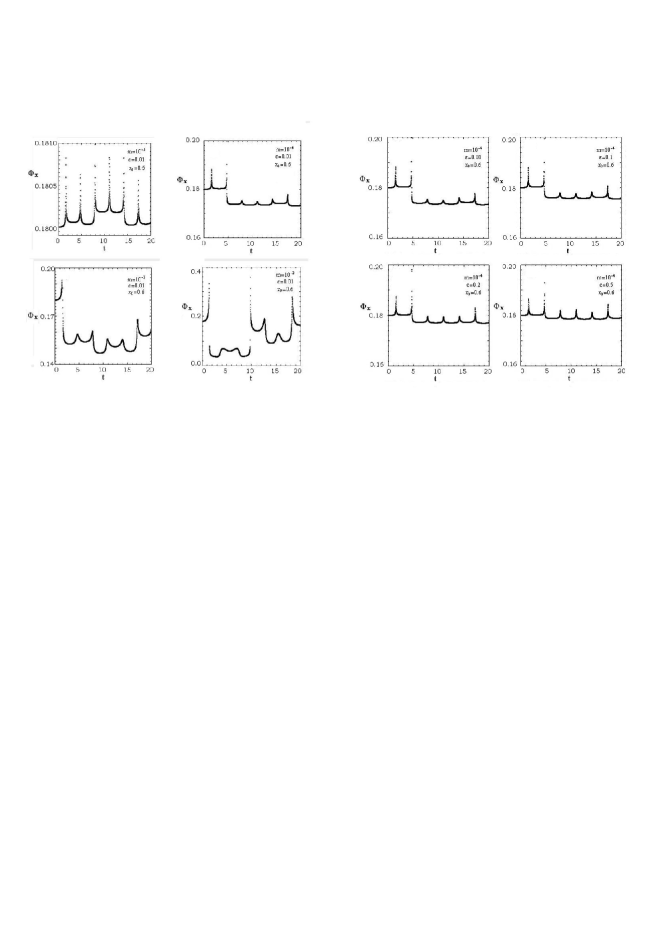
Figure 7: Variations of $\Phi_{x}(t)$ for an orbit with energy $E=0.18$ and four different values of $m$ (left), or $\epsilon$ (right). The values of $(\mu,\varepsilon)$ are indicated in the figure. Note the change of scale in the ordinate of the four left panels, indicating that the variations of the quasi-integral depend strongly on the value of the mass parameter (while they are nearly insensitive to the non-linearity parameter $\varepsilon$ as long as the latter is not very close to unity).

Figure 7, now, compares the variations of $\Phi_{x}(t)$ for an orbit with the same initial conditions but different values of $m$ and $\varepsilon$. The overall size of the variations appears rather insensitive on $\varepsilon$, while the size of all jumps (i.e. the difference between the value of $\Phi_{x}$ at the local maximum and minimum along a jump) clearly increases as $m$ increases. One can observe also that the ‘landing’ value of $\Phi_{x}(t)$ at the end of one jump appears to be more and more unpredictable as $m$ increases. Essentially, this uncertainty in the value of $\Phi_{x}(t)$ after each jump is a measure of the chaoticity of the orbit.

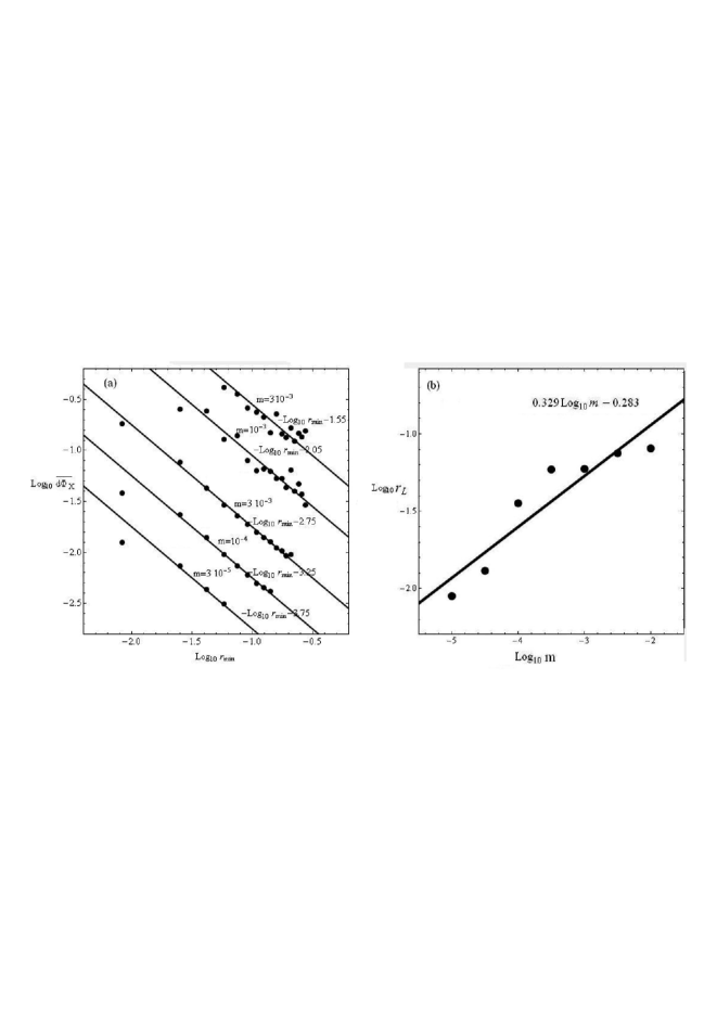
Figure 8: (a) The points represent the logarithm of the mean absolute value of the $\Phi_{x}$ integral’s jumps $\log\overline{d\Phi_{x}}$ for different values of the central mass parameter, versus the logarithm of the mean minimum distance $r_{min}$ from the central mass over all transits for chaotic orbits with initial conditions as in Fig.6. The fitting straight lines have equation as indicated in the figure. (b) The mean radius $r_{L}$ within which the angular momentum is approximately conserved (see text) versus $m$.

Quantifying the behavior of the jumps after many transits allows to see that the scattering of the orbits can be modelled essentially by Keplerian hyperbolic dynamics. Figure 8a shows the mean value of the jumps $d\Phi_{x}$ (measured as the difference between the local maximum and minimum values of $\Phi_{x}$ at each jump) plotted against the mean value of the radii $r_{min}$, where $r_{min}$ (computed from the data of Fig.6b) means the radial distance from the central mass at the point of closest approach during one jump. Both means are taken over the ensemble of all jumps during an integration of an orbit up to a time $t=10^{5}$. The computation is repeated for different central mass values $m$, keeping the orbit’s initial conditions fixed (same as in Fig.6). During this time, the orbit exhibits some thousands of transits, thus the evaluation of mean values for both $d\Phi$ and $r_{min}$ has small statistical error. Figure 8a shows the mean value of $d\Phi_{x}$ as a function of the mean value of $r_{min}$, superposing the plots in log-log scale for the masses $m=3\times 10^{-5}$, $10^{-4}$, $3\times 10^{-4}$, $10^{-3}$, and $3\times 10^{-3}$. The straight fitting lines have inclination -1, whereas we note that the vertical distance between two successive lines is about equal to $\log_{10}3\approx 0.5$. Thus, the mean jump $\overline{d\Phi_{x}}$ is consistent with a (absolute) Keplerian potential law:

$$\overline{d\Phi_{x}}\approx{m\over\overline{r_{min}}}~{}~{}.$$ (13)

The above result concerns the variations of the quasi-integrals valid in the out-of-transit regime. On the other hand, inside the sphere of influence the force field is approximately central, thus another approximate integral, of the angular momentum $\mathbf{L}$, is valid. During transits, we follow the time variations of $\mathbf{L}$ and determine, at each transit separately, the maximum radius $r_{L}$ up to which the variations $\Delta\mathbf{L}$ are smaller in size than a fixed percentage of $\mathbf{L}$ (taken as $10\%$ difference measured from the value of $\mathbf{L}$ at the point of closest approach to the central mass). Figure 8b shows the so-obtained mean value of $r_{L}$ as function of the central mass parameter $m$ in log-log scale for the same orbits as in Fig.8a. Albeit with considerable scatter, the data allow to determine a best-fit power law $r_{L}\approx 2.2m^{0.329}$. This is close to the power law for the sphere of influence (Eq.(5), thus allowing to identify $r_{L}$ as a measure of $r_{m}$ yielding the estimate $r_{c}\approx 2$. We note that the threshold of 10% variation of the angular momentum is rather arbitrary. However, it allows to obtain a meaningful result for box orbits which, far from the BH sphere of influence, undergo angular momentum variations of order 100% (with more stringent thresholds we identify significantly fewer transitions through the BH sphere of influence).

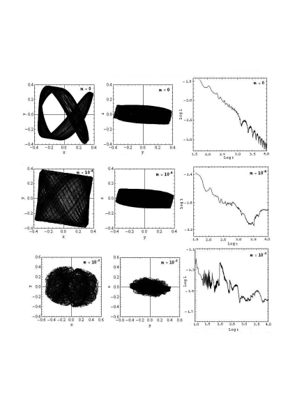
Figure 9: Upper row: projection of a thin tube orbit around a ‘boxlet’ 3:2 periodic orbit in the planes $(x,y)$ (left panel), and $(y,z)$ (middle panel), along with the evolution of its finite-time Lyapunov exponent $\chi(t)$ (right panel). The central mass parameter is set equal to $m=0$, and the nonlinearity parameter $\varepsilon=0.9$. The orbit’s initial conditions are: $x=0.1894$, $y=-0.04796$, $z=0.0014$, $v_{x}=-0.3578$, $v_{y}=-0.4682$, $v_{z}=-0.097$. The orbital energy is $E=0.193$. Middle and lower rows: same as in the upper row, but with a central mass $m=10^{-4}$ and $m=10^{-3}$ respectively.

In conclusion, their scatter notwithstanding, the previous plots suggest a qualitative picture in which the dynamics of chaotically scattered centrophylic orbits can be modelled as a sequence of i) transits through the sphere of influence, in which the orbits follow approximately a Keplerian hyperbolic dynamics, followed by ii) box-like wanderings within the rest of the available space in the interior of the equipotential ellipsoid corresponding to a fixed value of the orbital energy. This picture is quite generic when the three frequencies $\omega_{1}$, $\omega_{2}$, $\omega_{3}$ are far from low-order commensurabilities. The generation of such commensurabilities necessitates a separate treatment, since, then, the orbital sample contains also many resonant boxlets (Miralda-Escudé & Schwarzschild (1989)). In our model, boxlets corresponding to low-order commensurabilities are generated by the quartic potential terms in Eq.(4) for large (${\cal O}(1)$) values of $\varepsilon$. An example is given in Fig.9, for $\epsilon=0.9$. When $m=0$ (top row) the orbit with initial conditions as indicated in the figure’s caption is a three-dimensional thin-tube orbit around a resonant $3:2$ orbit which exists in the plane $(x,y)$. The periodic orbit is stable, and, hence, centrophobic (Merritt & Valluri (1999)). In Fig.9, top row, the tube orbit around the boxlet also avoids the center. Hence, it is a regular orbit, as confirmed by computing its Lyapunov characteristic exponent (right panel), which goes to zero. Now, the orbit’s closest approach to the center is at a distance $r\sim 2\times 10^{-2}$. Thus, by adding a central mass with parameter $m=10^{-4}$ (middle row), the orbit now crosses the central mass sphere of influence (of radius $\sim 10^{-4/3}$). As a result, we observe that the orbit is significantly deformed, and looses its resonant character, while the Lyapunov exponent stabilizes to a positive value $\sim 10^{-2}$, i.e., the orbit becomes weakly chaotic. For still larger $m$ ($m=10^{-3}$), the orbit exhibits the usual behavior of a chaotic centrophylic orbit, with a Lyapunov exponent $\sim 2.5\times 10^{-2}$.

We now model the chaotic scattering process of centrophylic orbits in order to derive theoretical estimates for the orbits’ Lyapunov exponents.

3.2 Theoretical Estimates on Lyapunov Exponents

Consider an orbit integrated along with the variational vector $\mathbf{\xi}(t)$ of a nearby orbit up to the time $t$. Let $\xi_{i}$ be the modulus of the deviation vector of the orbit at the time $t_{i}=i\Delta t$, where $\Delta t=t/n$ is the timestep corresponding to a splitting of the integration in $n$ steps. The stretching number Voglis & Contopoulos (1994) at the i-th step is defined as

$$a_{i}={1\over\Delta t}\ln{\xi_{i}\over\xi_{i-1}}~{}~{}.$$ (14)

The finite time Lyapunov characteristic number is equal to the mean stretching number along the orbit, since

$$\chi(t)={1\over t}\ln{\xi(t)\over\xi_{0}}={1\over{n\Delta t}}\sum_{i=1}^{n}\ln{\xi_{i}\over{\xi_{i-1}}}={1\over n}\sum_{i=1}^{n}a_{i}~{}~{}.$$ (15)

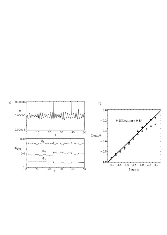
Figure 10: (a) Comparison of the time evolution of the stretching number $a(t)$ (Eq.(14)) with the variations of the quasi-integrals $\Phi_{x}$, $\Phi_{y}$, $\Phi_{z}$. (b) The mean stretching number $\overline{a}$ after thousands of transits versus $m$ for the orbit with same initial conditions as in Fig.6. A power-law fit yields $\overline{a}\propto m^{0.28}$. The theoretical estimate $\overline{a}\propto m^{1/3}$ is found in the appendix.

Figure 10a shows the time evolution of the stretching number $a(t)$ as a function of time, along with the variations of the integral $\Phi_{x}(t)$ for the orbit with initial conditions as in Fig.7, for $m=10^{-3}$, $\varepsilon=0.1$. Far from transits, the function $a(t)$ shows an oscillatory behavior around zero. This behavior is characteristic of a nearly-harmonic oscillation, while the quartic potential term implies an overall linear growth of the deviation vector in the out-of-transit regime, which is of order $O(\varepsilon)t$. On the other hand, in Fig.10a the curve $a(t)$ clearly exhibits positive peaks at all transits.

Consider the set ${\cal S}=\{i_{1},i_{2},...,i_{n_{T}}\}$ such that the orbit is in transit at the time $t_{i}$ with $i\in S$, $n_{T}$ denoting the total number of timesteps during which the orbit is in the transit phase. Let $\overline{{\cal S}}$ be the complement of ${\cal S}$ with respect to the set $\{1,2,...,n\}$. One has the estimate:

$${1\over{n\Delta t}}\sum_{i_{j}\in\overline{{\cal S}},j=1}^{n-n_{T}}\ln{\xi_{i_{j}}\over{\xi_{i_{j}-1}}}\approx O\left({\ln(\varepsilon n\Delta t)\over n\Delta t}\right)$$

implying that the contribution of the ‘out-of-transit’ stretching numbers to the final value of $\chi(t)$ goes to zero as $\sim\ln t/t$. Thus, one has the approximation

$$\chi(t)\approx{1\over{n\Delta t}}\sum_{i_{j}\in{\cal S},j=1}^{n_{T}}a_{i_{j}}~{}~{}.$$

Setting $\overline{a}=(1/n_{T})\sum_{i_{j}\in{\cal S},j=1}^{n_{T}}a_{i_{j}}$ we get $\chi(t)\approx(n_{T}/n\Delta t)\overline{a}$. The quantity

$$N_{vis}={n_{T}\over n\Delta t}$$

hereafter called ‘rate or visits’, represents the number of transits per unit period of an orbit whithin the sphere of influence. We then have

$$\chi(t)\approx N_{vis}\overline{a}~{}~{}.$$ (16)

Estimates on the mean value of $\chi(t)$ for all transiting orbits at fixed central mass parameter $m$ will then follow by estimating separately the quantities $\overline{a}$ and $N_{vis}$.

Assuming, as evidenced above, that the transits are governed by nearly-Keplerian hyperbolic dynamics, in the Appendix it is shown that for orbits of given energy $E$, one has the theoretical estimate

$$\overline{a}\propto{m^{1/3}\over E^{1/2}}~{}~{}.$$ (17)

Figure 10b shows the mean $a$ computed numerically for an orbit of fixed energy with the same initial conditions as in Fig.6, integrated under various values of $m$. Numerically we find the exponent 0.28, which is in fair agreement with the theoretical exponent $1/3$ of Eq.(17). The predicted dependence of $\overline{a}$ on the energy, probed numerically below, is also verified.

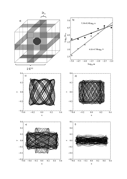
Figure 11: (a) Schematic representation of the configuration space of motion of “3D-orbits” and “planar” orbits. The cube represents a box volume covered by a “3D-orbit”. The central sphere represents the central mass sphere of influence. The three thin parallelepipeds (gray) correspond to one parallelepiped side being equal to $2r_{m}$. Planar orbits are orbits lying inside one of the three parallelepipeds. (b) The number of visits (up to time $t=10^{5}$) versus $m$ for two orbits characterized as ‘3D’ (black points, initial conditions $x=0.227$, $y=0.155$, $z=0.139$, $v_{x}=v_{y}=v_{z}=0$), and ‘planar’ (gray points, initial conditions $x=0.227$, $y=0.155$, $z=0.0$,$v_{x}=v_{y}=v_{z}=0$), for $\varepsilon=0.1$. The straight lines represent power-law fittings yielding the best-fit exponents 0.7 and 0.34 respectively. (c-d) Projection of the ‘3D’ orbit in the planes $(x,y)$ and $(x,z)$. (e-f) Same for the ‘planar’ orbit. Note in (e) the change in morphology induced by a big jump in the values of the quasi-integrals $\Phi_{x}$, $\Phi_{y}$. Such jumps are stochastic in nature, and they may occasionally convert a 3D orbit to planar and vice versa.

We now focus on estimating $N_{vis}$. The frequency whereby an orbit visits the sphere $r_{m}$ depends on the geometry of the orbit in configuration space. We distinguish two cases, explained with the help of Fig.11:

i) 3D-orbit: as long as the three quantities $\Phi_{x}$, $\Phi_{y}$, $\Phi_{z}$ obtain comparable values, an orbit fills nearly uniformly the available configuration space, which has the form of a deformed 3D box.

ii) planar orbit: at least one of the three quantities $\Phi_{x}$, $\Phi_{y}$, $\Phi_{z}$ obtains a value smaller than a given threshold (given by Eq.(18) below). Geometrically, the amplitude of oscillations in at least one of the three axes in the out-of-transit regime should be smaller than the radius $r_{m}$ of the sphere of influence (Fig.11a, schematic). Quantitatively

$$(2\Phi_{k}/\omega_{k}^{2})^{1/2}<r_{m}$$ (18)

where $k$ stands for $x$, $y$, or $z$.

Note that ‘linear’ orbits, i.e., tubes around the stable axial orbits also exist, but their importance is rather limited because they are considerably fewer than the planar or 3D orbits.

The dependence of the rate of visits to the central masses’ sphere of influence on the geometry of orbits can be modelled in the following way: for 3D-orbits, considering all possible straight line segments connecting two different points on the surface of the box delimiting the orbit (see Fig.11a), $N_{vis}$ can be approximated as proportional to the percentage or line segments passing through the sphere of influence. Then, $N_{vis}\propto S_{r_{m}}/S_{tot}$, where $S_{r_{m}}$ and $S_{tot}$ are the surface of the sphere of influence and of the box respectively. The linear dimension of the box is of order $l\sim E^{1/2}$, where $E$ is the energy of the orbit. Thus, $N_{vis}\propto r_{m}^{2}/E$, or (taking into account Eq.(5))

$$N_{vis}\propto{m^{2/3}\over E}~{}~{}.$$ (19)

For planar orbits, one has, instead, the estimate $N^{\prime}_{vis}\propto r_{m}/l$, or

$$N^{\prime}_{vis}\propto{r_{m}\over E^{1/2}}={m^{1/3}\over E^{1/2}}~{}~{}.$$ (20)

These estimates are confirmed numerically. Fig.11b shows a computation of the rate of visits $N_{vis}$, $N_{vis}^{\prime}$ for two orbits with constant energy $E=0.18$, but for different mass parameters $m$. The number of visits within a total integration time $t=10^{5}$ are counted, and criterion (18) is used in order to distinguish either orbit as ‘planar’ or 3D (the corresponding rate of visits is found by dividing the number of visits by $t=10^{5}$). The difference in the shape of the orbits is evident (Figs.11c-f). Returning to Fig.11b, the best-fit exponents of the relations $N_{vis}$ and $N_{vis}^{\prime}$ to $m$ are 0.7 and 0.34 respectively, in fair agreement with Eqs.(19) and (20) for constant $E$.

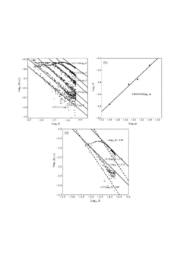
Figure 12: (a) The logarithms of finite-time Lyapunov characteristic numbers $\log\chi$ of all orbits in the choosen ensembles versus the logarithm of the orbital energy $\log E$ for the experiments with mass parameters (from top to bottom) $m=10^{-2}$, $m=3\times 10^{-3}$, $m=10^{-3}$, $m=3\times 10^{-4}$, $m=10^{-4}$ and $m=3\times 10^{-5}$, at the end of the integration ($t=10^{5}$). The straight lines represent asymptotic power-law fittings for the right parts of the plots separately for each mass parameter. (b) The energy $E_{max}$ where $\log\chi$ in (a) exhibits a global maximum versus $m$. The power-law fiting is $E_{max}=2.2{m^{2/3}}$. (c) The plot $\log{\chi}$ versus = $\log E$ in greater detail for the masses $m=3\times 10^{-3}$, and $m=3\times 10^{-4}$. In each case, numerical values are distributed between two lines with inclination -1 and -1.5, as predicted from Eqs.(22) and (21) for the planar and the 3D orbits respectively.

Taking into account eqs.(20),(19) and (17) we find for the Lyapunov number of 3D-orbits of energy $E$ the estimate:

$$\chi\approx{m^{2/3}\over E}\times{m^{1/3}\over E^{1/2}}\approx{m\over E^{3/2}}$$ (21)

whereas, for planar orbits

$$\chi^{\prime}\approx{m^{1/3}\over E^{1/2}}\times{m^{1/3}\over E^{1/2}}\approx{m^{2/3}\over E}~{}~{}.$$ (22)

Figure 12a shows the values of $\log\chi$ against $\log E$ for all the orbits in our considered ensembles for six different values of the mass parameter $m$ as indicated in the caption. The various ensembles are clearly distinguished by the concentration of points in the scatter plot, the uppermost concentration corresponding to the ensemble in the experiment with the highest mass parameter ($m=10^{-2}$). Each ensemble can be roughly described as consisting of a ‘rising’ and a ‘falling’ part of the value of $\log\chi$ vs. $\log E$. The two parts meet at a point of maximum of $\log\chi$. The position of the maximum moves to the right with respect to $\log E$ as $m$ increases. However, the level value of $\log\chi$ at the maximum remains remarkably constant, i.e. nearly independent of $m$.

The straight lines show power law fittings of $\chi$ with $E$ for the falling part. Despite the large scatter of the data points, we find indicative logarithmic slopes lying in the range between -1 and -1.5 for all ensembles considered. This behavior will be explained below. A power-law roughly holds also in the rising part. The point of maximum corresponds to about the point where the associated best-fit power laws intersect. The intersection point defines an energy $E_{c}$. Computing and plotting $E_{c}$ against $m$ yields approximately a power-law $E_{c}\propto m^{0.63}$ (Fig.12b).

These features can be understood by the following considerations: first, one can note that the left part represents regular or sticky chaotic orbits which have the morphology of pyramids (Merritt & Vasiliev (2011)), i.e. they lie nearly entirely within the sphere of influence of the central mass. Such orbits can be described by perturbations to the Keplerian dynamics of the central mass. The limiting energy value $E_{l}$ up to which an orbit lies entirely within the radius $r=r_{m}$ can be estimated by requiring that the sphere $r=r_{m}$ constitutes the surface of zero-velocity. The estimate

$$E_{l}\approx{1\over 2}\Omega^{2}{r_{m}^{2}}-{m\over r_{m}}\approx{1\over 2}\Omega^{2}r_{c}^{2}{m^{2/3}}-{m^{2/3}\over r_{c}}=\left({r_{c}^{2}\Omega^{2}\over 2}-{1\over r_{c}}\right)m^{2/3}$$ (23)

holds, where $\Omega$ is a geometric-mean estimate of the harmonic frequencies, bounded by the highest of the three frequencies $\omega_{x},\omega_{y},\omega_{z}$. The dependence of $E_{l}$ on $m$ in Eq.(23) has the exponent $0.66$, close to the exponent in the numerical fitting of $E_{c}$ versus $m$ (Fig.12b). This suggests that $E_{l}\simeq E_{c}$ (the near equality holds also checking numerical vs. theoretical coefficients). Use of the estimate (23) is made in the next subsection.

On the other hand, most chaotic orbits lie beyond the energy $E_{max}$. In fact, isolating the plots $\log\chi$ vs. $\log E$ (Fig.12c) for two values of the mass parameter $m$ allows to see that the whole ensemble of orbits in the right wing are delimited between two limiting lines with inclinations -1 and -1.5 respectively, i.e. as predicted from the estimates of Eqs. (22) and (21) for the planar and the 3D orbits respectively. The coexistence of ‘planar’ and ‘3D’ orbits explains in this way the scatter in the data points of Fig.12a.

3.3 Final theoretical estimates: the power law $L\propto m^{p}$

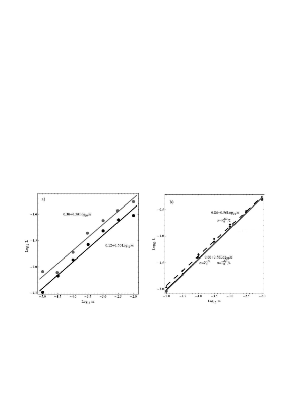
Figure 13: (a)Mean finite Lyapunov characteristic number $L$ vs. the mass parameter $m$ as it follows theoretically from Eq.(28) (black dots), compared to the numerical computation (gray dots) at the integration time $t=10^{5}$, for all the experiments with $\varepsilon=0.1$. The mean inclination is close to 0.5 in the range $10^{-5}<m<10^{-2}$. (b) Theoretical computation of $L$ versus $m$ in a ‘isothermal’ number density model (see text). The triangles and gray fitting line correspond to the choice $\sigma=V_{0}^{1/2}/4$, filled circles and black solid line to $\sigma=V_{0}^{1/2}/2$, squares and dashed line to $\sigma=V_{0}^{1/2}$.

Assuming (as evidenced in Fig.1b) that a time $t=10^{5}$ is sufficient for a saturation of $\chi(t)$ close to the limiting value of chaotic orbits, i.e. close to the Luapunov characteristic number (LCN), the mean LCN of the orbits in an energy range $E_{min}\leq E\leq E_{max}$ can be estimated as

$$L\approx{1\over N_{0}}\int_{E_{min}}^{E_{max}}N(E)\overline{\chi}(t=10^{5},E)dE$$ (24)

where $N_{0}=\int_{E_{min}}^{E_{max}}N(E)dE$, $N(E)$ is the number density of orbits of energy $E$, and $\overline{\chi}(t=10^{5},E)$ is a mean estimate of the value of $\chi$ for orbits of energy $E$ at the final integration time. Considering only transiting orbits, we set $E_{min}=E_{l}\sim m^{2/3}$ (Eq.(23)). Also, from Fig.12a it is clear that the maximum energy $E_{max}=0.2$ considered in our samples is sufficiently high for the orbits’ values of $\chi$ to fall with respect to the maximum by at least one order of magnitude in the worst case ($m=10^{-2}$), and typically by several orders of magnitude.

The mean value $\overline{\chi}(t=10^{5},E)$ can be now estimated by considering the separate mean values of $\chi$ as well as an $E$-dependent varying proportion of planar vs. 3D orbits. The percentage $\lambda$ of the planar orbits is estimated by the ratio of the surface occupied by initial conditions of planar orbits on the box surface corresponding to an energy level $E$ (see Fig.11a) over the total area of the box. Thus

$$\lambda={S_{2d}\over{S_{tot}}}\approx{{48E^{1/2}r_{m}}\over{24E}}\approx{{2m^{1/3}}\over{E^{1/2}}}~{}~{}.$$ (25)

The percentage of 3D orbits is $1-\lambda\approx{1-{2m^{1/3}}/{E^{1/2}}}$. Finally, $\overline{\chi}$ is estimated according to Eqs.(21), (22), i.e.

$$\overline{\chi}_{planar}(E)\approx c_{1}{{m^{2/3}}\over E},~{}~{}~{}\overline{\chi}_{3D}(E)\approx=c_{2}{m\over E^{3/2}}$$ (26)

with $c_{1}$ and $c_{2}$ being constants of order unity. Then, for the mean value of $\chi$ at fixed energy we have the estimate

$$\overline{\chi}(E)\approx\lambda\overline{\chi}_{planar}(E)+(1-\lambda)\overline{\chi}_{3D}(E)~{}~{}.$$ (27)

The main uncertainty in Eq.(24) regards the form of the number density function $N(E)$. In self-consistent models, $N(E)$ is determined by the distribution function of the centrophylic orbits. On the contrary, in ‘ad hoc’ potential models, $N(E)$ cannot be determined self-consistently unless one possesses information on the kinematic distributions allowing to solve the reverse problem $density\rightarrow N(E)$. Assuming no detailed model, we hereby estimate the integral of Eq.(24) using two different estimates of $N(E)$ as follows:

i) we consider the case of a nearly uniform distribution $N(E)=const$. Combining Eqs.(24), (27) and (26) we obtain:

$$L\approx{1\over{0.2-m^{2/3}}}{{[4c_{1}m^{2/3}+10c_{2}m^{4/3}-2.23(4c_{1}+2c_{2})m]}}~{}~{}.$$ (28)

The exact dependence of $L$ on $m$ in the model (28) depends on the relative values of the constants $c_{1}$ and $c_{2}$, as well as on factors entering in all the above estimates. Figure 13a shows $L$ against $m$ in logarithmic scale, by the estimate (28) (black points) setting simply $c_{1}=c_{2}=1$. The plot indicates an approximate power-law $L\sim m^{p}$. This is produced as follows: since $m$ is a small quantity, the leading term in Eq.(28) is the one with lowest exponent, i.e., $m^{2/3}$. Thus, in the absence of additional terms, we would have $p=2/3$. However, for relatively large $m$, the second most important term (linear in $m$) has a negative sign. Thus, it lowers the rightmost part of the curve $L$ vs. $m$ (the presence of $m^{2/3}$ in the denominator only marginally affects the overall power-law behavior). If we approximate the new curve by a single power-law fitting, we then find a lowering of the exponent $p$, i.e.

$$L\propto m^{2/3-q}$$ (29)

with $q$ varying between 0.1 and 0.2. However, one notices that the whole curve in log-log scale deviates downwards from the power-law approximation (29) for the highest mass parameter values, i.e. $q$ has a weak (increasing) dependence on increasing $m$. Comparison with the numerical data (gray dots, for $\varepsilon=0.1$) shows that the model reproduces the slope of the numerical curve, which also exhibits a lowering of the value of $L$ at high mass parameter values with respect to an exact power law. Overall, the theoretical curve has a factor $\approx 2$ difference from the numerical curve, which is consistent with uncertainties in the theoretical coefficients. Notice also that a systematic lowering of the values of $L$ with respect to a power-law fitting is discernible in all the plots of Fig.3. Finally, we have checked that the appearance of an approximate power-law persists, with exponents around $p\approx 0.5$, for different choices of the constants $c_{1}$ and $c_{2}$. This shows that the dependence of the integral (24) on $m$ (which enters in the integral as a parameter) is not sensitive on the details of the distribution of the planar vs. 3D orbits.

ii) Fig.13b shows an evaluation of the integral (24) for an isothermal (or ‘ergodic’, see Binney & Tremaine (2008)) model of $N(E)$, i.e. $N(E)\propto e^{-E/\sigma^{2}}$. The constant $\sigma$ is a measure of the velocity dispersion in the central parts of the galaxy. Assuming a core density $\rho\approx 3/(4\pi)$ (in our units, corresponding to total mass $M=1$ at radius $R=1$), by the Virial theorem $\sigma^{2}$ has to be taken of the order of the absolute value of the central potential well $V_{0}\approx\int_{0}^{1}4\pi G\rho rdr\approx 1.5$. Figure 13b shows the evaluation of the integral (24) for three different choices of $\sigma$, namely $\sigma=V_{0}^{1/2}$, $\sigma=(1/2)V_{0}^{1/2}$ and $\sigma=(1/4)V_{0}^{1/2}$. In all three cases we recover here as well an effective power-law behavior, with not very different exponents, i.e. $p\simeq 0.58$, $p\simeq 0.56$ and $p\simeq 0.56$ respectively.

In conclusion, we find that an approximate power-law relation of the form (29) is robust against details of the form of the function $N(E)$.

4 Effect of central cusp

In the model (4), the existence of many box orbits was a priori guaranteed due to the harmonic core in the center. It is well known, however, that realistic models of the central parts of galaxies include central density cusps $\rho(r)\sim r^{-\gamma}$ (see e.g. the review in Binney & Merrifield (1998), or Merritt (1999)). In such models, the cusp itself transforms most centrophylic orbits to chaotic (Merritt & Valluri (1996), Merritt & Quinlan (1998)). Even without central black hole, one then expects the orbits to exhibit positive Lyapunov exponents. We hereafter call this effect ‘residual chaos’, i.e. chaos existing even when $m=0$. The corresponding mean Lyapunov exponent of the centrophylic orbits is denoted by $L_{0}$.

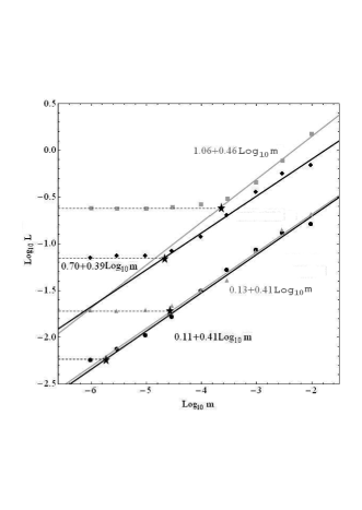
Figure 14: The mean Lyapunov exponent versus the central mass parameter $m$ in four Dehnen triaxial models with central cusps (see text). Black filled circles correspond to the data points for the cusp exponent $\gamma=0.3$, gray triangles to $\gamma=0.7$, black rombuses to $\gamma=1.3$, and gray squares to $\gamma=1.7$. The straight lines (black or gray) are power law fittings obtained by the rightmost seven points for $\gamma=0.3$, five points for $\gamma=0.7$, five points for $\gamma=1.3$, and four points for $\gamma=1.7$. The horizontal dashed lines correspond the the values $\log_{10}L_{0}$, where $L_{0}$ is the ‘residual Lyapunov exponent’ in each case (see text). The points where each horizontal line intersects the fitting line for the same corresponding $\gamma$ are marked as stars.

Adding, now, a central mass ($m\neq 0$) we seek to determine the dependence of $L$ on $m$. The theoretical analysis of the previous section formally breaks down, since one cannot define the formal integrals $\Phi_{x},\Phi_{y},\Phi_{z}$ even for $m=0$. We thus rely on numerical computations. To this end, we consider again the Hamiltonian function (3), changing the potential model to

$$V=V_{D}-{m\over(r^{2}+d^{2})^{1/2}}$$ (30)

where $V_{D}$ represents the ellipsoidal Dehnen model (Dehnen (1993)):

$$V_{D}(x,y,z)=-\pi Gabc\int_{0}^{\infty}{[\psi(\infty)-\psi(w)]d\tau\over\sqrt{(\tau+a^{2})(\tau+b^{2})(\tau+c^{2})}}$$ (31)

where

$$\psi(w)=\int_{0}^{w^{2}}\rho(w^{\prime 2})dw^{\prime 2}$$

with

$$w^{2}={x^{2}\over a^{2}}+{y^{2}\over b^{2}}+{z^{2}\over c^{2}},~{}~{}~{}a\geq b\geq c>0$$

and $\rho(w)$ given by

$$\rho(w)={(3-\gamma)M\over 4\pi abc}w^{-\gamma}(1+w)^{-4+\gamma}~{}~{},~{}~{}~{}~{}0\leq\gamma<3~{}~{}.$$ (32)

The parameters $a$, $b$ and $c$ correspond to the lengths of the major, intermediate and minor axis of the triaxial equipotential surface corresponding to $w=1$. The parameter $M$ determines the system’s total mass. We use a similar algorithm as in Merritt & Fridman (1996) in order to numerically evaluate the integral (31) as well as its spatial derivatives, i.e., the forces.

A ‘weak cusp’ corresponds to $\gamma<1$. In this case, the modulus of any component of the force generated by $V_{D}$ goes to zero at the center, reaches a maximum value at a certain distance from the center, and then falls-off tending to zero at large distances by a Keplerian law. This behavior of the force allows to determine values of the parameters $a$, $b$, $c$, and $M$, for fixed $\gamma$, so as to create a system exhibiting a similar geometry and value of the total mass as the simplified system corresponding to the potential (4) of section 2, the two systems being, hence, differentiated essentially only by the presence of a central cusp as opposed to a harmonic core respectively. The parameter determination is realized by the following algorithm:

i) We set the ratios $a:b=\omega_{y}:\omega_{x}$ and $a:c=\omega_{z}/\omega_{x}$, where $\omega_{x}$, $\omega_{y}$, and $\omega_{z}$ are the parameters of (4).

ii) We fix the value of $a$ so that the quantity $\partial V_{D}/\partial x$ presents maximum at the point $(x=x_{max},y=0,z=0)$, with $x_{max}$ choosen so as to represent the point where the harmonic model in (4) yields a total mass equal to unity. We find $x_{max}\simeq 1.06$.

iii) We fix $M$ so that the force $F_{x}$ under the potential $V_{D}$ be equal to the force $F_{x}$ under the potential (4), with $m=0$, at the point $(x=x_{max},y=0,z=0)$. Note that, since the value of the force depends essentially only on the total mass inside a given radius, this normalization means also that the total mass inside an ellipsoidal surface crossing $x=x_{max}$ is nearly equal in the harmonic and in the $\gamma$–models.

We examine two values of $\gamma$ in the weak cusp case, namely $\gamma=0.3$ and $\gamma=0.7$.

In the case, now, of a ‘strong cusp’ ($\gamma>1$), criterion (ii) can no longer be implemented, since $\partial V_{D}/\partial x\rightarrow\infty$ as $x\rightarrow 0$ (with $y=z=0$), implying that the quantity $\partial V_{D}/\partial x$ does not present any smooth maximum along any of the principal axes. As a simple (but somewhat arbitrary) way to bypass this difficulty, we keep $a$ constant to the value $a=6.67$ found by criterion (ii) in the second ‘weak cusp’ experiment ($\gamma=0.7$). Then, we fix the remaining constants by criteria (i) and (iii). We run also two strong cusp experiments, with $\gamma=1.3$ and $\gamma=1.7$.

In all four experiments, the initial conditions are choosen as in section 2, namely 200 initial points of zero velocity randomly distributed on equipotential surfaces with $V=E$ and $E$ choosen uniformly in the range $0\leq V\leq E_{max}$, with $E_{max}$ choosen as $E_{max}=V_{D}(x_{max})$, so as to ensure that the resulting centrophylic orbits exhibit oscillations of amplitude at most equal to $x_{max}$. However, here we integrate the orbits only up to $t=1000$, since the complexity of force evaluation in the model $V_{D}$ renders the computational cost of longer integration prohibitive. Yet, as shown below, our smallest found Lyapunov exponents are about $L\approx 10^{-2.5}$, implying that a time $t=10^{3}$ is marginally greater than the saturation time $t\sim 1/L$ even for the orbits with smallest Lyapunov exponents.

Figure 14 (analogous to Fig.3, top row) shows the mean Lyapunov number $L=\overline{\chi}(t=10^{3})$ for our ensembles of orbits in the four above experiments, as a function of the central mass parameter $m$. We note immediately that power-law fittings are possible in only a range of values of $m$, i.e. above a critical threshold value $m>m_{c}(\gamma)$. In Fig.14, an estimate of the threshold value is found by the abcissa of the points displayed by stars. They are computed as follows: the four inclined lines represent power-law fittings for the rightmost part of the numerical curve of $L$ vs. $m$ in each experiment. The horizontal lines illustrate the level values of the quantity $L_{0}=L(m=0)$. We call $L_{0}$ the ‘residual Lyapunov exponent’. It represents the mean Lyapunov exponent of the centrophylic orbits when $m=0$, i.e., under the influence of the central cusp only. The point at which a horizontal line of fixed $L_{0}$ intersects the corresponding inclined fitting line of $L$ vs. $m$ in the same experiment (same $\gamma$) marks the position of a star-point, and the associated abscissa, i.e. a critical mass value $m_{c}$. From Fig.14 it is straightforward to see that both $L_{0}$ and $m_{c}$ increase in general with the strength of the cusp (i.e. the value of $\gamma$). On the other hand, it is clear from the numerical data points that an approximate power-law correlation between $L$ and $m$ persists, in all four experiments, for central mass parameters larger than $m=m_{c}$. A physical understanding of this phenomenon is the following: the chaotic scattering caused by the cusp itself acts dynamically as a central mass concentration, whose distribution is not point-like but follows the cusp density law. As long as the BH mass is small, the effect of the cusp is dominant over the efect of the BH. Thus, the mean Lyapunov exponent of the centrophilic orbits remains nearly equal to the residual Lyapunov exponent $L_{0}$. But beyond the BH mass scale $m=m_{c}$, the black hole dominates over the central cusp. Then, we recover a correlation of $L$ with $m$. This goes asymptotically to an effective power-law. Furthermore, the exponents found by fitting in the range $m>m_{c}$ are all about $p\simeq 0.4$, i.e., not very different from those of the corresponding data in Fig.3, the essential difference in the two plots being with respect to whether or not we observe a a critical mass scale in which the power-law breaks.

We note finally, that despite the sparsity of their datapoints, the results of Merritt & Valluri (1996), reproduced here as Fig.4b, show essentially the same structure as the results of Fig.14. Thus, the residual chaos phenomenon explains the plateau of the curve $L$ vs. $m$ in the data of Merritt & Valluri (1996) as well.

5 The $L\propto m^{p}$ law in disc-barred galaxies

N-body simulations of barred galaxies (e.g. Friedli & Benz (1993), Friedli (1994), Norman et al. (1996)) have demonstrated that the growth of a central mass concentration induces secular evolution in such systems as well. In fact, although dynamically not favored, black hole growth to a mass level as high as $10^{8}M_{\odot}$–$10^{9}M_{\odot}$, corresponding to a few percent of the mass of a typical galactic bar, could induce even a total destruction of the bar, with its conversion into a nearly axisymmetric bulge-like component. Test particle integrations in barred potentials (Pfenniger (1984), Pfenniger & de Zeeuw (1989), Hasan et al. (1993)), Norman et al. (1996), Shen & Sellwood (2004), indicate that a primary mechanism responsible for the secular evolution of bars, and even bar dissolution, is chaos induced by the central mass.

Hereafter we study the dependence of Lyapunov exponents on the central mass paramerer in rotating disc-barred galaxies. Two points should be immediately emphasized: i) our modeling in previous sections was based on the existence of box-like centrophilic chaotic orbits. Such orbits cannot exist in rotating disc-barred galaxies. However, as shown in the sequel, centrophilic orbits appear around the main families of planar periodic orbits (e.g. the $x_{1}$ family). Note that the presence of some type of centrophilic orbits is an indispensible feature of bars with a rising density profile in the center. As discussed below, albeit different in morphology, the centrophilic orbits in barred galaxies are found numerically to exhibit a similar chaotic behavior as the boxy centrophilic orbits in elliptical galaxies. ii) Besides the central mass, chaos is generated by the interaction of resonances in the corotation domain (Contopoulos (1981), Pfenniger (1984), Sparke & Sellwood (1987), Pfenniger & Friedli (1991), Kaufmann & Contopoulos (1996), Patsis et al. (1997), Fux (2001), Pichardo et al. (2004), Kaufmann & Patsis (2005)). Nevertheless, this type of chaos is a quite distinct phenomenon. In fact, most chaotic orbits in the corotation domain belong to the so-called ‘hot population’ (Sparke & Sellwood (1987)), hence they are not centrophilic.

5.1 Potential model

As a case study, we employ the barred-galaxy potential introduced by Kaufmann & Contopoulos (1996) in a rough self-consistent modelling of the galaxy NGC3992. Adding a component for the central mass, the total potential is analyzed as:

$$V_{tot}=V_{bh}+V_{h}+V_{d}+V_{b}$$ (33)

where $V_{bh}$ is the potential generated from the central mass (black hole), while $V_{h}$, $V_{d}$, $V_{b}$ are dark halo, disc, and bar potential components respectively. The potential of the central mass is, as before,

$$V_{bh}=-{m_{bh}\over{\sqrt{r^{2}+d^{2}}}}~{}~{}.$$ (34)

The remaining terms are as in Kaufmann & Contopoulos (1996). The dark halo term is

$$V_{h}(r)={{-M_{h}}\over{\sqrt{r^{2}+b_{h}^{2}}}}~{}~{}.$$ (35)

The disc term corresponds to an exponential disc:

$$V_{d}(r)=-\Sigma_{0}\pi r[I_{0}({1\over 2}\epsilon_{d}r)K_{1}({1\over 2}\epsilon_{d}r)-I_{1}({1\over 2}\epsilon_{d}r)K_{0}({1\over 2}\epsilon_{d}r)]$$ (36)

where $I_{0},$ $I_{1}$ and $K_{0}$, $K_{1}$ are modified bessel functions of the first and second kind respectively. The bar term is of the Ferrers $n=2$ type, with the major axis alligned with the y-axis:

$$V_{b}(x,y,z) = -{105M_{b}\over 96}[3(2W_{110}x^{2}y^{2}-W_{120}x^{4}y^{2}-W_{210}x^{2}y^{2}-W_{100}y^{2}+W_{020}x^{4}+W_{200}y^{4}$$ (37)

$$-W_{010}x^{2})+W_{000}-W_{030}x^{6}-W_{300}y^{6}]$$

where the coefficients $W_{ijk}$ are given by elliptic integrals. All model’s parameters, as well as the value of the pattern speed $\Omega_{p}$ are as in Kaufmann & Contopoulos (1996), referring to the model for the galaxy NGC3992. They are summarized in table I below. Note that the original model contains also a spiral-arm term, which, however, is only important at radii beyond the end of the bar, and it is here ignored.

$Bar:$	$M_{b}$	$\alpha$	$b$	$c$	$\Omega_{p}$
	$1.5$	$5.5$	$2.1$	$0.55$	$43.6$
$Disc:$	$\Sigma_{0}$	$\varepsilon_{d}$
	$750$	$0.235$
$Halo:$	$M_{h}$	$b_{h}$
	$27.5$	$12$

Table 1: Parameters of the disc-barred galactic potential. The units are $Kpc^{-1}$ for $\varepsilon_{d}$, $Kpc$ for $a$, $b$, $c$ and $b_{h}$, $10^{10}M_{\odot}$ for $M_{h}$, $M_{b}$, $m_{bh}$, $Kms^{-1}Kpc^{-1}$ for $\Omega_{p}$, $M_{\odot}/pc^{2}$ for $\Sigma_{0}$.

5.2 Numerical experiments

As in section 2, we numerically integrate the equations of motion, as well as the variational equations, for planar orbits under the Hamiltonian (in cylindrical coordinates):

$$H(r,\theta,p_{r},p_{\theta})={1\over 2}{(p_{r}^{2}+{p_{\theta}^{2}\over{r^{2}}})}-\Omega_{p}p_{\theta}+V(r,\theta)=E_{j}$$ (38)

where $E_{j}$ is the jacobi constant. The Hamiltonian (38) describes the motion in a rotating frame with pattern speed $\Omega_{p}$, while $p_{\theta}$ is the angular momentum in the inertial frame of reference.

Initial conditions are choosen in a way so as to ensure that they give rise to centrophilic orbits. To this end, we consider, as above, ensembles of 200 orbits with initial positions uniformly distributed on a cycle of radius $r=0.1$ around the galactic center. Initial velocities are given in the direction radially outwards, with modulus choosen so that the value of the Jacobi constant is uniformly distributed in the range $-2.16\times 10^{5}\leq E_{j}\leq-2.03\times 10^{5}$. This range is choosen so as to correspond to energies well below the value at the Lagrangian equilibrium point $L_{1}$, i.e. $E_{j,1}=-1.915\times 10^{5}$. The corresponding orbits lie then always inside the corrotation domain, i.e. they support the bar. Orbit ensemble integrations are done for a time $t=10^{5}$ (in comparison, orbital periods are of order $\sim 0.1$). In different experiments the central mass varies in the range $10^{3}M_{\odot}\leq m_{bh}\leq 10^{7}M_{\odot}$.

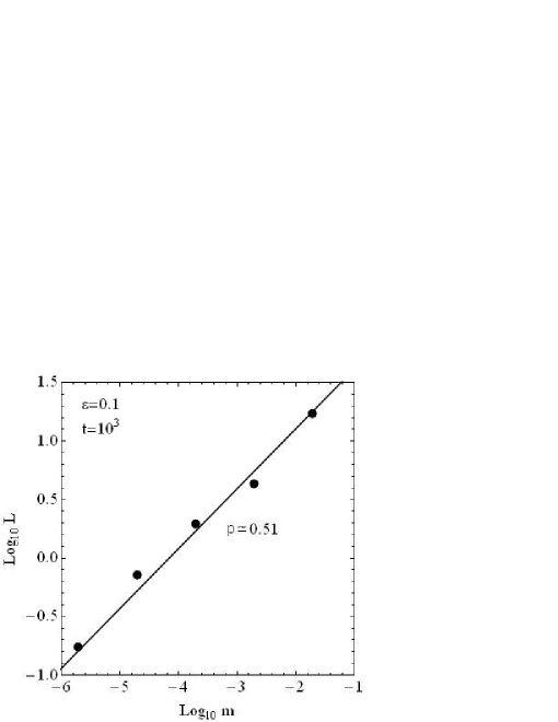
Figure 15: Logarithm of the mean Lyapunov number of the orbits in the ensembles of initial conditions as described in the text versus the central mass parameter $m=m_{bh}/m_{bar}$ (in logarithmic scale) in a disc-barred galaxy model. The logarithmic slope indicates a power-law exponent $p=0.51$.

Figure 15 shows the main result: the mean Lyapunov number $L$ of the chaotic orbits choosen as above is plotted against the mass parameter $m$, choosen here as the ratio $m=m_{bh}/m_{bar}$, since this ratio is relevant to a quantification of the rate of secular evolution of the bar. We observe again that the numerical data can be fitted by a power-law $L\propto m^{p}$, with $p=0.51$.

We now interpret the mechanisms of chaos and identify the families of orbits which are responsible for this behavior.

5.3 Interpretation

The mechanism by which a central black hole generates chaos in a disc-barred galaxy can be visualized with the help of phase portraits, obtained by means of a suitable surface of section. Here we employ the apocentric condition $\dot{r}=0$, $\ddot{r}<0$, in order to define the surface of section. We then plot the intersection points of all orbits with the above section as projected on the plane $(\theta,p_{\theta})$.

Figure 16 shows the surface of section portrait at the energies (Jacobi constant values) $E_{j}=-204000$ and $E_{j}=-195000$, without central black hole (Fig.16a,d), or with a black hole of mass $m_{bh}=10^{6}M_{\odot}$ (Fig.16b,e). The change of phase space structure is evident, namely the insertion of the central mass destroys many rotational KAM curves, corresponding to regular (quasi-periodic) orbits around the galactic center. Also, at the second energy level (lower panels), which corresponds to motion closer to corotation, a number of librational KAM curves around the 1:4 island of stability are destroyed. In fact, one can see that at both energy levels the orbits converted to chaotic are tube orbits around the 2:1 and 4:1 branches of the $x_{1}$ stable periodic orbit. The periodic orbits themselves at the corresponding energies are shown in Fig.16c and f respectively.

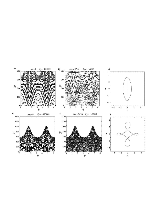
Figure 16: Apocentric Poincaré surfaces of section with $m_{bh}=0$ at the energies (a) $E_{J}=-204000$ and (d) $E_{J}=-195000$. (b,e) Same as in (a,d), but now with a central black hole of mass $m_{bh}=10^{6}M_{\odot}$. The $x_{1}$ periodic orbit (c) at the energy $E_{J}=-204000$ has a 2:1 form (two apocentric passages per revolution in the rotating frame), while (f) at the energy $E_{J}=-195000$ it has a 4:1 form.

The 2:1 orbits exist up to energies $\approx-199000$. When $m_{bh}=0$, the quasi-periodic tube orbits around a 2:1 orbit give rise to two islands of stability in the surface of section. The outermost librational invariant curves of these islands correspond to thick tube orbits (Fig.17). The crucial difference between the two tube orbits in Figs.17a and b is that in Fig.17a the tube orbit leaves a hole in the center, whose dimension is larger than the black hole’s sphere of influence. On the contrary, the tube thickness of the orbit in Fig.17b is larger than the half-width of the orbit’s amplitude of oscilation in the y-axis, i.e., the orbits leaves no hole in the center. Then, after the insertion of the central mass, the orbit with same initial conditions as in Fig.17a retains its regular (quasi-periodic) character (Fig.17c), while the orbit with same initial conditions as in Fig.17c becomes chaotic (Fig.17d). A similar criterion applies to whether or not a thick tube orbit around the 4:1 periodic orbit becomes regular or chaotic after the insertion of the central mass (Fig.17e-h). In fact, one readily finds that the initial conditions separating these two types of orbits correspond to the last librational KAM curve in the 4:1 island of stability of the section of Fig.16d.

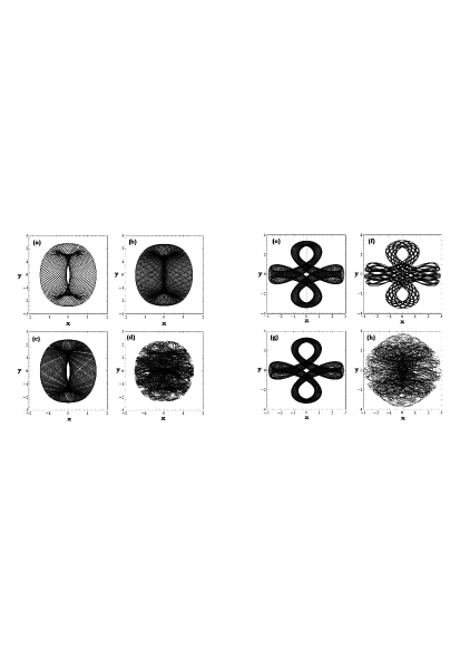
Figure 17: (a) Tube orbit with energy -216000 around the 2:1 periodic orbit before the insertion of the central mass. The initial conditions correspond to a librational invariant curve of the 2:1 island of stability which survives after the insertion of the black hole. (b) Same as in (a), but for initial conditions on an invariant curve of the 2:1 island of stability which is destroyed after the insertion of the black hole. (c) The orbit with same initial conditions as in (a) remains ordered after the insertion of a central mass $m_{bh}=10^{6}M_{\odot}$. (d) On the contrary, the orbit with same initial conditions as in (b) is converted to chaotic. (e,f) Same as in (a,b) but for two tube orbits of the 4:1 resonance. (g,h) The orbits with the same initial conditions as in (e,f) respectively, after the insertion of the central mass $m_{bh}=10^{6}M_{\odot}$. The one of (g) remains regular, while the one of (h) is chaotic.

Investigating the efficiency of the above mechanism to other resonances, one finds that the mechanism is not able to produce chaotic orbits in the cases of other low-order resonances like 3 : 1 and 6 : 1. In fact, the tube orbits trapped around these central periodic orbits in this model form rather small islands of stability. Thus, the tube thickness is small, and we find no tube orbits able to cross the central masses’ sphere of influence. A similar restriction holds for higher order families in the same model.

6 Conclusions

In the present paper we analyze the origin of a numerically observed approximate power-law relation $L\propto m^{p}$, with $p\sim$0.3–0.5, where $L$ is the mean Lyapunov exponent of centrophilic orbits in galaxies with central masses (black holes), and $m$ the mass parameter, i.e., the ratio of the central mass over the mass of the galaxy. Also, we find that such a law can be recovered in quite different contexts and models of galactic systems, ranging from elliptical galaxies with cores or cusps to rotating barred galaxies. In particular:

i) We first make numerical experiments with a simple model of elliptical galaxy with smooth central force field, to which the force field of the central mass is superposed. The experiments confirm the power-law $L\propto m^{p}$, when $L$ is estimated through its ‘finite time’ analog, i.e. the mean value of finite-time Lyapunov exponents. We demonstrate the statistics of these values for centrophilic orbits. We also find that $p$ has a tendency towards the upper limit 0.5 at longer integration times.

ii) We demonstrate that the law $L\propto m^{p}$ can be extracted also from compiling data of previous works in the literature (Merritt & Valluri (1996), Kandrup & Sideris (2002)), in galaxies with both smooth and cuspy centers.

iii) We make a theoretical analysis of the Lyapunov exponents for centrophilic box-like orbits in elliptical galaxies. We demonstrate that the mean Lyapunov exponent can be obtained by independently estimating a) the mean value of the so-called ‘stretching number’ (=one-step Lyapunov number) at every transit of an orbit from the sphere of influence of the central mass, and b) the rate of visits of the orbits to the sphere of influence. In both cases, we find how the various estimates depend on $m$ as well as on the orbital energy. Regarding (b), we find two different estimates, according to whether an orbit can be characterized as ‘planar’ or ‘3D’. Putting all estimates together, one arrives at a theoretical reproduction of the $L\propto m^{p}$ law.

iv) In the case of models with central cusps, we find a critical mass scale $m_{c}$, such that for central mass parameters $m<m_{c}$ the chaotic behavior of the centrophylic orbits is dominated by the central cusp (we call this ‘residual chaos’), while for $m>m_{c}$ an approximate power-law correlation $L\propto m^{p}$ is restored, with $p\approx 0.4$. The critical mass scale $m_{c}$ as well as the ‘residual mean Lyapunov exponent’ $L_{0}$ are increasing functions of the exponent $\gamma$ in power-law central cusps $\rho(r)\sim r^{-\gamma}$.

v) We finally explore numerically the correlation between $L$ and $m$ for the centrophylic orbits in disc galaxies with rotating bars. In this case, while there can be no box-like centrophilic orbits, we find several quasi-periodic tube orbits around the main families of periodic orbits (like 2:1 or 4:1), for which the tube is thick enough so as to pass arbitrarily close to the center. These orbits support the rising density profile of the bar at the center. Their initial conditions are close to the last librational KAM curve of the islands of stability around their corresponding periodic orbits. Numerically, we observe that only the tube orbits around the lowest-order periodic orbits can become centrophylic. Furthermore, for the chaotic counterparts of these orbits, after the insertion of the black hole, we numerically recover again a correlation of the form $L\propto m^{p}$.

Appendix

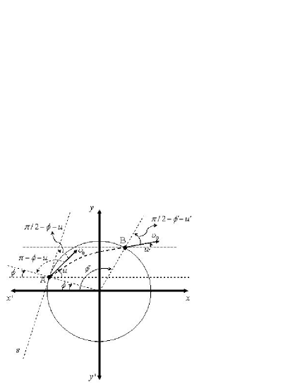
Figure 18: Schematic representation of our model for orbit transits via the sphere of influence of the central mass. An orbit enters the sphere at point A and exits at point B. Hyperbolic Keplerian dynamics is assumed in order to estimate the orbit’s local ‘stretching number’ arising at the transit (see text).

We theoretically estimate the local value of the ‘stretching number’ of an orbit transiting the sphere of influence of the central mass (Fig.18), schematic, as follows: approximating the motion during the transit as Keplerian, in polar co-ordinates $(r,\phi)$ with respect to the origin on a plane including the origin and the entry and exit points (A,B respectively), one has

$${1\over r}={{Gm\over C^{2}}+A\cos(\phi-\phi_{0})}$$ (39)

where $C$ is the local value of the angular momentum (assumed constant during the transit, see section 3). The constant $A$ is given by:

$$A=e{Gm\over C^{2}},$$ (40)

where $e=\sqrt{1+{2EC^{2}}/{mG^{2}}}$, whereas $\phi_{0}$ is the angle corresponding to the closest approach to the origin, at distance ($r_{min}$. The orbit has the the same velocity measure $v_{0}$ at the points A and B. We assume that the velocity vector at A forms an angle $u$ with the horizontal axis.

With the above conventions, to a given entry angle $\phi$ corresponds a given exit angle $\phi^{\prime}$ from the sphere of influence. After some algebra (taking into account Eq.(39) as well as the preservation of energy and angular momentum), we find:

$${\phi-\phi^{\prime}} = 2\cos^{-1}[{{\upsilon_{0}\sin{(\phi+u)}}\over{\sqrt{{({Gm/{{r_{m}\upsilon_{0}\sin{(\phi+u)}}}})}^{2}+\upsilon_{0}^{2}-{2Gm/{r_{m}}}}}}$$ (41)

$${({1-{Gm\over{{{r_{m}\upsilon_{0}^{2}\sin^{2}{(\phi+u)}}}}}})}]~{}~{}.$$

The local value of the stretching number can now be estimated by the difference in $\phi^{\prime}$ for two nearby orbits entering at slightly different angles $\phi$. Taking the derivative of eq.(41) we have:

$$|{d\phi^{\prime}\over{d\phi}}|=|1+{d\over{d\phi^{\prime}}}[2\cos^{-1} [ {{\upsilon_{0}\sin{(\phi+u)}}\over{\sqrt{{({Gm/{{r_{m}\upsilon_{0}\sin{(\phi+u)}}}})}^{2}+\upsilon_{0}^{2}-{2Gm/{r_{m}}}}}}$$ (42)

$${({1-{Gm\over{{{r_{m}\upsilon_{0}^{2}\sin^{2}{(\phi+u)}}}}}})}]]|~{}~{}.$$

Re-orienting the frame of reference, without loss of generality the parameter $u$ can be set equal to zero. The quantity $|{d\phi^{\prime}/{d\phi}}|$ is the measure of the stretching number $a$ for the transit. motion inside the sphere $r_{m}$. One can check that for typical energies of centrophilic orbits, one has $2mr_{m}\upsilon_{0}^{2}<<r_{m}^{2}\upsilon_{0}^{4}$. Then, Eq.(42) reduces to:

$$|{d\phi^{\prime}\over{d\phi}}|\simeq|{1-2{{1+{{m\csc^{2}\phi}/{r_{m}\upsilon_{0}^{2}}}}\over{1+{{m^{2}\csc^{2}\phi}/{r_{m}^{2}\upsilon_{0}^{4}}}}}}|~{}~{}.$$ (43)

The mean stretching number of a transit at given velocity $\upsilon_{0}$, with respect to all possible angles $\phi$ can be estimated by the integral of the quantity $\log|{d\phi^{\prime}/{d\phi}}|$ over all possible angles

$$\overline{\log\left|{d\phi^{\prime}\over{d\phi}}\right|} = {2\over{\pi}}\int_{0}^{\pi/2}\log|{d\phi^{\prime}\over{d\phi}}|d\phi=$$

$${2\over{\pi}}\int_{0}^{\pi/2}\log|{1-2{{1+{m\over{r_{m}\upsilon_{0}^{2}}}\csc^{2}\phi}\over{1+{m\over{r_{m}^{2}\upsilon_{0}^{4}}}\csc^{2}\phi}}}|d\phi={2\over{\pi}}\int_{0}^{\pi/2}\log|{(1-2{{\alpha_{0}+\sin^{2}\phi}\over{\alpha_{0}^{2}+\sin^{2}\phi}})|}d\phi=$$

$${2\over{\pi}}\int_{0}^{\pi/2}\log{(2{{\alpha_{0}+\sin^{2}\phi}\over{\alpha_{0}^{2}+\sin^{2}\phi}}-1)}d\phi=\log{(2{{1+\alpha_{0}}\over{1+\alpha_{0}^{2}}}-1)}+2\log{\sqrt{1+\alpha_{0}^{2}}(1+\sqrt{{\alpha_{0}(\alpha_{0}-2)}\over{\alpha_{0}^{2}-2\alpha_{0}-1}})\over{\alpha_{0}+\sqrt{1+\alpha_{0}^{2}}}}$$

where $\alpha_{0}=m/r_{m}\upsilon_{0}^{2}$. At mass ranges $10^{-5}<m<10^{-2}$ the value of $\alpha_{0}$ is in general a small quantity, except for small energies ($E<0.03$ in our units), which, however, can be readily checked to correspond to orbits residing always within the sphere $r=r_{m}$, i.e. pyramids (Merritt & Vasiliev (2011)). Excluding such orbits, we set $\alpha_{0}^{2}=0$ in the previous equation and obtain:

$$\overline{\log\left|{d\phi^{\prime}\over{d\phi}}\right|}\simeq\log{({1+2\alpha_{0}})}+2\log{(1+\sqrt{{-2\alpha_{0}}\over{-2\alpha_{0}-1}})\over{a+1}}$$

$$=\log{({1+2\alpha_{0}})}+2\log{(1+{{\sqrt{\alpha_{0}}}{\sqrt{{-2}\over{-2\alpha_{0}-1}}}})\over{a+1}}~{}~{}.$$ (45)

Expanding Eq.(Effective power-law dependence of Lyapunov exponents on the central mass in galaxies) with respect $a_{0}^{1/2}$ we find:

$$\overline{\log|{d\phi^{\prime}\over{d\phi}}}|\simeq 2{\alpha_{0}}+2\log{(1+{\sqrt{\alpha_{0}}{\sqrt{2}}})}=2{\alpha_{0}}+2{\sqrt{2}\sqrt{\alpha_{0}}}$$

$$={2\over{(r_{m}\upsilon_{0}^{2})}}m+{\sqrt{2}2\over{(r_{m}\upsilon_{0}^{2})^{1/2}}}\sqrt{m}\simeq{\sqrt{8\over{(r_{m}\upsilon_{0}^{2})}}}\sqrt{m}~{}~{}.$$ (46)

In Eq.(Effective power-law dependence of Lyapunov exponents on the central mass in galaxies) the quantity $r_{m}$ depends on $m$ ($r_{m}\propto m^{1/3}$). Furthermore in the limit of the sphere of black hole’s influence, energy is approximately equal with the kinetic energy ($\upsilon_{0}^{2}\propto E$), whereby the last expression can be written in the form:

$$\overline{a}\approx\overline{\log|{d\phi^{\prime}\over{d\phi}}}|\propto{m^{1/3}\over E^{1/2}}~{}$$ (47)

i.e. we arrive at the estimate of Eq.(17).

References

- Binney & Merrifield (1998) Binney, J., Merrifield, S., 1998, ‘Galactic Astronomy’, Princeton University Press.
- Binney & Tremaine (2008) Binney, J., Tremaine, S., 2008, ‘Galactic Dynamics’, 2nd edition, Princeton University Press.
- Contopoulos (1960) Contopoulos, G., 1960, Zeitschrift fur Astrophysik, 49, 273
- Contopoulos (1981) Contopoulos, G., 1981, Astron. Astrophys., 102, 265
- Contopoulos et al. (2002) Contopoulos, G., Voglis, N., Kalapotharakos, C., 2002, Cel. Mech. Dyn. Astron., 83, 191
- Dehnen (1993) Dehnen, W., 1993, Mon. Not. R. Astron. Soc., 265, 250.
- Debattista (2006) Debattista, V. P., 2006, New Horizons in Astronomy: Frank N. Bash Symposium, ASP Conference Series, 352
- Efthymiopoulos et al. (2004) Efthymiopoulos, C., Contopoulos, G., Giorgilli, A., 2004, J. Phys. A Math Gen, 37, 10831.
- Efthymiopoulos et al. (2007) Efthymiopoulos, C., Voglis, N., Kalapotharakos, C., 2007, Lect. Notes Phys. 729, 297
- Faber et al. (1997) Faber, S. M., Tremaine, S., Ajhar, E.A., Byun, Y., Dressler, A., Gebhardt, K., Grillmair, C., Kormendy, J., Lauer, T.R., Richstone, D., 1997, Astron. J., 114, 1771
- Ferrarese et al. (1994) Ferrarese, L.,van den Bosch, F.C., Ford, H.C., Jaffe, W., O’Connell, R.W., 1994, Astron. J., 108, 1598.
- Ferrarese & Ford (2005) Ferrarese, L., Ford, H.C., 2005, Space Sci. Rev., 116, 523
- Fridman & Merritt (1997) Fridman, T., Merritt, D., 1997, Astron. J., 114, 1479
- Friedli & Benz (1993) Friedli, D., Benz, W., 1993, Astron. Astrophys., 268, 65
- Friedli (1994) Friedli, D., 1994, in ‘Mass-Transfer Induced Activity in Galaxies’, I. Shlosman (ed), Cambridge University Press, p.268
- Froeschlé et al. (1997) Froeschlé, C., Lega, E., Gonczi, R., 1997, Cel. Mech. Dyn. Astron., 67, 41
- Fux (2001) Fux, R. 2001, Astron. Astrophys., 373, 511
- Gebhardt et al. (1996) Gebhardt, K., Richstone, D., Edward, A., Lauer, T.R., Byun, Y.I., Kormendy, J., Dressler, A., Faber, S.M., Grillmair, C., Tremaine, S., 1996, Astron. J., 112, 105
- Gebhardt et al. (2000) Gebhardt, K., Richstone, D., Kormendy, J., Lauer, T.R., Ajhar, E.A., Bender, R., Dressler, A., Faber, S.M., Grillmair, C., Magorrian, J., Tremaine, S., 2000, Astron. J., 119, 1157
- Gerhard & Binney (1985) Gerhard, O.E., Binney, J., 1985, Mon. Not. R. Astron. Soc., 216, 467
- Gültekin et al. (2009a) Gültekin, K., Richstone, D.O., Gebhardt, K., Lauer, T.R., Pinkney, J., Aller, M.C., Bender,R., Dressler, A., Faber, S.M., Filippenko, A.V., Green, R., Ho Luis C., Kormendy, J., Siopis, C., 2009, Astrophys. J., 695, 1577
- Gültekin et al. (2009b) Gültekin, K., Richstone, D., Gebhardt, K., Lauer, T.R., Tremaine, S., Aller, M.C., Bender, R., Dressler, A., Faber, S.M., Filippenko, A.V., Green R., Ho Luis, C., Kormendy, J., Magorrian, J., Pinkney, J., Siopis, C., 2009, Astrophys. J., 698, 198
- Hasan et al. (1993) Hasan, H., Pfenniger, D., Norman, C., 1993, Astrophys. J., 409, 91
- Holley-Bockelmann et al. (2001) Holley-Bockelmann, K., Mihos, J.C., Sigurdsson, S., Hernquist, L., 2001, Astrophys. J., 549, 149
- Holley-Bockelmann et al. (2002) Holley-Bockelmann, K., Mihos, J.C., Sigurdsson, S., Hernquist, L., Norman, C., 2002, Astrophys. J., 567, 817
- Jesseit et al. (2005) Jesseit, R., Naab, T., Burkert, A., 2005, Mon. Not. R. Astron. Soc., 360, 1185
- Kalapotharakos et al. (2004) Kalapotharakos, C., Voglis, N., Contopoulos, G., 2004, Astron. Astrophys., 428, 905
- Kalapotharakos & Voglis (2005) Kalapotharakos, C., Voglis, N., 2005, Cel. Mech. Dyn. Astron., 92, 157
- Kalapotharakos (2008) Kalapotharakos, C., 2008, Mon. Not. R. Astron. Soc., 389, 1709
- Kandrup & Sideris (2002) Kandrup, H., Sideris, I., 2002, Astrophys. J., 471, 82
- Kaufmann & Contopoulos (1996) Kaufmann, D.E., Contopoulos, G., 1996, Astron. Astrophys., 309, 381
- Kaufmann & Patsis (2005) Kaufmann, D.E., Patsis, P., 2005, Astrophys. J., 624, 693
- Kormendy et al. (1995) Kormendy, J., Richstone, D., 1995, Ann. Rev. Astron. Astrophys., 33, 581
- Kormendy et al. (1997) Kormendy, J., Bender, R., Magorrian, J., Tremaine, S., Gebhardt, K., Richstone, D., Dressler, A., Faber, S.M., Grillmair, C., Lauer, T.R., 1997, Astrophys. J., 482, L139
- Kormendy et al. (1998) Kormendy, J., Bender, R., Evans, A.S., Richstone, D., 1998, Astron. J., 115, 1823
- Kormendy & Ho (2013) Kormendy, J., Ho, L.C., 2013, Ann. Rev. Astron. Astrophys., 51, 511
- Lauer et al. (1995) Lauer, T.R., Ajhar, E.A., Byun, Y.I., Dressler, A., Faber, S.M., Grillmair, C., Kormendy, J., Richstone, D., Tremaine, S., 1995, Astron. J., 110, 2622
- McConell & Ma (2013) Merritt, D., 1999, Astr. Soc. Pacific Conf. Ser., 182, 164.
- Merritt (1999) Merritt, D., 1999, Astr. Soc. Pacific Conf. Ser., 182, 164.
- Merritt (2013) Merritt, D., 2013, ‘Dynamics and Evolution of Galactic Nuclei’, Princeton University Press
- Merritt & Fridman (1996) Merritt, D., Fridman, T., 1996, Astrophys. J., 460, 136
- Merritt & Quinlan (1998) Merritt, D., Quinlan, D., 1998, Astrophys. J., 498, 625
- Merritt & Valluri (1996) Merritt, D., Valluri, M., 1996, Astrophys. J., 471, 82
- Merritt & Valluri (1999) Merritt, D., Valluri, M., 1999, Astron. J., 118, 1177
- Merritt & Vasiliev (2011) Merritt, D., Vasiliev, E., 2011, Astrophys. J., 726, 61
- Miralda-Escudé & Schwarzschild (1989) Miralda-Escudé, J., and Schwarzschild, M., 1989, Astrophys. J., 339, 752.
- Muzzio et al. (2005) Muzzio, J.C., Carpintero, D., Wachlin, F.C., 2005, Cel. Mech. Dyn. Astron., 91, 173
- Muzzio (2006) Muzzio, J.C., 2006, Cel. Mech. Dyn. Astron., 96, 85
- Norman et al. (1996) Norman, C.A., Sellwood, J.A., Hasan, H., 1996, Astrophys. J., 462, 114
- Patsis et al. (1997) Patsis, P.A., Efthymiopoulos, C., Contopoulos, G., Voglis, N. 1997, Astron. Astrophys., 326, 493
- Pfenniger (1984) Pfenniger, D., 1984, Astron. Astrophys., 134, 373
- Pfenniger & de Zeeuw (1989) Pfenniger, D., de Zeeuw, T., 1989, in D. Merritt (ed.), ‘Dynamics of Dense Stellar Systems’, Cambridge University Press, p.81
- Pfenniger & Friedli (1991) Pfenniger, D., Friedli, D. 1991, Astron. Astrophys., 252, 75
- Pichardo et al. (2004) Pichardo, B., Martos, M., Moreno, E., 2004, Astrophys. J., 609, 144
- Shen & Sellwood (2004) Shen, J., Sellwood, J.A., 2004, Astrophys. J., 604, 614
- Sparke & Sellwood (1987) Sparke, L.S., Sellwood, J.A., 1987, Mon. Not. R. Astron. Soc., 225, 653
- van der Marel et al. (1997) van der Marel, R.P., de Zeeuw, P.T., Rix, H.W., 1997, Astrophys. J., 488, 119
- Valluri et al. (2010) Valluri, M., Debattista, V.P., Quinn, T., Moore, B., 2010, Mon. Not. R. Astron. Soc., 403, 525
- Vasiliev & Athanassoula (2012) Vasiliev, E., Athanassoula, E., 2012, Mon. Not. R. Astron. Soc., 419, 3268.
- Voglis & Contopoulos (1994) Voglis, N., Contopoulos G., 1994, J. Phys. A: Math. Gen., 27, 4899
- Young (1977) Young, P.J., 1977, Astrophys. J., 217, 287
- Young (1980) Young P., J., 1980, Astrophysical Journal, Part 1, 242, 1232-1237