Conductivity of strongly correlated bosons in optical lattices
in an Abelian synthetic magnetic field

Abstract

Topological phase engineering of neutral bosons loaded in an optical lattice opens a new window for manipulating of transport phenomena in such systems. Exploiting the Bose Hubbard model and using the magnetic Kubo formula proposed in this paper we show that the optical conductivity abruptly changes for different flux densities in the Mott phase. Especially, when the frequency of the applied field corresponds to the on-site boson interaction energy, we observe insulator or metallic behavior for a given Hofstadter spectrum. We also prove, that for different synthetic magnetic field configurations, the critical conductivity at the tip of the lobe is non-universal and depends on the energy minima of the spectrum. In the case of $1/2$ and $1/3$ flux per plaquette, our results are in good agreement with those of the previous Monte Carlo (MC) study. Moreover, we show that for half magnetic-flux through the cell the critical conductivity suddenly changes in the presence of a superlattice potential with uniaxial periodicity.

I Introduction

The Bose Hubbard model (BHM) is commonly used to describe many interesting physical systems e.g. superconductors with short coherence length Micnas et al. (1990), Josephson junction arrays Cha and Girvin (1994); van Otterlo et al. (1993) or quantum phase transitions in cold quantum gases Greiner et al. (2002); Stöferle et al. (2004) on which the idea of quantum simulations can be realized Jaksch and Zoller (2005). Recently, attention has been paid to the BHM behavior in a strong synthetic magnetic field Saha et al. (2010); Powell et al. (2010); Zaleski and Polak (2011); Powell et al. (2011); Sinha and Sengupta (2011); Nakano et al. (2012); Polak and Zaleski (2013); Struck et al. (2013) as well as to its transport properties Šmakov and Sø rensen (2005); Bhaseen et al. (2007, 2009); Lindner and Auerbach (2010); Tokuno and Giamarchi (2011); Chen et al. (2013); Kessler and Marquardt (2013). This research has opened the possibility of highly controllable BHM dynamics with explicitly designed kinetics which is a subject of our study.

Despite of the Josephson junction arrays van der Zant et al. (1992); van der Zant H. S. et al. (1996) up to now a strong magnetic field regime has been available by simulating a vector potential imposed on many body wave function of ultra-cold neutral gases. It has been realized by engineering the adequate phase of atoms when they change their quantum states upon hopping through the lattice sites, using e.g. Raman- and photo-assisted tunneling Lin et al. (2009); Aidelsburger et al. (2011); Aidelsburger et al. (2013a); Miyake et al. (2013), shaking of the lattice Struck et al. (2011, 2013). In particular, staggered Aidelsburger et al. (2011) and uniform Aidelsburger et al. (2013a); Miyake et al. (2013) magnetic field have been created. Such synthetic magnetic field has also been proposed to be generated by combining quadrupolar potential and modulation of tunneling in time Sø rensen et al. (2005), although it has not been realized yet (see also Jaksch and Zoller (2003)). Moreover, the relevant gauge degrees of freedom can be precisely experimentally verifiable and can cause interesting effects like finite momentum condensate Polak and Zaleski (2013). As follows from the above, the possibility of simulating a vector potential provides many opportunities which has made it a rapidly expanding area of research. The interest in the simulation has been growing in view of possible future application of ultra-cold quantum gases in topological quantum computation or spintronics Nayak et al. (2008); Hasan and Kane (2010).

If we consider the BHM equipped with orbital effects, its complexity considerably increases, as it develops a multi-subband structure dependent on the quantity of flux per plaquette. To the best of our knowledge the conductivity in a strong magnetic field has been considered mainly numerically in just a few papers. One of the main problems in carrying out the related calculations is the complex hopping term (Peierls factor) which occurs in the BHM Hamiltonian. This is the reason why the optical conductivity (OC) has been rarely studied. Y. Nishiyama Nishiyama (2001) has analyzed OC in the hard-core limit of the BHM with disorder. OC in Josephson junction arrays has been also studied within Landau levels framework without commensurability effects of magnetic field van Otterlo et al. (1993); Wagenblast et al. (1997). The critical conductivity could be much easier available in numerical calculations thanks to the correspondence between the BHM at integer filling and the XY model Cha and Girvin (1994); Kim and Stroud (2008) in which the cases $f=1/2$ and $f=1/3$ flux per plaquette has been studied Cha and Girvin (1994). Using this correspondence E. Granato and J. Kosterlitz Granato and Kosterlitz (1990) derived analytically the value of critical conductivity for half flux per plaquette. Also Y. Nishiyama Nishiyama (2001) by applying the exact diagonalization method has shown that the critical conductivity subjected to magnetic field is non-universal. Understanding of such a non-universal behavior gives better insight into physics behind the superconductor-insulator phase transition phenomena.

The engineering of the conductivity can be also improved by changing experimentally the value of potential on adjacent sites. This solution has been recently of growing interest because it allows a simple experimental realization Aidelsburger et al. (2011); Aidelsburger et al. (2013b) and generates interesting physical phenomena Delplace and Montambaux (2010); Polak and Zaleski (2013). In particular, tuning the uniaxially periodic potential with a magnetic-flux quantum per unit cell results in a new possibility of merging cones simulation in which semi-Dirac point in the Hofstadter spectrum emerges Delplace and Montambaux (2010). Recently this possibility has been also exploited in the context of time-of-light patterns with and without synthetic magnetic field Polak and Zaleski (2013).

In this work we present a theory of conductivity valid in a strong magnetic field in which only intra-Hofstadter-band transitions are taken into account. In the Mott phase for the square lattice, we describe the optical behavior using two exemplary values of uniform magnetic field: $f=1/2$ and $f=1/4$ as well as the case with uniaxially staggered potential. We highlight the fact that the calculation could be straightforwardly extended to an arbitrary amplitude of the magnetic field and also gauge degree of freedom. For verification of the results obtained, a combination of two types of currently available experiments is proposed. Our method is tested for the the critical value of conductivity on the Mott insulator - superfluid phase boundary in two dimensions (2D). The proposed analytical approach correctly reproduces critical conductivity in the absence of magnetic field $f=0$ (first calculated in Fisher et al. (1990)), $f=1/2$ (MC numerical solution in Ref. Cha and Girvin (1994) and analytic one Granato and Kosterlitz (1990); Grason and Bruinsma (2006) but using a model corresponding to BHM), $f=1/3$ (only numerical solution in Ref. Cha and Girvin (1994) based on MC). We have also extended the calculations of critical conductivity over the range of arbitrary $f=p/q$ which has not been hitherto reported literature and confirmed its non-universal behavior upon changes in the amplitude of magnetic field. The influence of uniaxially staggered potential is also discussed. We compare our results with presently available numerical and experimental data.

The paper is organized as follows. The BHM in the strong uniform magnetic field is reviewed in Sec. II. In Sec. III we apply our method to study the optical conductivity and its critical value for different strengths of synthetic magnetic fields, taking into consideration the effects of uniaxially staggered potential. In the last section we give a short summary of our results.

II Model

The BHM Hamiltonian in standard notation is given by

$$H=-\sum_{\langle ij\rangle}\tilde{J}_{ij}\left(\hat{b}_{i}^{\dagger}\hat{b}_{j}+\textrm{H.c.}\right)+\frac{U}{2}\sum_{i}\hat{n}_{i}\left(\hat{n}_{i}-1\right)-\mu\sum_{i}\hat{n}_{i}$$ (1)

where $\hat{b}_{i}$ ($\hat{b}_{i}^{\dagger}$) is an operator which annihilate (create) boson on site $i$ and $\hat{n}_{i}=\hat{b}_{i}^{\dagger}\hat{b}_{i}$. $U$ and $\mu$ are on-site boson interaction and chemical potential, respectively. Hopping integral is denoted by $\tilde{J}_{ij}$ and has a form

$$\tilde{J}_{ij}=J_{ij}e^{i\frac{e^{*}}{\hbar c}\int_{j}^{i}\mathbf{A}_{0}\cdot d\mathbf{l}}$$ (2)

with non-zero isotropic factor $J_{ij}=J$ in respect to adjacent sites. Magnetic field $B$ is introduced by a vector potential $\mathbf{A}_{0}=B(0,x,0)$ which is taken in the Landau gauge. Further in our calculation we define $Ba^{2}e^{*}/\hbar c=2\pi f$ where $f=Ba^{2}e^{*}/hc=p/q$ is a flux per plaquette ($p$ and $q$ are coprime integers). $f$ depends on the charge of the boson $e^{*}$, lattice spacing $a$, Planck constant $h$ and speed of light $c$. It is important to stress that in an optical lattice the quantities like $B$ and $e^{*}$ are effectively created through tunability of the $p/q$ ratio.

Using the coherent state path integral for the BHM hamiltonian (Eq. (1)), the partition function can be written as follows

$$\mathcal{Z}\left[\mathbf{A}_{0}\right]=\int\mathcal{D}b^{*}\mathcal{D}b\,e^{-\left(S_{0}+S_{1}\left[\mathbf{A}_{0}\right]\right)/\hbar},$$ (3)

$$S_{0} = \sum_{i}\int_{{}_{0}}^{\hbar\beta}d\tau\left\{b_{i}^{*}(\tau)\hbar\frac{\partial}{\partial\tau}b_{i}(\tau)\right.$$

$$\left.+\frac{U}{2}b_{i}^{*}(\tau)b_{i}^{*}(\tau)b_{i}(\tau)b_{i}(\tau)-\mu b_{i}^{*}(\tau)b_{i}(\tau)\right\},$$

$$S_{1}\left[\mathbf{A}_{0}\right]=-\sum_{\langle ij\rangle}\int_{{}_{0}}^{\hbar\beta}d\tau\;J_{ij}e^{i\frac{e^{*}}{\hbar c}\int_{j}^{i}\mathbf{A}_{0}\cdot d\mathbf{l}}\left(b_{i}^{*}(\tau)b_{j}(\tau)+\textrm{c.c.}\right),$$ (5)

where the integrals in Eq. (II) and Eq. (5) are taken over imaginary time $\tau$ and $\beta=1/k_{B}T$.

To take into account magnetic field in the strong coupling limit of BHM we follow the same procedure as in Refs. Sengupta and Dupuis (2005); Sinha and Sengupta (2011) i.e. we perform the double Hubbard-Stratonovich transformation together with cumulant expansion. In the following, we focus on the Mott phase and we approximate effective action to second order in the $\mathcal{B}_{\mathbf{k}n}^{q}$ , $\left(\mathcal{B}_{\mathbf{k}n}^{q}\right)^{\dagger}$ fields

$$S^{eff}=\sum_{\mathbf{k}n}\left(\mathcal{B}_{\mathbf{k}n}^{q}\right)^{\dagger}\left[-\hbar G_{0}^{-1}(i\omega_{n})\mathbf{I}+\mathbf{J}^{q}(\mathbf{k})\right]\mathcal{B}_{\mathbf{k}n}^{q},$$ (6)

where $\mathbf{I}$ is an identity matrix and

$$\mathcal{B}_{\mathbf{k}n}^{q}=\left(b_{\mathbf{k},n},\;b_{\mathbf{k}+\mathbf{p},n},,\;...,\;b_{\mathbf{k}+(q-1)\mathbf{p},n}\right)^{T},$$ (7)

with $\mathbf{p}=(2\pi f,\;0)$ and $\omega_{n}=2\pi n/\hbar\beta$ is the Matsubara frequency ($n$ is an integer number). In Eq. (6) the summation is performed over wave vectors $\mathbf{k}$ within the first magnetic Brillouin zone where $\left|k_{x}\right|\leqslant\pi/qa$ and $\left|k_{y}\right|\leqslant\pi/a$. $G_{0}(i\omega_{n})$ is the on-site Green function (i.e. is local where $J=0$) and at the zero temperature limit it has the form

$$\frac{1}{\hbar}G_{0}(i\omega_{n})=\frac{n_{0}+1}{i\hbar\omega_{n}+E_{n_{0}}-E_{n_{0}+1}}-\frac{n_{0}}{i\hbar\omega_{n}+E_{n_{0}-1}-E_{n_{0}}}$$ (8)

with on-site energy $E_{n_{0}}=-\mu n_{0}+Un_{0}(n_{0}-1)/2$. $n_{0}$ is the integer number obtained from the on-site energy minimization for a given chemical potential $\mu$. The last object in (6) that requires explanation is $\mathbf{J}^{q}(\mathbf{k})$. It represents a non-diagonal $q\times q$ matrix similar to that obtained earlier Hasegawa et al. (1989)

$$\mathbf{J}^{q}(\mathbf{k})/J=\begin{bmatrix}M_{0}&-e^{ik_{y}a}&&&-e^{-ik_{y}a}\\ -e^{-ik_{y}a}&M_{1}&\ddots&0\\ &\ddots&\ddots&\ddots\\ &0&\ddots&M_{q-2}&-e^{ik_{y}a}\\ -e^{ik_{y}a}&&&-e^{-ik_{y}a}&M_{q-1}\end{bmatrix},$$ (9)

where $M_{\alpha}=-2\cos(k_{x}a+2\pi\alpha f)$. The set of eigenvalues of the matrix (9) leads to the Hofstadter spectrum Hofstadter (1976).

It is important to comment here on the notation used above. Although $b,\;b^{*}$ fields introduced in Eq. (6) have identical notation as in Eq. (3) they are not the same. Namely, those fields in which the quadratic effective action Eq. (6) is evaluated, were introduced during the second Hubbard-Stratonovich transformation mentioned above. However, both kind of fields have the same correlation function Sengupta and Dupuis (2005) and for this reason we treat them on an equal footing.

For the effective action in Eq. (6) we can find a unitary matrix $U_{q}(\mathbf{k})$ Saha et al. (2010) that diagonalizes it, i.e.

$$S^{eff}=-\sum_{\mathbf{k}n}\left(\tilde{\mathcal{B}}_{\mathbf{k}n}^{q}\right)^{\dagger}\left[\mathcal{G}^{d}(\mathbf{k},\,i\omega_{n})\right]^{-1}\tilde{\mathcal{B}}_{\mathbf{k}n}^{q}\;,$$ (10)

where $\mathcal{G}^{d}(\mathbf{k},\,i\omega_{n})=U_{q}(\mathbf{k})\left[\hbar G_{0}^{-1}(i\omega_{n})\mathbf{I}-\mathbf{J}^{q}(\mathbf{k})\right]^{-1}U_{q}^{\dagger}(\mathbf{k})$ is an inverse of diagonal Green function and $\tilde{\mathcal{B}}_{\mathbf{k}n}^{q}=U_{q}(\mathbf{k})\mathcal{B}_{\mathbf{k}n}^{q}$. As shown in Sec. III this diagonal form of $\mathcal{G}^{d}(\mathbf{k},\,i\omega_{n})$ has q-bands which are labeled by $\alpha$ number.

The above denotations will be useful for further study. In order to simplify the calculations we also set the lattice constant $a$ and the reduced Planck constant $\hbar$ to unity.

III Conductivity in magnetic field

To construct a correct theory of optical conductivity in the strong magnetic field described by the BHM, we should go beyond the linear response regime. This situation is more complicated than that previously studied (e.g., see Ref. Kampf and Zimanyi (1993)) due to the presence of a synthetic magnetic field $\mathbf{A}_{0}$ which significantly modifies the single-particle spectrum. This modification implies that the commensurability field effects become important. As a consequence, the amplitude of hopping term is a complex number (Eq. (5)) and the boson field is described by more than one component (Eq. (7)). To overcome these difficulties in calculation of the transport properties we assume that such an initial state will be subtly affected by an additional field $\left|\mathbf{A}\right|\ll\left|\mathbf{A_{0}}\right|$, which is responsible for generation of optical conductivity in the linear response regime. Therefore, if we want to study the response of the system to a strong magnetic field, we simply add to the $\mathbf{A}_{0}$ some small perturbation of this field in the form of a vector potential $\mathbf{A}$ i.e.

$$\int_{\mathbf{r}_{i}}^{\mathbf{r}_{j}}\mathbf{A}_{0}\cdot d\mathbf{l}\rightarrow\int_{\mathbf{r}_{i}}^{\mathbf{r}_{j}}\mathbf{A}_{0}\cdot d\mathbf{l}+\int_{\mathbf{r}_{i}}^{\mathbf{r}_{j}}\mathbf{A}\cdot d\mathbf{l}$$ (11)

and use the linear response theory as a starting point with respect to the quantity $\mathbf{A}$. This leads to the well known expression for the optical conductivity (e.g., see Refs. Wu and Phillips (2006); Kampf and Zimanyi (1993); Cha et al. (1991))

$$\sigma_{xx}^{\mathbf{A}_{0}}(i\omega)=-\left.\frac{1}{N\omega}\sum_{ij}\int_{0}^{\beta}d\tau e^{i\omega\tau}\frac{\delta^{2}\ln\mathcal{Z}\left[\mathbf{A}^{\prime}\right]}{\delta A_{i}^{x}(\tau)\delta A_{j}^{x}(0)}\right|_{\mathbf{A}=0},$$ (12)

but in our case the conductivity depends upon vector potential $\mathbf{A}_{0}$ and consequently on magnetic field and in this dependence the commensurability effects are included.

Performing the calculations in Eq. (12) we first go to the wave vector representation which allows proper incorporation of the perturbing vector potential $\mathbf{A}$, through the substitution $k_{x}\rightarrow k_{x}+\frac{e^{*}}{\hbar c}\mathbf{A}$ (we assume that $\mathbf{A}$ does not depend on position) and then we evaluate the derivatives in Eq. (12) getting

$$\sigma_{xx}^{\mathbf{A}_{0}}(i\omega)=-\frac{\left(e^{*}\right)^{2}}{\omega}\left\langle e_{kin}^{x}\right\rangle+\frac{1}{\omega}\Pi_{xx}(i\omega)\;,$$ (13)

where functional averages are taken with the partition function from Eq. (3). $e_{kin}^{x}$ and $\Pi_{xx}(\omega)$ are a kinetic and current-current correlation function, respectively (we set $c=1$). With the effective action from Eq. (10) we can evaluate Eq. (13) to the form

$$\Pi_{xx}(i\omega)=-\frac{1}{N}\sum_{\mathbf{kk^{\prime}}}\int_{0}^{\beta}d\tau\;e^{i\omega\tau}\left\langle j_{\mathbf{k}}^{x}(\tau)j_{\mathbf{k^{\prime}}}^{x}(0)\right\rangle,$$ (14)

$$e_{kin}^{x}=-\frac{1}{N}\sum_{\mathbf{k}}\sum_{\alpha=0}^{q-1}\left[\partial_{k_{x}}^{2}\epsilon_{q}^{\alpha}(\mathbf{k};p)\right]b_{\mathbf{k}+\alpha\mathbf{p}}^{*}(0)b_{\mathbf{k}+\alpha\mathbf{p}}(0),$$ (15)

$$j_{\mathbf{k}}^{x}(\tau)=e^{*}\sum_{\alpha=0}^{q-1}\left[\partial_{k_{x}}\epsilon_{q}^{\alpha}(\mathbf{k};p)\right]b_{\mathbf{k}+\alpha\mathbf{p}}^{*}(\tau)b_{\mathbf{k}+\alpha\mathbf{p}}(\tau),$$ (16)

where $\epsilon_{q}^{\alpha}(\mathbf{k};p)$ is an eigenvalue of $J_{q}(\mathbf{k})$ matrix defined in Eq. (9) and the current is given by Eq. (16). Eq. (13) is the Kubo formula valid in strong magnetic field (MKF) in which only intra-Hofstadter-band transitions are taken into account. This method, in contrast to that presented in Ref. van Otterlo et al. (1993) (see also Refs. Wagenblast et al. (1996, 1997); Dalidovich and Phillips (2001, 2002); Wu and Phillips (2006)), takes into account the commensurability effects of the magnetic field and covers the whole range of $\mathbf{k}$ and $\omega$ dependence.

For the simplest case, if we take the usual square lattice dispersion relation in the absence of magnetic field $\epsilon_{1}^{\alpha}(\mathbf{k};0)=-2J\left(\cos k_{x}+\cos k_{y}\right)$, one gets from Eq. (13)

$$\sigma_{xx}^{\mathbf{A}_{0}}(i\omega) = \frac{\left(e^{*}\right)^{2}J}{\omega}\frac{1}{N}\sum_{\mathbf{k}}2\cos k_{x}\left\langle b_{\mathbf{k}}^{*}(0)b_{\mathbf{k}}(0)\right\rangle$$

$$-\frac{4\left(e^{*}\right)^{2}J^{2}}{\omega}\frac{1}{N}\sum_{\mathbf{k},\mathbf{k}^{\prime}}\int_{0}^{\beta}d\tau\,\mathrm{e}^{i\omega\tau}\times$$

$$\sin(k_{x})\sin(k^{\prime}_{x})\langle b_{\mathbf{k}}^{*}(\tau)b_{\mathbf{k}}(\tau)b_{\mathbf{k}^{\prime}}^{*}(0)b_{\mathbf{k}^{\prime}}(0)\rangle\;,$$

which recovers a well known result Kampf and Zimanyi (1993).

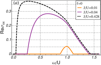
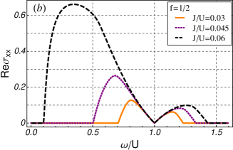
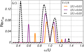
Figure 1: Real part of optical conductivity in the two-dimensional square lattice in Mott phase (first lobe) is sketched in $\sigma_{Q}$ units ($\sigma_{Q}=\left(e^{*}\right)^{2}/h$ is a quantum conductance). From the top - $f=0$ (a), $f=1/2$ (b), $f=1/4$ (c). Conductivity is plotted at zero temperature for different value of $J/U$ within the first lobe.

III.1 Optical conductivity in the BHM

III.1.1 The uniform field

Now we are interested in the OC in the Mott insulator phase. Using the fact that within the action (10) the four point correlation function in Eq (14) is factorized, we can rewrite Eq (13) to the form

$$\sigma_{xx}^{\mathbf{A}_{0}}(i\omega) = -\frac{\left(e^{*}\right)^{2}J}{\omega}\frac{1}{\beta N}\sum_{\mathbf{k}n}\sum_{\alpha=0}^{q-1}\partial_{k_{x}}^{2}\epsilon_{q}^{\alpha}(\mathbf{k};p)\mathcal{G}_{\alpha\alpha}^{d}(\mathbf{k},i\omega_{n})$$

$$-\frac{\left(e^{*}\right)^{2}}{\omega}\frac{1}{\beta N}\sum_{\mathbf{k}n}\sum_{\alpha=0}^{q-1}\times$$

$$\left[\partial_{k_{x}}\epsilon_{q}^{\alpha}(\mathbf{k};p)\right]^{2}\mathcal{G}_{\alpha\alpha}^{d}(\mathbf{k},i\omega_{n})\mathcal{G}_{\alpha\alpha}^{d}(\mathbf{k},i\omega_{n}+i\omega).$$

Mott insulator Green’s function is

$$\mathcal{G}_{\alpha\alpha}^{d}(\mathbf{k},i\omega_{n}) = \frac{G_{0}(i\omega_{n})}{1-\epsilon_{q}^{\alpha}(\mathbf{k};p)G_{0}(i\omega_{n})}$$

$$= \frac{z_{q}^{\alpha}(\mathbf{k};p)}{i\omega_{n}-E_{q}^{\alpha+}(\mathbf{k};p)}+\frac{1-z_{q}^{\alpha}(\mathbf{k};p)}{i\omega_{n}-E_{q}^{\alpha-}(\mathbf{k};p)}\,,$$

where the weight and dispersion of quasiparticles have the form

$$z_{q}^{\alpha}(\mathbf{k};p)=\frac{E_{q}^{\alpha+}(\mathbf{k};p)+\mu+U}{E_{q}^{\alpha+}(\mathbf{k};p)-E_{q}^{\alpha-}(\mathbf{k};p)}\;,$$ (20)

$$E_{q}^{\alpha\pm}(\mathbf{k};p)=\frac{\epsilon_{q}^{\alpha}(\mathbf{k};p)}{2}-\mu+U\left(n_{0}-\frac{1}{2}\right)\pm\frac{1}{2}\Delta_{q}^{\alpha}(\mathbf{k};p)$$ (21)

$$\Delta_{q}^{\alpha}(\mathbf{k};p)=\sqrt{\left[\epsilon_{q}^{\alpha}(\mathbf{k};p)\right]^{2}+4\epsilon_{q}^{\alpha}(\mathbf{k};p)U\left(n_{0}+\frac{1}{2}\right)+U^{2}}$$ (22)

In the following we are interested in the real and regular part of optical conductivity given by

$$\textrm{Re}\sigma_{xx}^{\mathbf{A}_{0}}(\omega)=\left(e^{*}\right)^{2}\frac{2\pi}{N}\sum_{\alpha=0}^{q-1}\sum_{\mathbf{k}}\left(\partial_{k_{x}}\epsilon_{q}^{\alpha}(\mathbf{k};p)\right)^{2}$$ (23)

$$\times\left\{n_{B}\left[E_{q}^{\alpha-}(\mathbf{k};p)\right]-n_{B}\left[E_{q}^{\alpha+}(\mathbf{k};p)\right]\right\}$$

$$\times\left[1-z_{q}^{\alpha}(\mathbf{k};p)\right]z_{q}^{\alpha}(\mathbf{k};p)\delta\left(\omega^{2}-\left(\Delta_{q}^{\alpha}(\mathbf{k};p)\right)^{2}\right)\;,$$

which has been obtained by evaluating Matsubara sum in Eq. (III.1.1) and performing standard analytical continuation $i\omega\rightarrow\omega+i\delta$ . The symbol $\delta(x)$ is a Dirac delta function and $n_{B}(x)$ is Bose-Einstein distribution function. Using density of states and taking zero-temperature limit, equation (23) can be rewritten as follows

$$\textrm{Re}\sigma_{xx}^{\mathbf{A}_{0}}(\omega)_{\textrm{}} = 2\pi^{2}\sigma_{Q}\sum_{\alpha}\sum_{s=\{+,-\}}\Xi_{q}^{\alpha}\left[u^{s}(\omega);p\right]\;,$$ (24)

$$\Xi_{q}^{\alpha}\left[v;p\right] = \rho_{q}^{\alpha}(v;p)\frac{J\left[z_{q}^{\alpha}(v;p)-1\right]z_{q}^{\alpha}(v;p)}{U\sqrt{4n_{0}\left(n_{0}+1\right)+\left(\omega/U\right)^{2}}}\;,$$ (25)

$$u^{\pm}(\omega) = \frac{U}{J}\left(2n_{0}+1\right)\left(1\mp\sqrt{1-\frac{1-\left(\omega/U\right)^{2}}{\left(2n_{0}+1\right)^{2}}}\right)\;,$$ (26)

where the density of states is given by

$$\rho_{q}^{\alpha}(v;p)=\frac{1}{N}\sum_{\mathbf{k}}\left[\partial_{k_{x}}\epsilon_{q}^{\alpha}(\mathbf{k};p)\right]^{2}\delta\left(v-\epsilon_{q}^{\alpha}(\mathbf{k};p)\right)\;.$$ (27)

For magnetic fields considered here (i.e. $f=0,\;1/2,\ 1/4$) the exact calculations of density of states in 2D was possible in terms of complete elliptic integrals (see Appendix V.1).

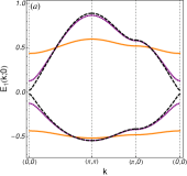
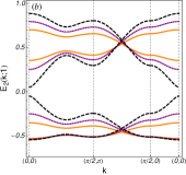
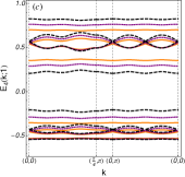
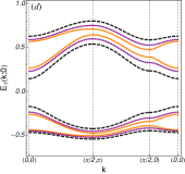
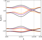
Figure 2: The wave vector $\mathbf{k}$ dependence of the quasi-particle energy dispersions $E_{q}^{\alpha\pm}(\mathbf{k};p)$ for different amplitudes of uniform magnetic field $f$ and staggered potential $\Delta$ in the first magnetic Brillouin zone. Plots $a$, $b$, $c$ correspond to the Figure 1 $a$, $b$, $c$, respectively. Additionally, plots $d$ and $e$ correspond to Fig. 4 and Fig. 5, respectively. This correspondence is revealed when choosing the same physical parameters for the same plotting style in the relevant figures.

In Fig. 1 we show the real part of OC at zero temperature in the Mott phase for different values of synthetic magnetic field. It is worth noting that its behavior reflects the tight binding dispersion of the lattice. As expected the OC is gradually broadened at the cost of vanishing gap when $J/U$ increases. Interestingly, for $f=1/4$, the contribution of the lowest frequency peak becomes much more significant when the $J/U$ ratio is tuned up.

For $\omega=U$, we observe that the existence of conductivity at this point directly depends on the spectrum weight value of the tight binding dispersion $\epsilon_{q}^{\alpha}(\mathbf{k};p)$. In particular, if the spectrum weight of $\epsilon_{q}^{\alpha}(\mathbf{k};p)$ at the center of the band is zero the conductivity also disappears. Such a situation for $\omega=U$ is satisfied when $f=1/2,\;1/4$ (even $q$) but for odd $q$ we should observe metallic behavior. This special behavior of OC at this point is directly related to the Dirac cones appearing in quasi-particle energy dispersion $E_{q}^{\alpha\pm}(\mathbf{k};p)$. The corresponding dispersions are plotted in Fig. 2 $a-c$ for the relevant set of parameters. In the Sec. III.2 we suggest an experiment to check this conjecture explicitly, because the quantities like the on-site interaction strength $U$ and boson hopping amplitude $J$ are fully controllable parameters in ultra-cold gases loaded on optical lattice.

Within the above framework we can also probe the critical value of conductivity at the tip of the lobe (for determination of the critical value of $\mu/U$ and $J/U$ see Ref. Sinha and Sengupta (2011)). For this range of parameters the OC is as shown in Fig. 3. The critical value of conductivity for $f=1/2$ ($1/4$) when $\omega\rightarrow 0$ is two (four) times higher than the value with magnetic field absent. These results are in agreement with those derived in Sec. III.3.

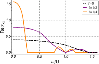
Figure 3: Optical conductivity for different values of magnetic field. The parameters $\mu/U$ and $J/U$ are chosen on the phase boundary where Mott insulator - superfluid phase transition takes a place. The plot shows that the critical value of conductivity for the $f=1/2$ ($1/4$) when $\omega\rightarrow 0$ is two (four) times higher than in the case when magnetic field is absent. $\textrm{Re}\sigma_{xx}$ was plotted in $\sigma_{Q}$ units.

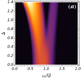
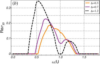
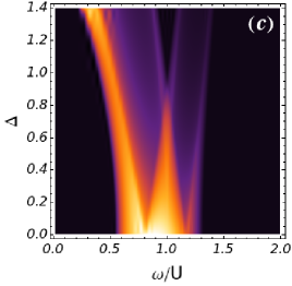
Figure 4: First (second) panel shows $yy$ ($xx$) component of the real part of the optical conductivity for different values of $\Delta$ in the absence of magnetic field. On the density sketch the lighter color indicates higher amplitude of the conductivity (black area correspond to the insulator behavior). All zero-temperature plots show the situation where the uniaxially staggered field is subjected to the $x$ axis. The ratio of hopping amplitude and on-site interaction energy is $J/U=0.03$ and the conductivity was plotted in $\sigma_{Q}$ units.

III.1.2 The uniform field with staggered potential

In the following we use the proposed framework of OC (see Eq. (13)) to study the transport phenomena under the influence of uniaxially staggered potential. The situations with the synthetic magnetic field absent ($f=0$) and with its value described by half flux per plaquette ($f=1/2$) are considered. The latter special case is a subject of current interest Delplace and Montambaux (2010). In both cases of OC i.e. $f=0$ and $f=1/2$ the staggered potential is controlled by the parameter $\Delta$ Polak and Zaleski (2013), which is included in the Hamiltonian (1) by an additional term in the form

$$\sum_{i_{x}i_{y}}(-1)^{i_{x}}\tilde{\Delta}\hat{b}_{i_{x}i_{y}}^{\dagger}\hat{b}_{i_{x}i_{y}}\;,$$ (28)

where $\Delta=\tilde{\Delta}/2J$ and $i_{x},\;i_{y}$ enumerate the positions of lattice sites along the $x$ and $y$ axis, respectively.

Fig. 4 and 5 show the frequency dependence of OC for $f=0$ and $f=1/2$, respectively. We are interested in $\sigma_{xx}^{\mathbf{A}_{0}}(\omega)$ and $\sigma_{yy}^{\mathbf{A}_{0}}(\omega)$ component in which the potential from site to site is varied in the $x$ direction (to see the expressions used in the calculations of OC see Appendix V.2).

The data presented in Fig. 4 and 5 imply a similar behavior of OC when $\Delta$ parameter is alternated. For example, on the basis of the staggered potential values with respect to its value for $\Delta=0$, we conclude that it has greater impact on the $xx$ component of OC than on $yy$ one. Besides the qualitative difference, we also observe a smaller amplitude of the OC in direction $x$ than in that perpendicular to $x$ within $xy$ plane. This behavior could be simply attributed to the variation in the potential in this particular direction (i.e. $x$). While the $yy$ component of the OC does not exhibit any special difference along $y$ axis (for chosen strip of sites the $\Delta$ is constant). Moreover, we show that the increase in $\Delta$ causes broadening a frequency dependence of OC.

In agreement with the conclusion drawn in Sec. III.1.1 the insulator behavior of the OC for $\omega=U$ (Fig. 5) is still maintained for $f=1/2$. In contrast to the situation with no magnetic field (see Fig.4) the gap naturally arises when the $\Delta$ parameter exceeds one (the single-particle spectrum also exhibits a similar behavior). This gap-like behavior is indeed observed in the quasi-particle energy dispersion $E_{q}^{\alpha\pm}(\mathbf{k};p)$ presented in Fig. 2 $d$ and $e$. Interestingly, the weight of the OC close to $\omega=U$ for $f=1/2$ is greater than for $f=0$.

It is worth noting that the complex behavior of the OC in the direction of applied uniaxially staggered potential gains pronounced peaks. This should be easily observed in the EAR experiment (see Sec. III.2).

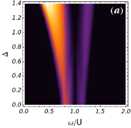
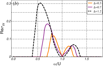
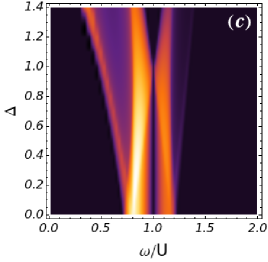
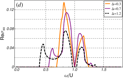
Figure 5: Analogous physical situation as in Fig. (4) but with non-zero amplitude of uniform magnetic field (half magnetic-flux per unit cell).

III.2 Connection to experiment

Recently, A. Tokuno and T. Giamarchi Tokuno and Giamarchi (2011) have proposed a spectroscopic technique for cold atoms which is able to extract current-current correlation function $\Pi_{xx}(\omega)$ (Eq. (14)). This function is proportional to OC $\sigma_{xx}^{\mathbf{A}_{0}}(\omega)$ (see Eq. (13)), which offers a possibility to probe the transport phenomena in the thermodynamic limit. Using the energy absorption rate techniques (EAR) such a goal could be achieved by phase modulation of optical lattice.

Namely, a vector potential $\mathbf{A}_{0}$ could be created in different experimental configurations Aidelsburger et al. (2011); Aidelsburger et al. (2013a); Struck et al. (2011). In our work we investigate the Landau gauge $\mathbf{A}_{0}=B(0,x,0)$ which generates a uniform magnetic field. Such a uniform field has been generated recently in Aidelsburger et al. (2013a) but using another type of effective vector potential. On the other hand, a small perturbing vector potential $\mathbf{A}^{\prime}$ could be generated by phase modulation of optical lattice Tokuno and Giamarchi (2011). If we consider a 2D system with $x$ and $y$ axes, we can generate a synthetic electric field $E\hat{x}$ by modulating the phase in the $x$ direction. This situation could be mathematically inferred from the exchange of a stationary optical lattice potential $V_{\textrm{op}}(\mathbf{r})=\cos^{2}\left(k_{x}x\right)+\cos^{2}\left(k_{y}y\right)$ to a time dependent one $V_{\textrm{op}}(\mathbf{r},t)$ where $x\rightarrow x-f_{x}\cos\left(\omega t\right)$ ($f_{x}$ is the strength of modulation which should be much smaller than a lattice constant). Such a phase modulation (PM) could be realized by e.g. a recently proposed phase controller Sadgrove and Nakagawa (2011). This leads us to the expression where EAR is given by Tokuno and Giamarchi (2011)

$$R_{\textrm{PM}}(\omega)=-\frac{1}{2}\omega^{3}f_{x}^{2}\Im\tilde{\Pi}_{xx}(\omega)\;,$$ (29)

in which $\tilde{\Pi}_{xx}(\omega)$ corresponds to $\Pi_{xx}(\omega)$ from Eq. (14) but with exchange $e^{*}\rightarrow M$ ($M$ is effective mass of an atom) Tokuno and Giamarchi (2011). To ensure a linear response regime and no dynamical phase transition the condition $\omega f_{x}\ll 1$ should be satisfied Eckardt et al. (2005); Drese and Holthaus (1997). The calculation of $R_{\textrm{PM}}(\omega)$ is made following a procedure similar to that used in the OC case where the current-current correlation function $\Pi_{xx}(i\omega)$ was also considered (see Eq. (13)). Fig. (6) presents a plot of $R_{\textrm{PM}}/\tilde{\sigma}_{Q}f_{x}^{2}$ for the uniform magnetic field of a strength $f=0,\;1/2,\;1/4$ on the square lattice in the zero temperature limit (here $\tilde{\sigma}_{q}=M^{2}/h$ is an effective quantum resistance). We see that the factor $\omega^{3}$ changes significantly the weight of the response in comparison to the OC given in Fig. 1 and therefore the higher frequency peaks give a grater contribution to the absorbed energy rate. The similarity of the shape of current-current correlation function and tight-binding dispersion in a strong magnetic field could be an indirect method of checking the Hofstadter spectrum in the BHM system Powell et al. (2010); Hofstadter (1976) where the center of the band is located around $\omega=U$.

The plots of EAR for the OC with staggered potential will be analogous to the case of a uniform field (discussed above) so we omit its graphical representation.

Summarizing, the EAR technique is directly related to OC and may act as a probe of transport phenomena using ultra-cold quantum gases. It is worth pointing out that the phase modulation is independent of the strength of the lattice potential in contrast to the amplitude modulation method Tokuno and Giamarchi (2011).

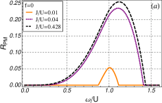
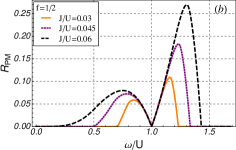
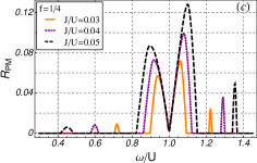
Figure 6: Imaginary part of current-current correlation function in two-dimensional square lattice in Mott phase (first lobe) is sketched in $\tilde{\sigma}_{Q}f_{x}^{2}$ units. From left - $f=0$ (a), $f=\frac{1}{2}$ (b), $f=\frac{1}{4}$ (c). Figures are plotted at zero temperature for different values of $J/U$.

III.3 Critical conductivity at the MI-SF phase boundary

III.3.1 The uniform field

Up to now the problem of critical conductivity in 2D on the Mott insulator - superfluid phase boundary in strong magnetic field has been rarely studied because of its complexity. The amplitude of the hopping term with a complex factor (see Eq. (5)) is the reason why in Ref. Cha and Girvin (1994) instead of BHM at integer filling, the frustrated XY model was investigated using the MC numerical method. Another approach to the problem of critical conductivity in magnetic field has been proposed in Ref. Nishiyama (2001), but the magnetic field considered there was weaker (i.e. $f=1/20$) than that the field we studied and their calculations were performed in the hard-core limit (the author used exact diagonalization method to overcome the difficulties related to the complex hopping term). Within the approach presented in this paper we can perform analytical analysis and study critical behavior of conductivity in a much wider range of magnetic fields. Namely, we show that for commensurate value of $f$, critical conductivity depends only on the number of minima located in the first reduced magnetic Brillouin zone.

To describe the critical conductivity at the tip of the Mott lobe Sinha and Sengupta (2011) we compute the OC (Eq. (III.1.1)) close to the phase boundary. To do that, in the following calculations, we consider only the real part of $\sigma_{xx}^{\mathbf{A}_{0}}(\omega)$ that gives a finite frequency contribution, namely the part of OC which consists of the current-current correlation function

$$\textrm{Re}\tilde{\sigma}_{xx}^{\mathbf{A}_{0}}(i\omega)=-\textrm{Re}\left\{\frac{2\pi}{R_{q}}\frac{1}{\hbar\beta N}\frac{1}{\hbar\omega}\frac{1}{\hbar}\sum_{\mathbf{k}n}\sum_{\alpha=0}^{q-1}\times\right.$$ (30)

$$\left.\left[\partial_{k_{x}}\epsilon_{q}^{\alpha}(\mathbf{k};p)\right]^{2}\mathcal{G}_{\alpha\alpha}^{d}(\mathbf{k},i\omega_{n})\mathcal{G}_{\alpha\alpha}^{d}(\mathbf{k},i\omega_{n}+i\omega)\right\}\;,$$

where $R_{q}=h/\left(e^{*}\right)^{2}=\sigma_{Q}^{-1}$ is quantum resistance (for Cooper pair $e^{*}=2e$ and $R_{q}\approx 6,45\;k\Omega$) and we restore the constant $\hbar$ to introduce it in quantum resistance $R_{q}$. Eq. (30) also contains the singular part of OC, but since we are interested in the Mott phase, we neglect this contribution further on.

Now, using the effective action from Eq. (10), and applying the Ginzburg-Landau (GL) like method for calculation of critical conductivity Kampf and Zimanyi (1993), we evaluate Eq. (30) in order to obtain its dependence on $f=p/q$ parameter. Following this procedure, we expand the action Eq. (10) to the second order in frequency using the expression

$$1-\epsilon_{q}^{\alpha}(\mathbf{k};p)G_{0}(i\omega_{n})=a_{\mathbf{k}}-b_{\mathbf{k}}i\hbar\omega_{n}-c_{\mathbf{k}}\left(i\hbar\omega_{n}\right)^{2}\;,$$ (31)

with

$$a_{\mathbf{k}}=1-\epsilon_{q}^{\alpha}(\mathbf{k};p)G_{0}(i\omega_{n}=0),$$ (32)

$$b_{\mathbf{k}}=\epsilon_{q}^{\alpha}(\mathbf{k};p)\partial_{r}G_{0}(r)|_{r=0}\,,\quad c_{\mathbf{k}}=\frac{1}{2}\epsilon_{q}^{\alpha}(\mathbf{k};p)\partial_{r}^{2}G_{0}(r)|_{r=0}\;.$$

Next, in calculating the critical conductivity within the GL action, we should assume the proper ground state behavior. From all set of $q-$band energy dispersion, we choose the lowest one which correctly reproduces the phase transition. This band contains $q$ GL modes in the first magnetic Brillouin zone (MBZ) Sinha and Sengupta (2011), which allows description of the critical behavior of the BHM close to the phase boundary. Going further we perform the summation over Matsubara frequencies and take the limit $T\rightarrow 0$, which reduces Eq. (30) to

$$\textrm{Re}\tilde{\sigma}_{xx}^{\mathbf{A}_{0}}(\omega)_{\textrm{}}=\frac{\pi^{2}}{R_{q}}\frac{1}{N}\sum_{\mathbf{k}\mathbf{Q}}\frac{\left(\mathbf{k}-\mathbf{Q}\right)^{2}}{m_{eff}^{2}\Delta_{\mathbf{k}}^{2}}\frac{2J^{2}}{(\epsilon_{q}^{\alpha}(\mathbf{k};p))^{2}}\delta\left(\omega^{2}-\frac{\Delta_{\mathbf{k}}^{2}}{c_{\mathbf{k}}^{2}}\right),$$ (33)

where $\Delta_{\mathbf{k}}=\sqrt{b_{\mathbf{k}}^{2}+4a_{\mathbf{k}}c_{\mathbf{k}}}$, $m_{eff}=1/\left.\partial_{k_{x}}^{2}\epsilon_{q}^{\alpha}(\mathbf{k};p)\right|{}_{\mathbf{k}=\mathbf{Q}}$ and $\mathbf{Q}$ are locations of the minima in MBZ. Close to the phase boundary only the momenta around $\mathbf{Q}$ bring a contribution to conductivity, therefore if the minimum of $\epsilon_{q}^{\alpha}(\mathbf{k};p)$ is located at $\mathbf{k}=\mathbf{Q}$ we can simply expand $a_{\mathbf{k}}$ from Eq. (32) to the second order

$$a_{\mathbf{k}}\approx\frac{\left(\mathbf{k}-\mathbf{Q}\right)^{2}}{2zJm_{eff}}$$ (34)

where $z=\epsilon_{q}^{\alpha}(\mathbf{Q};p)$ for chosen $p,\;q$. In further calculations we assume that $\partial_{k_{x}}^{2}\epsilon_{q}^{\alpha}(\mathbf{k};p)=\partial_{k_{y}}^{2}\epsilon_{q}^{\alpha}(\mathbf{k};p)$. Finally, for the point in the phase diagram which is close to the tip of the lobe, we get

$$\textrm{Re}\tilde{\sigma}_{xx}^{\mathbf{A}_{0}}(\omega)_{\textrm{}}=\frac{\pi}{8R_{q}}\sum_{\mathbf{Q}}\frac{\omega^{2}-\left(\frac{b_{\mathbf{Q}}}{c_{\mathbf{\mathbf{Q}}}}\right)^{2}}{\omega^{2}}\Theta\left(\omega^{2}-\frac{b_{\mathbf{Q}}^{2}}{c_{\mathbf{\mathbf{Q}}}^{2}}\right)\;,$$ (35)

where $\Theta(x)$ is a step function being non-zero for $x\geqslant 0$. The above expression describes the behavior of optical conductivity close to the phase transition. It has non-vanishing amplitude when the applied frequency is equal to $b_{\mathbf{Q}}/c_{\mathbf{\mathbf{Q}}}$ or is higher than this value. Denoting $\sigma^{*}=\pi\sigma_{Q}/8=\pi/8R_{q}$ and considering the tip of the lobe, where $b_{\mathbf{Q}}=0$ is the critical conductivity, $\textrm{Re}\tilde{\sigma}_{xx}^{\mathbf{A}_{0}}(\omega)\equiv\sigma_{c,f}$ takes the simple form

$$\sigma_{c,f}=q\sigma^{*}\;.$$ (36)

It is important to notice that theory presented here is valid for the second order phase transition, e.g. this condition is satisfied for the cases $f=1/2,\;1/3$ Cha and Girvin (1994).

f	normalized critical conductivity $\sigma_{c,f}\textrm{/}\sigma_{c,0}$
	MKF (here)	XY model	MC	JJA experiment
1/2	2	2	1,82	$\approx 2$
1/3	3		2,91	$\approx 3$
1/q	q			$\approx q$

Table 1: Comparison of critical conductivity for different magnetic field configuration calculations Granato and Kosterlitz (1990); Grason and Bruinsma (2006); Cha et al. (1991); Cha and Girvin (1994) and experimental measurements van der Zant et al. (1992); van der Zant H. S. et al. (1996).

To discuss the result from Eq. (36) we firstly recall that for the simplest case $q=1$ where there is no magnetic field, the result for $q=1$ confirms the results presented in Refs. Cha et al. (1991); Kampf and Zimanyi (1993); van Otterlo et al. (1993). With $p/q=1/2$ we have $\sigma_{c,1/2}=2\sigma^{*}$. This result agrees with the analytical solution given in Refs. Grason and Bruinsma (2006); Granato and Kosterlitz (1990), where the XY model was used. Also in the MC study for $f=1/2$ Cha and Girvin (1994) a value of critical conductivity is $1,82$ times higher than for $f=0$ Cha et al. (1991). Results of an experiment conducted in Josephson junction arrays van der Zant et al. (1992); van der Zant H. S. et al. (1996) also show a similar behavior. If we consider $f=1/3$, it qualitatively agrees with the Monte Carlo result in Ref. Cha and Girvin (1994), where Cha and Grivin obtained $2,91$ higher value of critical conductivity than in the absence of a magnetic field. The authors of the experimental work, in Refs. van der Zant et al. (1992); van der Zant H. S. et al. (1996) also discuss such a scenario. It is worth adding that the authors of Ref. Granato and Kosterlitz (1990) have speculated about a similar result for $\sigma_{c,1/3}$ i.e. $\sigma_{c,1/3}=3\sigma_{c,0}$. Namely, they have suggested that at least for low order rationals of $p/q$ critical conductivity could satisfy Eq. (36) but they have carried out explicit calculation only for $f=1/2$. In contrast, we showed this behavior by analytical methods for arbitrary $f$ within a clear mathematical framework. The above considerations are summarized in Table 1. It is worth mentioning that in three dimensions a trivial solution $\sigma_{c,f}=0$ is obtained, known before only for the case of $f=0$ (e.g, see Kampf and Zimanyi (1993)).

For Josephson junction arrays (JJA) it seems that the critical conductivity is proportional to $q/p$ van der Zant H. S. et al. (1996) but this linear behavior is inferred from a small number of experimental points with a large error margin. Therefore, such a dependence is still an open question. Moreover, in (JJA) we should take into account that arrays are not perfect and their parameters differ through the network. Also, the measurements are performed at finite temperatures. For example, if we consider a disorder we should expect that this effect suppresses the value of critical conductivity Sø rensen et al. (1992); Cha and Girvin (1994). It is worth mentioning here that also long range interactions which we neglected could have a significant impact Sø rensen et al. (1992). Besides, it seems that $\sigma_{c,f}$ should depend on $p$. Hence our results (36) within the approximations used in this paper should be at least appropriate for $p\approx 1$.

III.3.2 The uniform field (f=1/2) with uniaxially staggered potential

To show the importance of translation symmetry breaking by the uniaxially staggered potential in a special case $f=1/2$ Delplace and Montambaux (2010), we analyze the critical behavior of conductivity at the phase boundary.

Following the same procedure for the critical conductivity which led us to Eq. (36) we simply observe that for $\Delta=0$ (for definition of parameter $\Delta$ see Sec. III.1.2) we get $\sigma_{c,f}=2\sigma^{*}$. But for $\Delta>0$, the situation is changed significantly. Analysis of the spectrum of quasi-particles in the Mott phase reveals that one of the two minima disappears in the first magnetic Brillouin zone for the non-zero value of $\Delta$ (see Fig. 7). Therefore, there exists only the one lowest energy Ginzburg-Landau mode which effectively recovers the critical conductivity as when there is no magnetic field. Hence, such an abrupt change in the critical value of $\sigma_{c,f}$ from $2\sigma^{*}$ to $\sigma^{*}$when the staggered potential is turned on, could be an interesting effects on its own right. In addition, no variation in the critical conductivity for $f=0$ was observed.

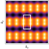
Figure 7: Above we sketch density plot of the lowest band energy in the Mott phase (white rectangle describe first magnetic Brillouin zone (MBZ)). The range from darker to brighter color is assigned to the lowest and highest value of energy spectrum respectively. Pictures have $\Delta=0$ and $\Delta=0.7$ (from left). We see explicitly disappearance one of the two minima (black color) on the center of the MBZ.

The best options to study the presented effects in experiments that could be made nowadays is the use of optical lattices with ultra-cold atoms whose high controllability provides a better road to connect experiment and theory. The continuous progress in ultra-cold quantum gases in the near future also will allow getting into the temperature regime where high precision measurement of critical conductivity will be possible. This can verify the above results and allow omission of additional effects which occur in standard solid state devices like Josephson junction arrays. The possibility of such measurements has been very recently discussed in Ref. Chen et al. (2013).

The analysis made in Sec. III.3 permits a better understanding of the superconductor-insulator phase transition mechanism. To illustrate this, we shortly explain below the fact that the critical conductivity should be affected by the applied magnetic field. Namely, we know that the scenario of critical resistance (i.e. $1/\sigma_{c,f}$) is assigned to the vortex and boson flowing through the system at the critical transition point Cha et al. (1991). Such a description is possible from the duality transformation Fisher et al. (1990); Fisher (1990) (e.g. for superconductor-insulator transition induced in a fermionic system these bosons are Cooper pairs with short coherence length Cha et al. (1991)). Therefore, application of a magnetic field at least affects the behavior of vortices, which changes the critical resistance. In our calculations the magnetic field is effectively incorporated into the theory through the tight binding dispersion relation $\epsilon_{q}^{\alpha}(\mathbf{k};p)$ which gives $q-$bands spectrum with $q$ minima in the lowest energy level, what finally changes $\sigma_{c,f}$. If we additionally consider the staggered potential, an analogous prediction could be made.

IV Summary

The analysis of conductivity in BHM in a strong magnetic field is challenging problem due to complex hopping term. In particular, up to now its optical dependence was out of reach in Monte Carlo study. Therefore our theory expands the area in which numerical methods are used.

Namely, we have proposed the magnetic Kubo formula which is valid for an arbitrary flux pattern where commensurability effects of a magnetic field are included. Within this framework, we have calculated the optical conductivity in the Mott phase of the Bose Hubbard model and considered its critical value. To check our results we have proposed to compare them with presently available experiment in ultra-cold quantum gases in which current-current correlation function in a uniform magnetic field could be probed. Such a connection of experiments and theory could open a new avenue to study transport phenomena in highly controllable magnetic field where geometry of the lattice can be easily manipulated. Moreover, for the case of critical conductivity we have shown its dependence on the topology of the single-particle spectrum and obtained solution which are in good agreement with presently available numerical and experimental data.

The method presented here can be extended over many-body systems in which the strong magnetic field plays a significant role.

V Appendix

Here we present the quasi-particle energy spectrum and densities of states for conductivity (DOSc) in 2D described in Sec. III.1. We use $\mathcal{K}$ and $\mathcal{E}$ to denote the first and second complete elliptic integral, respectively.

V.1 Uniform magnetic field for a two-dimensional square lattice

V.1.1 f=0

The dispersion relation for the square lattice is

$$\epsilon_{1}^{\alpha}(\mathbf{k};0)=-2J\left(\cos k_{x}+\cos k_{y}\right),$$ (37)

where the DOSc (Eq. (27) is given by Belkhir and Randeria (1994)

$$\rho_{1}^{0}(E;0)=\frac{4\Theta\left(4-|E|\right)}{\pi^{2}}\left[\mathcal{E}\left(\sqrt{1-\left(\frac{E}{4}\right)^{2}}\right)-\left(\frac{E}{4}\right)^{2}\mathcal{K}\left(\sqrt{1-\left(\frac{E}{4}\right)^{2}}\right)\right].$$ (38)

V.1.2 f=1/2

The dispersion relation for $f=1/2$ is built from two sub-bands Hasegawa et al. (1989) $\pm 2\sqrt{\cos^{2}k_{x}+\cos k_{y}^{2}}$ and consequently the DOSc is

$$\rho_{2}^{\alpha}(E;1)=\frac{4\Theta_{\alpha}}{\pi^{2}|E|}\left[\mathcal{E}\left(\sqrt{1-\left(\frac{E^{2}-4}{4}\right)^{2}}\right)-\left(\frac{E^{2}-4}{4}\right)^{2}\mathcal{K}\left(\sqrt{1-\left(\frac{E^{2}-4}{4}\right)^{2}}\right)\right]\;,$$ (39)

where $\Theta_{\alpha}$ is non-zero step function within each q-band.

V.1.3 f=1/4

The form of dispersion relation $f=1/4$ is expressed by four sub-bands Hasegawa et al. (1989) $\pm\sqrt{4-\sqrt{12+2\cos\left(4k_{x}\right)+2\cos\left(4k_{y}\right)}}$ and $\pm\sqrt{4+\sqrt{12+2\cos\left(4k_{x}\right)+2\cos\left(4k_{y}\right)}}$, then we get

$$\rho_{4}^{\alpha}(E;1)=\frac{4\Theta_{\alpha}}{\pi^{2}\left|E^{2}-4\right||E|}\left[\mathcal{E}\left(\sqrt{1-\left(\frac{4-8E^{2}+E^{4}}{4}\right)^{2}}\right)-\left(\frac{4-8E^{2}+E^{4}}{4}\right)^{2}\mathcal{K}\left(\sqrt{1-\left(\frac{4-8E^{2}+E^{4}}{4}\right)^{2}}\right)\right]\;.$$ (40)

V.2 Uniform magnetic field for a two-dimensional square lattice with uniaxially staggered potential

V.2.1 f=0

The form of tight binding dispersion has two sub-bands Delplace and Montambaux (2010) $-2J\cos k_{y}\pm 2J\sqrt{\cos^{2}k_{x}+\Delta^{2}}$ and the appropriate DOSc is given by

- for $xx$ component of optical conductivity $\sigma_{xx}^{\mathbf{A}_{0}}(\omega)$:

$$\rho_{2}^{\alpha}(E;1)=\frac{2\Theta_{\alpha}}{\pi^{2}}\int_{0}^{1}dx\,\frac{x^{2}}{x^{2}+\Delta^{2}}\frac{\sqrt{1-x^{2}}}{\sqrt{1-\left(\frac{E}{2}\pm\sqrt{x^{2}+\Delta^{2}}\right)^{2}}}\;,$$ (41)

- for $yy$ component of optical conductivity $\sigma_{yy}^{\mathbf{A}_{0}}(\omega)$:

$$\rho_{2}^{\alpha}(E;1)=\frac{2\Theta_{\alpha}}{\pi^{2}}\int_{0}^{1}dx\,\frac{\sqrt{1-\left(\frac{E}{2}\pm\sqrt{x^{2}+\Delta^{2}}\right)^{2}}}{\sqrt{1-x^{2}}}\;.$$ (42)

V.2.2 f=1/2

The form of tight binding dispersion has two sub-bands Delplace and Montambaux (2010) $\pm 2\sqrt{\cos^{2}k_{x}+\left(\cos k_{y}-\Delta\right)^{2}}$ and the appropriate DOSc is given by

- for $xx$ component of optical conductivity $\sigma_{xx}^{\mathbf{A}_{0}}(\omega)$:

$$\rho_{2}^{\alpha}(E;1)=\frac{4\Theta_{\alpha}}{\pi^{2}|E|}\int_{-1-\Delta}^{1-\Delta}dx\,\frac{\sqrt{\left(\frac{E}{2}\right)^{2}-x^{2}}\sqrt{1-\left(\frac{E}{2}\right)^{2}+x^{2}}}{\sqrt{1-\left(x+\Delta\right)^{2}}}\;,$$ (43)

- for $yy$ component of optical conductivity $\sigma_{yy}^{\mathbf{A}_{0}}(\omega)$:

$$\rho_{2}^{\alpha}(E;1)=\frac{4\Theta_{\alpha}}{\pi^{2}|E|}\int_{-1-\Delta}^{1-\Delta}dx\,\frac{x^{2}}{\sqrt{\left(\frac{E}{2}\right)^{2}-x^{2}}}\frac{\sqrt{1-\left(x+\Delta\right)^{2}}}{\sqrt{1-\left(\frac{E}{2}\right)^{2}+x^{2}}}\;.$$ (44)

References

- Micnas et al. (1990) R. Micnas, J. Ranninger, and S. Robaszkiewicz, Rev. Mod. Phys. 62, 113 (1990).
- Cha and Girvin (1994) M. C. Cha and S. M. Girvin, Phys. Rev. B 49, 9794 (1994).
- van Otterlo et al. (1993) A. van Otterlo, K. H. Wagenblast, R. Fazio, and G. Schön, Phys. Rev. B 48, 3316 (1993).
- Greiner et al. (2002) M. Greiner, O. Mandel, T. Esslinger, T. Hänsch, and I. Bloch, Nature 415, 39 (2002).
- Stöferle et al. (2004) T. Stöferle, H. Moritz, C. Schori, M. Köhl, and T. Esslinger, Phys. Rev. Lett. 92, 130403 (2004).
- Jaksch and Zoller (2005) D. Jaksch and P. Zoller, Ann. Phys. (N. Y). 315, 52 (2005).
- Saha et al. (2010) K. Saha, K. Sengupta, and K. Ray, Phys. Rev. B 82, 205126 (2010).
- Powell et al. (2010) S. Powell, R. Barnett, R. Sensarma, and S. Das Sarma, Phys. Rev. Lett. 104, 255303 (2010).
- Zaleski and Polak (2011) T. A. Zaleski and T. P. Polak, Phys. Rev. A 83, 023607 (2011).
- Powell et al. (2011) S. Powell, R. Barnett, R. Sensarma, and S. Das Sarma, Phys. Rev. A 83, 013612 (2011).
- Sinha and Sengupta (2011) S. Sinha and K. Sengupta, EPL (Europhysics Lett. 93, 30005 (2011).
- Nakano et al. (2012) Y. Nakano, K. Kasamatsu, and T. Matsui, Phys. Rev. A 85, 023622 (2012).
- Polak and Zaleski (2013) T. P. Polak and T. A. Zaleski, Phys. Rev. A 87, 033614 (2013).
- Struck et al. (2013) J. Struck, M. Weinberg, C. Ölschläger, P. Windpassinger, J. Simonet, K. Sengstock, R. Höppner, P. Hauke, A. Eckardt, M. Lewenstein, et al., Nat. Phys. 9, 738 (2013).
- Šmakov and Sø rensen (2005) J. Šmakov and E. Sø rensen, Phys. Rev. Lett. 95, 180603 (2005).
- Bhaseen et al. (2007) M. J. Bhaseen, A. G. Green, and S. L. Sondhi, Phys. Rev. Lett. 98, 166801 (2007).
- Bhaseen et al. (2009) M. J. Bhaseen, A. G. Green, and S. L. Sondhi, Phys. Rev. B 79, 094502 (2009).
- Lindner and Auerbach (2010) N. H. Lindner and A. Auerbach, Phys. Rev. B 81, 054512 (2010).
- Tokuno and Giamarchi (2011) A. Tokuno and T. Giamarchi, Phys. Rev. Lett. 106, 205301 (2011).
- Chen et al. (2013) K. Chen, L. Liu, Y. Deng, L. Pollet, and N. Prokof’ev, pp. 1–7 (2013), eprint arXiv:1309.5635v1.
- Kessler and Marquardt (2013) S. Kessler and F. Marquardt, pp. 1–8 (2013), eprint arXiv:1309.3890v1.
- van der Zant et al. (1992) H. S. J. van der Zant, L. J. Geerligs, and J. E. Mooij, EPL 19, 541 (1992).
- van der Zant H. S. et al. (1996) van der Zant H. S., W. J. Elion, L. J. Geerligs, and J. E. Mooij, Phys. Rev. B. Condens. Matter 54, 10081 (1996).
- Lin et al. (2009) Y.-J. Lin, R. L. Compton, K. Jiménez-García, J. V. Porto, and I. B. Spielman, Nature 462, 628 (2009).
- Aidelsburger et al. (2011) M. Aidelsburger, M. Atala, S. Nascimbène, S. Trotzky, Y.-A. Chen, and I. Bloch, Phys. Rev. Lett. 107, 255301 (2011).
- Aidelsburger et al. (2013a) M. Aidelsburger, M. Atala, M. Lohse, J. T. Barreiro, B. Paredes, and I. Bloch, Phys. Rev. Lett. 111, 185301 (2013a).
- Miyake et al. (2013) H. Miyake, G. A. Siviloglou, C. J. Kennedy, W. C. Burton, and W. Ketterle, Phys. Rev. Lett. 111, 185302 (2013).
- Struck et al. (2011) J. Struck, C. Ölschläger, R. Le Targat, P. Soltan-Panahi, A. Eckardt, M. Lewenstein, P. Windpassinger, and K. Sengstock, Science 333, 996 (2011).
- Sø rensen et al. (2005) A. S. Sø rensen, E. Demler, and M. D. Lukin, Phys. Rev. Lett. 94, 086803 (2005).
- Jaksch and Zoller (2003) D. Jaksch and P. Zoller, New J. Phys. 5, 56 (2003).
- Nayak et al. (2008) C. Nayak, A. Stern, M. Freedman, and S. Das Sarma, Rev. Mod. Phys. 80, 1083 (2008).
- Hasan and Kane (2010) M. Z. Hasan and C. L. Kane, Rev. Mod. Phys. 82, 3045 (2010).
- Nishiyama (2001) Y. Nishiyama, Physica C Supercond. 353, 147 (2001).
- Wagenblast et al. (1997) K.-H. Wagenblast, A. van Otterlo, G. Schön, and G. T. Zimányi, Phys. Rev. Lett. 78, 1779 (1997).
- Kim and Stroud (2008) K. Kim and D. Stroud, Phys. Rev. B 78, 174517 (2008).
- Granato and Kosterlitz (1990) E. Granato and J. M. Kosterlitz, Phys. Rev. Lett. 65, 1267 (1990).
- Aidelsburger et al. (2013b) M. Aidelsburger, M. Atala, S. Nascimbène, S. Trotzky, Y.-A. Chen, and I. Bloch, Appl. Phys. B 113, 1 (2013b).
- Delplace and Montambaux (2010) P. Delplace and G. Montambaux, Phys. Rev. B 82, 035438 (2010).
- Fisher et al. (1990) M. P. A. Fisher, G. Grinstein, and S. M. Girvin, Phys. Rev. Lett. 64, 587 (1990).
- Grason and Bruinsma (2006) G. M. Grason and R. F. Bruinsma, Phys. Rev. Lett. 97, 027802 (2006).
- Sengupta and Dupuis (2005) K. Sengupta and N. Dupuis, Phys. Rev. A 71, 033629 (2005).
- Hasegawa et al. (1989) Y. Hasegawa, P. Lederer, T. M. Rice, and P. B. Wiegmann, Phys. Rev. Lett. 63, 907 (1989).
- Hofstadter (1976) D. R. Hofstadter, Phys. Rev. B 14, 2239 (1976).
- Kampf and Zimanyi (1993) A. P. Kampf and G. T. Zimanyi, Phys. Rev. B 47, 279 (1993).
- Wu and Phillips (2006) J. Wu and P. Phillips, Phys. Rev. B 73, 214507 (2006).
- Cha et al. (1991) M. C. Cha, M. P. A. Fisher, S. M. Girvin, M. Wallin, and A. P. Young, Phys. Rev. B 44, 6883 (1991).
- Wagenblast et al. (1996) K. H. Wagenblast, R. Fazio, A. van Otterlo, G. Schön, Z. Dario, and G. T. Zimanyi, Phys. B Condens. 222, 336 (1996).
- Dalidovich and Phillips (2001) D. Dalidovich and P. Phillips, Phys. Rev. B 64, 184511 (2001).
- Dalidovich and Phillips (2002) D. Dalidovich and P. Phillips, Phys. Rev. B 66, 073308 (2002).
- Sadgrove and Nakagawa (2011) M. Sadgrove and K. Nakagawa, Rev. Sci. Instrum. 82, 113104 (2011).
- Eckardt et al. (2005) A. Eckardt, C. Weiss, and M. Holthaus, Phys. Rev. Lett. 95, 260404 (2005).
- Drese and Holthaus (1997) K. Drese and M. Holthaus, Chem. Phys. 217, 201 (1997).
- Sø rensen et al. (1992) E. S. Sø rensen, M. Wallin, S. M. Girvin, and A. P. Young, Phys. Rev. Lett. 69, 828 (1992).
- Fisher (1990) M. P. A. Fisher, Phys. Rev. Lett. 65, 923 (1990).
- Belkhir and Randeria (1994) L. Belkhir and M. Randeria, Phys. Rev. B 49, 6829 (1994).