Uni-directional optical pulses and temporal propagation:
with consideration of spatial and temporal dispersion

Abstract

I derive a temporally propagated uni-directional optical pulse equation valid in the few cycle limit. Temporal propagation is advantageous because it naturally preserves causality, unlike the competing spatially propagated models. The exact coupled bi-directional equations that this approach generates can be efficiently approximated down to a uni-directional form in cases where an optical pulse changes little over one optical cycle. They also permit a direct term-to-term comparison of the exact bi-directional theory with its corresponding approximate uni-directional theory. Notably, temporal propagation handles dispersion in a different way, and this difference serves to highlight existing approximations inherent in spatially propagated treatments of dispersion. Accordingly, I emphasise the need for future work in clarifying the limitations of the dispersion conversion required by these types of approaches; since the only alternative in the few cycle limit may be to resort to the much more computationally intensive full Maxwell equation solvers.

I Introduction

The importance of having simple and robust methods for the propagation of optical pulses has attracted increasing attention in recent years. This is due to the multitude of applications Brabec and Krausz (2000) in which ever shorter pulses are used to act like a strobe-lamp that takes snapshots of ultrafast processes Corkum (1993); Schafer et al. (1993), or sub-wavelength electric field profiles are created Fuji et al. (2005); Radnor et al. (2008); Solanpää et al. (2014) to achieve detailed control over atomic or molecular responses. Alternatively, strong nonlinearity can be used to construct pulses that are both wide-band and temporally extended, such as (white light) supercontinnua Alfano and Shapiro (1970a, b); Dudley et al. (2006). Such nonlinearities can even be used to generate sub-structure that is instead temporally confined, as in optical rogue waves Solli et al. (2007); or even the temporally and spatially localized filamentation processes Braun et al. (1995); Chin et al. (1999); Milchberg et al. (2014).

This progress towards achieving ever shorter pulse durations, with their associated larger spectral bandwidths, and higher pulse intensities, has been pushing traditional pulse propagation models to their limits, or breaking them. If we want to avoid the computational expense of always resorting to high resolution Maxwell’s equations solvers coupled to detailed material response models, we need to be confident that our simpler, less demanding approaches still work. In particular we need to have a clear idea of the physics that may have been removed, and what the side-effects of those approximations are. In this paper I use a directional approach, whose relatively simple and straightforward derivation allows easy comparison of both the approximate and the exact propagation equations, whilst still resulting in the analytical and numerical convenience of a first-order wave equation.

However, unlike perhaps the most common approach in nonlinear optics, I consider propagation in time rather than along some chosen spatial axis Kinsler (2010, 2012a). The most significant distinctions between temporal and spatial propagation approaches are summarized on figs. 1 and 2 respectively. Notice that the initial conditions (starting states) are completely different, and that only the temporal propagation model is going to provide causal solutions in a straightforward way. The temporally propagated evolution equations for the spatial wave profiles do not give us access to the frequency spectrum Kinsler (2014), but instead we have the wavevector spectrum, as well as a causally appropriate time evolution Kinsler (2011). This requires an alternate approach to the temporal response of the propagation medium, which highlights the existing and often somewhat poorly characterised approximations inherent in spatially propagated treatments of dispersion. Of course, full finite element and/or FDTD Yee (1966) pulse propagation can also be used, but here my aim is to simplify the time propagated approach in a directional approach in line with common spatially propagated methods.

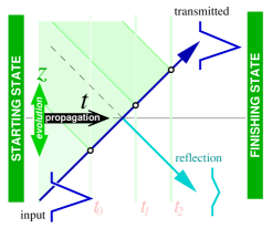
Figure 1: Temporal propagation of waves, where disturbances (or pulses) evolve either forward or backward in space. At any point in the propagation, we know the spatial behaviour of our wave field at all points in space, as indicated by the pale vertical lines. The pale shaded triangles indicate the past light cones (i.e. the causal past) of a wave element (black circles) at selected times along the path of the disturbance. In a temporally propagated numerical simulation which has a maximum wave speed, the causal past matches the computational past. A notional interface has been added to the diagram to show how a reflection would behave. Figure used with permission from Kinsler (2014).

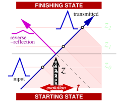
Figure 2: Spatial propagation of waves, where disturbances (or pulses) evolve either forward or backward in time. At any point in the propagation, we know the full time behaviour of our wave field – both history and future, as indicated by the pale horizontal lines.. The light shaded triangles indicates the computational past of a wave element at particular points (black circles) along the path of the disturbance. Note that unlike the temporally propagated case shown in fig. 1, the computational past of a spatially propagated system is not the same as the causal past. A notional interface has been added to the diagram to show how reflections behave – i.e. in an unexpected way Kinsler (2012b). This is because a reflection should have been put in the initial conditions, but was not due to an (assumed) lack of knowledge of that future behaviour. Figure used with permission from Kinsler (2014).

In section II I derive a customized second order wave equation from Maxwell’s equations, and reorganize it to define the material properties appropriately and set up the factorization stage. In section III, I use a factorization method Kinsler (2010) that allows us to construct an explicitly bi-directional model, and which is then approximated to the popular uni-directional limit in section IV. Section IV.4 remarks on commonly used modifications that can be applied to the equations given in sections III and IV, typically in order to clarify their properties, simplify them, or compare them to existing models. Having derived this main result – the propagation equations and their various specializations – I turn in section V to the consequences of temporal propagation and the perspective it provides on the handling of mixed spatial and temporal dispersive effects. This is then followed in section VI by a specific comparison between the ordinary spatially propagated nonlinear Schrödinger (NLS) equation – perhaps the most widely investigated equation in nonlinear optics – and its temporally propagated counterpart. Finally, in section VII, I present my conclusions.

II Second order wave equation

My starting point is the standard macroscopic Maxwell’s equations, where I aim for a solution based on a uniform and source free dielectric medium, but still intending to allow material properties that are as general as possible. A typical approach to this is to construct a second order wave equation for the electric field E, as results from the substitution of the $\nabla\times{\textbf{H}}=\partial_{t}{\textbf{D}}+{\textbf{J}}$ Maxwell’s equation into $\nabla\times{\textbf{E}}=-\partial_{t}{\textbf{B}}$ (see e.g. Agrawal (2007)). Here, however, I want to follow the displacement field D (not E) since it naturally occurs in conjuction with a time derivative – likewise, the other important field is B rather than H. Thus we rearrange the curl Maxwell’s equations to emphasize both their causal properties Kinsler (2011) and their time derivatives, as

$${\mu_{0}}\partial_{t}{\textbf{D}} ={\mu_{0}}\nabla\times{\textbf{H}}-{\mu_{0}}{\textbf{J}}\quad=\nabla\times{\textbf{B}}-{\mu_{0}}\nabla\times{\textbf{M}}-{\mu_{0}}{\textbf{J}},$$ (2.1)

$${\epsilon_{0}}\partial_{t}{\textbf{B}} =-{\epsilon_{0}}\nabla\times{\textbf{E}}-{\epsilon_{0}}{\textbf{K}}~{}~{}=-\nabla\times{\textbf{D}}+\nabla\times{\textbf{P}}-{\epsilon_{0}}{\textbf{K}}.$$ (2.2)

Note that for both of these equations, we will also (as usual) want to specify the material response, whether dielectric or magnetic, in terms of a dielectric polarization ${\textbf{P}}={\textbf{D}}-{\epsilon_{0}}{\textbf{E}}$ and a magnetization ${\textbf{M}}={\textbf{B}}-{\mu_{0}}{\textbf{H}}$. Either of these equations given above might be either in the spatial domain (with argument $\textbf{r}=(r_{x},r_{y},r_{z})$), or the wavevector domain (with argument $\textbf{k}=(k_{x},k_{y},k_{z})$).

Now we define the total magnetization M in terms of a component ${\textbf{M}}_{L}$ linearly dependent on B, and another component ${\textbf{M}}_{\textup{B}}$ containing the rest. As a result, the excess polarization ${\textbf{M}}_{\mu}\equiv{\textbf{M}}_{\textup{B}}$, which will typically include any nonlinearity, is also a function of B and not H. In traditional H-based spatially-propagated approaches, the temporal response (“dispersion”) can be incorporated naturally, here it cannot. We have that

$${\textbf{M}}(\textbf{r}) ={\textbf{M}}_{L}(\textbf{r})+{\textbf{M}}_{\textup{B}}(\textbf{r}) =\alpha_{\mu}(\textbf{r}){\textbf{B}}(\textbf{r})+{\textbf{M}}_{\textup{B}}(\textbf{r}),$$ (2.3)

which in the spatial frequency (wavevector k) domain is

$${\textbf{M}}(\textbf{k}) ={\textbf{M}}_{L}(\textbf{k})+{\textbf{M}}_{\textup{B}}(\textbf{k}) =\alpha_{\mu}(\textbf{k})\star{\textbf{B}}(\textbf{k})+{\textbf{M}}_{\textup{B}}(\textbf{k}),$$ (2.4)

since after a Fourier transform from r into k, the products become spatial convolutions (“$\star$”); which emphasises that anything wavevector dependent is necessarily a non-local concept. Note that this is the converse of the usual situation where a temporal response is described using time-domain convolutions, and these become products in the frequency domain.

Now we define the total polarization P in terms of a component ${\textbf{P}}_{L}$ linearly dependent on D, and another component ${\textbf{P}}_{\textup{D}}$ containing the rest. As a result, the excess polarization ${\textbf{P}}_{\epsilon}\equiv{\textbf{P}}_{\textup{D}}$, which will typically include any nonlinearity, is also a function of D. We have that

$${\textbf{P}}(\textbf{r}) ={\textbf{P}}_{L}(\textbf{r})+{\textbf{P}}_{\textup{D}}(\textbf{r}) =\alpha_{\epsilon}(\textbf{r}){\textbf{D}}(\textbf{r})+{\textbf{P}}_{\textup{D}}(\textbf{r}),$$ (2.5)

which in the spatial frequency (wavevector k) domain is

$${\textbf{P}}(\textbf{k}) =\alpha_{\epsilon}(\textbf{k})\star{\textbf{D}}(\textbf{k})+{\textbf{P}}_{\textup{D}}(\textbf{k}).$$ (2.6)

With these definitions for $\partial_{t}{\textbf{D}}$, $\partial_{t}{\textbf{B}}$, and for M and P set up, we can now proceed with the derivation of a second order wave equation for D –

$${\mu_{0}}\partial_{t}{\textbf{D}} =\nabla\times{\textbf{B}}-{\mu_{0}}\nabla\times{\textbf{M}}_{L}-{\mu_{0}}\nabla\times{\textbf{M}}_{\textup{B}}-{\mu_{0}}{\textbf{J}}$$ (2.7)

$$=\nabla\times{\textbf{B}}-\nabla\times\alpha_{\mu}{\textbf{B}}-{\mu_{0}}\nabla\times{\textbf{M}}_{\textup{B}}-{\mu_{0}}{\textbf{J}}$$ (2.8)

$$=\nabla\times{\textbf{B}}-\alpha_{\mu}\nabla\times{\textbf{B}}-\left(\nabla\alpha_{\mu}\right)\times{\textbf{B}}-{\mu_{0}}\nabla\times{\textbf{M}}_{\textup{B}}-{\mu_{0}}{\textbf{J}}$$ (2.9)

$$=\nabla\times\left[1-\alpha_{\mu}\right]{\textbf{B}}-{\mu_{0}}\nabla\times{\textbf{M}}_{\textup{B}}-{\mu_{0}}{\textbf{J}}.$$ (2.10)

Now take the time derivative of this equation, use the fact that $\alpha_{\mu}$ is independent of time, define ${a}_{\mu}=1-\alpha_{\mu}$ and ${a}_{\epsilon}=1-\alpha_{\epsilon}$; and then substitute for $\partial_{t}{\textbf{B}}$, so that

$${\epsilon_{0}}{\mu_{0}}\partial_{t}^{2}{\textbf{D}} ={\epsilon_{0}}\nabla\times{a}_{\mu}\partial_{t}{\textbf{B}}-{\epsilon_{0}}{\mu_{0}}\nabla\times\partial_{t}{\textbf{M}}_{\textup{B}}-{\epsilon_{0}}{\mu_{0}}\partial_{t}{\textbf{J}}$$ (2.11)

$$c^{-2}\partial_{t}^{2}{\textbf{D}} =-\nabla\times{a}_{\mu}\left[\nabla\times{\textbf{D}}-\nabla\times{\textbf{P}}+{\epsilon_{0}}{\textbf{K}}\right]$$

$$\qquad\qquad-c^{-2}\nabla\times\partial_{t}{\textbf{M}}_{\textup{B}}-c^{-2}\partial_{t}{\textbf{J}}$$ (2.12)

$$\partial_{t}^{2}{\textbf{D}} =-{c}^{2}\nabla\times{a}_{\mu}\left[\nabla\times{\textbf{D}}-\nabla\times\alpha_{\epsilon}{\textbf{D}}-\nabla\times{\textbf{P}}_{\textup{D}}+{\epsilon_{0}}{\textbf{K}}\right]$$

$$\qquad\qquad-\nabla\times\partial_{t}{\textbf{M}}_{\textup{B}}-\partial_{t}{\textbf{J}}$$ (2.13)

$$=-{c}^{2}\nabla\times{a}_{\mu}\left[\nabla\times\left(1-\alpha_{\epsilon}\right){\textbf{D}}-\nabla\times{\textbf{P}}_{\textup{D}}+{\epsilon_{0}}{\textbf{K}}\right]$$

$$\qquad\qquad-\nabla\times\partial_{t}{\textbf{M}}_{\textup{B}}-\partial_{t}{\textbf{J}}$$ (2.14)

$$=-{c}^{2}\nabla\times{a}_{\mu}\nabla\times{a}_{\epsilon}{\textbf{D}}+{c}^{2}\nabla\times{a}_{\mu}\nabla\times{\textbf{P}}_{\textup{D}}$$

$$\qquad\qquad-{c}^{2}\nabla\times{a}_{\mu}{\epsilon_{0}}{\textbf{K}}-\nabla\times\partial_{t}{\textbf{M}}_{\textup{B}}-\partial_{t}{\textbf{J}}$$ (2.15)

Remember that in this picture, all field properties are specified as functions of our chosen primary field D; notably, the magnetic field B which is usually the main argument for ${\textbf{M}}_{\textup{B}}$ must be determined from the calculated D using the relevant Maxwell’s equation (i.e. eqn. (2.2)).

II.1 Simple case: isotropic & homogeneous

Since trying to treat all the details of eqn. (2.15) correctly leads to excessively complicated expressions, I will first simplify it down into the case where (a) the material’s reference properties ${a}_{\mu}$, ${a}_{\epsilon}$ do not vary in space, and (b) the effective monopole current is zero (${\textbf{K}}=0$). Since (magnetic) monoples do not exist, and all non reference properties can still be encoded in ${\textbf{P}}_{\textup{D}}$, ${\textbf{M}}_{\textup{B}}$, or J, this simplification does not (of itself) impose any approximation. However, the first simplification means that our reference properties cannot incorporate any exact knowledge about the spatial structure of the propagation medium. This restriction on obtaining the best possible match between the reference behaviour and the exact behaviour of the propagation medium will typically affect later approximations, where we assume deviations from the reference behaviour are small. One additional advantage of selecting constant reference parameters $\alpha_{\mu}$ and $\alpha_{\epsilon}$ is that we can easily replace them with matrices to allow for e.g. birefringence and cross-polarization couplings.

The simplified second order wave equation for changes in the displacement field ${\textbf{D}}(\textbf{r})$ as it propagates forward in time is

$$\partial_{t}^{2}{\textbf{D}} =-{c}^{2}{a}_{\mu}{a}_{\epsilon}\nabla\times\nabla\times{\textbf{D}}\quad+{c}^{2}{a}_{\mu}\nabla\times\nabla\times{\textbf{P}}_{\textup{D}}$$

$$\qquad\qquad-\nabla\times\partial_{t}{\textbf{M}}_{\textup{B}}-\partial_{t}{\textbf{J}}$$ (2.16)

$$=+{c}^{2}{a}_{\mu}{a}_{\epsilon}\nabla^{2}{\textbf{D}}-{c}^{2}{a}_{\mu}{a}_{\epsilon}\nabla\nabla\cdot{\textbf{D}}$$

$$\qquad\quad-{c}^{2}{a}_{\mu}\nabla^{2}{\textbf{P}}_{\textup{D}}+{c}^{2}{a}_{\mu}\nabla\nabla\cdot{\textbf{P}}_{\textup{D}}$$

$$\qquad\quad\quad-\nabla\times\partial_{t}{\textbf{M}}_{\textup{B}}-\partial_{t}{\textbf{J}}.$$ (2.17)

Note that the retention of the $\nabla\cdot{\textbf{D}}$ and $\nabla\cdot{\textbf{P}}_{\textup{D}}$ terms allows us to include charge effects, as is needed when discussing high-power nonlinear situations such as filamentation Berge and Skupin (2009).

In the spatial Fourier “wavevector” regime, we replace $\nabla\rightarrow\imath\textbf{k}$, so that $k^{2}=\textbf{k}\cdot\textbf{k}$, and reorganize slightly. The equation for changes in the displacement field ${\textbf{D}}(\textbf{k})$ as it propagates forward in time is  

$$\partial_{t}^{2}{\textbf{D}}-{c}^{2}{a}_{\mu}{a}_{\epsilon}k^{2}{\textbf{D}} =-{c}^{2}{a}_{\mu}k^{2}{\textbf{P}}_{\textup{D}}-\partial_{t}{\textbf{J}}-\imath\textbf{k}\times\partial_{t}{\textbf{M}}_{\textup{B}}$$

$$\qquad-{c}^{2}{a}_{\mu}{a}_{\epsilon}\textbf{k}\textbf{k}\cdot{\textbf{D}}+{c}^{2}{a}_{\mu}\textbf{k}\textbf{k}\cdot{\textbf{P}}_{\textup{D}}$$ (2.18)

$$\partial_{t}^{2}{\textbf{D}}-\Omega^{2}{\textbf{D}} =+\Omega^{2}{a}_{\epsilon}^{-1}{\textbf{P}}_{\textup{D}}-\partial_{t}{\textbf{J}}-\imath\textbf{k}\times\partial_{t}{\textbf{M}}_{\textup{B}}$$

$$\qquad-\Omega^{2}k^{-2}\textbf{k}\textbf{k}\cdot{\textbf{D}}+\Omega^{2}k^{-2}{a}_{\epsilon}^{-1}\textbf{k}\textbf{k}\cdot{\textbf{P}}_{\textup{D}},$$ (2.19)

where we have defined a reference frequency $\Omega$ for the propagation, based on the reference material properties, i.e.

$$\Omega^{2}(\textbf{k}) ={c}^{2}{a}_{\mu}{a}_{\epsilon}k^{2}.$$ (2.20)

We could – if we believed we understood the spatial properties of the propagation medium sufficiently well – simply alter this definition by incorporating an alternate k dependence that mimics an assumed spatial dispersion. However, it needs to be understood that such a step is distinctly ad hoc, since it lacks the convolutions over k necessary for any accurate representation of the material structure. But, that said, such an approach may still have considerable practical utility; and indeed is functionally equivalent to how spatial dispersion can be handled as a non-local (and hence, strictly speaking, a non-causal) process: e.g. those that import a waveguide dispersion calculated from the (spatial) modes given by the guide’s transverse cross-section. To allow for this possibility, in the following I will replace the physically rigorous magnitude $k$ argument for $\Omega$ with k, its vector counterpart. This allows for not only more complicated assumed spatial dispersions, but also additional orientation dependence. However, these benefits (only) arise as a result of approximation. Strictly speaking, both on the grounds covered above, and ones taking stricter view of causality Kinsler (2014), many simplistic notions of spatial dispersion involving adding some convenient $k$ dependence is incompatible with locality.

Unlike for the spatially propagated scheme in Kinsler (2010), we have not included temporal response of the propagation medium in our definition of the directional fields, since it is incompatible with our temporal propagation. To include this we must model it explicitly as is done in Maxwell solvers such as FDTD Yee (1966); Oskooi et al. (2010); or approximate it as if it were a spatial effect (see e.g. Carter (1995), or the discussions in the later section V.

III Factorization

I now factorize the second order wave equation for D Ferrando et al. (2005); Kinsler (2010). This process neatly avoids some of the approximations necessary in traditional approaches, and takes its name from the fact that the LHS of eqn. (2.17) or (2.19) is a simple difference of squares which might be factorized. Indeed, this was done by Blow and Wood in 1989 Blow and Wood (1989), albeit in a rather ad hoc – but nevertheless effective – fashion. Since the factors are just of the form $(\partial_{t}\mp\imath k)$, taken individually they each look like a simple forward (or backward) directed first order wave equation. The factorization method therefore allows us to define a pair of counter-propagating Greens functions, which divides the original second order wave equation into a pair of oppositely directed first order wave equations that are coupled together. In addition, it allows us to straightforwardly compare the exact bi-directional and approximate uni-directional theories term by term, which is in distinct contrast to other approaches, where the backward or unwanted parts are approximated away piecemeal, and may not be suitable for direct comparison. A short summary of the factorization method, adapted to this new context from earlier work Kinsler (2010), is given in appendix A.

An important point to remember is that the choice of ${a}_{\epsilon},{a}_{\mu}$ and therefore ${\Omega}(\textbf{k})$ in eqn. (2.19) defines the specific Greens functions used. This means that it also defines the basis upon which we will then propagate the displacement field D.

In this section and the next, the derivation will closely follow the proceedure, language, and terminology used in earlier work Kinsler (2010). However, despite the mathematical similarities, it is important not to lose sight of the distinct physical differences. That previous work focussed on propagation of optical fields along a spatial axis, whereas here I instead consider propagation in time. Since my aim is to compare and contrast the two approaches, as discussed at length in sections V and VI, it is useful to enable comparisons not only at the endpoint of the derivation, but also at each step along the way.

III.1 Bi-directional wave equations

A pair of bi-directional wave equations suggests similarly bi-directional fields, so I split the electric displacement field into forward (${\textbf{D}}^{+}$) and backward (${\textbf{D}}^{-}$) directed parts, with ${\textbf{D}}={\textbf{D}}^{+}+{\textbf{D}}^{-}$. In the following, remember that ${\textbf{P}}_{\textup{D}}$, ${\textbf{M}}_{\textup{B}}$, etc all depend on the full field D, and not only one partial field (e.g. only ${\textbf{D}}^{+}$). This is an important point since we see that they then drive both the forward and backward evolution equations equally.

The coupled bi-directional first order wave equations for the directed fields ${\textbf{D}}^{\pm}$ are propagated forward in time whilst being evolved forward and backward in space are

$$\partial_{t}{\textbf{D}}^{\pm}(\textbf{k}) =\pm\imath\Omega(\textbf{k}){\textbf{D}}^{\pm}(\textbf{k})~{}~{}\pm\frac{\imath\Omega^{2}(\textbf{k}){a}_{\epsilon}^{-1}}{2\Omega(\textbf{k})}{\textbf{P}}_{\textup{D}}({\textbf{D}},t;\textbf{k})$$

$$\quad~{}~{}\mp\frac{\dot{{\textbf{J}}}(t;\textbf{k})}{2\Omega(\textbf{k})}~{}\mp\frac{\imath}{2\Omega(\textbf{k})}\textbf{k}\times\dot{{\textbf{M}}}_{\textup{B}}({\textbf{D}},t;\textbf{k})$$

$$\qquad\mp\frac{\imath\Omega^{2}(\textbf{k})}{2\Omega(\textbf{k})k^{2}}\textbf{k}\textbf{k}\cdot{\textbf{D}}(\textbf{k})~{}\pm\frac{\imath\Omega^{2}(\textbf{k}){a}_{\epsilon}^{-1}}{2\Omega(\textbf{k})k^{2}}\textbf{k}\textbf{k}\cdot{\textbf{P}}_{\textup{D}}({\textbf{D}},t;\textbf{k})$$ (3.1)

$$\partial_{t}{\textbf{D}}^{\pm}(\textbf{k}) =\pm\imath\Omega(\textbf{k}){\textbf{D}}^{\pm}(\textbf{k})~{}~{}\pm\frac{\imath\Omega(\textbf{k})}{2{a}_{\epsilon}}{\textbf{P}}_{\textup{D}}({\textbf{D}},t;\textbf{k})$$

$$\quad~{}~{}\mp\frac{\dot{{\textbf{J}}}(t;\textbf{k})}{2\Omega(\textbf{k})}~{}\mp\frac{\imath}{2\Omega(\textbf{k})}\textbf{k}\times\dot{{\textbf{M}}}_{\textup{B}}({\textbf{D}},t;\textbf{k})$$

$$\qquad\mp\frac{\imath\Omega(\textbf{k})}{2}\frac{\textbf{k}\textbf{k}}{k^{2}}\cdot{\textbf{D}}(\textbf{k})~{}\pm\frac{\imath\Omega(\textbf{k})}{2{a}_{\epsilon}}\frac{\textbf{k}\textbf{k}}{k^{2}}\cdot{\textbf{P}}_{\textup{D}}({\textbf{D}},t;\textbf{k})$$ (3.2)

Here I have replaced the partial time derivatives on the RHS with over-dots, this being to emphasise that if our expression is to remain strictly causal Kinsler (2011), then our models for current J and magnetization ${\textbf{M}}_{\textup{B}}$ should return their time-derivatives as explicit functions of known quantities (here, typically D or $t$). For example, a current model specification such as ${\textbf{J}}=\sigma{\textbf{D}}$ would mean that $\dot{{\textbf{J}}}=\partial_{t}{\textbf{D}}$, giving a $\partial_{t}{\textbf{D}}$ on both sides.

Note that factorized equations can be rebuilt into a single second-order equation by taking the sum and difference, then substituting one into the other with the assistance of a time derivative (see section IV.B of Ferrando et al. (2005)).

A remaining clarification required is to understand the meaning of “forward” and “backward” in the context of three dimensional space – this being less straightforward than in the spatially propagated case, where one spatial axis is selected for propagation, and forward and backward refers to time $t$. Here, we should understand “forward” and “backward” as being with respect to a given choice of k.

III.2 Propagation, evolution, and directed fields

Since we have chosen to enforce propagation towards later times $t$ on our solutions of the wave equations, the fields ${\textbf{D}}^{\pm}(t)$ are directed forwards and backwards in space; these fields then evolve forwards and/or backwards in space as $t$ increases. I use this terminology (propagated, directed, evolved) throughout this paper to mean these three specific things. This usage is consistent with that used in the alternative spatially propagated approach Kinsler (2010), but in that case the fields $\textbf{E}^{\pm}(z)$ are directed in time, and evolve forwards and/or backwards in time as $z$ increases.

The wave equation eqn. (3.2) which evolves the directed fields ${\textbf{D}}^{\pm}$ as they propagate forward in $t$, has two types of terms on the RHS: and I call these the “reference” and “residual” parts Kinsler (2009, 2010).

Reference evolution (or “underlying evolution”) is that given by $\pm\imath\Omega(\textbf{k}){\textbf{D}}^{\pm}$ term, and is determined by our chosen ${a}_{\epsilon}$ and ${a}_{\mu}$, and any additional ad hoc refinements. By itself, it would describe an ordinary oscilliatory evolution where the field oscillations in ${\textbf{D}}^{\pm}(\textbf{r})$ would move forward ($+$) or backwards ($-$) in space. This is analogous to the choice of reference when constructing directional fields Kinsler et al. (2005), but here is done for temporal rather than spatial propagation Kinsler (2012b).

Residual evolution accounts for the discrepancy between the true evolution and the underlying/reference evolution. It consists of all parts of the material response not included in ${a}_{\epsilon},{a}_{\mu}$ (and hence $\Omega(\textbf{k})$); i.e. it contains all of the rest of the terms on the RHS of eqn. (3.2). These will usually consist of any non-linear polarization, or spatially or orientationally dependent linear terms; they are analogous to the correction terms used in methods based on directional fields. Alternatively, such contributions are called “source” terms by Ferrando et al. Ferrando et al. (2005). Generally we will hope they only provide a weak perturbation, so that we might make the (desirable) uni-directional approximation discussed later; but the factorization procedure itself is valid regardless of their strength.

III.3 Reference evolution: choice of $\Omega$ and the resulting ${D}^{\pm}$

I now consider how our choice of $\Omega$ will affect the relative sizes of the forward and backward directed ${\textbf{D}}^{+}$ and ${\textbf{D}}^{-}$. I therefore now consider the example of a simple medium in which the field is known to propagate with frequency $\omega$; but instead we choose a reference evolution determined by a frequency $\Omega$ that is different from $\omega$. E.g., for a linear isotropic medium we could exactly define $\omega^{2}=\Omega^{2}+\Delta^{2}$; but in general we would just have some residual (source) term $\mathscr{Q}$. As a consequence, the definitions of forward and backward directed fields do not correspond exactly to what the wave equation actually will evolve forward and backward, as we propagate towards later times.

The second order wave equation is $(\partial_{t}^{2}+\Omega^{2}){\textbf{D}}=-\mathscr{Q}$, which in the linear case has $\mathscr{Q}=\Delta^{2}{\textbf{D}}$, so that $(\partial_{t}^{2}+\omega^{2}){\textbf{D}}=0$. The factorization in terms of $\Omega$ is then

$$\partial_{t}{\textbf{D}}^{\pm} =\pm\imath\Omega{\textbf{D}}^{\pm}\pm\frac{\imath\mathscr{Q}}{2\Omega}.$$ (3.3)

Now if we choose the situation where our field D only evolves forward, we know that ${\textbf{D}}={\textbf{D}}_{0}\exp[\imath\omega t]$. Consequently ${\textbf{D}}^{\pm}$ must have matching oscillations: i.e. ${\textbf{D}}^{\pm}={\textbf{D}}_{0}^{\pm}\exp[\imath\omega t]$, even though ${\textbf{D}}^{-}$ is directed backwards. Substituting these into eqn. (3.3) gives

$${\textbf{D}}_{0}^{-} =\frac{\Omega-\omega}{\Omega+\omega}{\textbf{D}}_{0}^{+}.$$ (3.4)

This tells us how much ${\textbf{D}}^{-}$ we need to combine with ${\textbf{D}}^{+}$ so that our pulse evolves forward; the ${\textbf{D}}^{-}$ is strongly coupled to ${\textbf{D}}^{+}$, and so will be dragged forward against its usual preference. This interdependence of ${\textbf{D}}^{\pm}$ is generic – no matter what the origin of the discrepancy between $\Omega$ and the true evolution of the field (i.e. the residual/source terms such as mismatched linear behaviour, nonlinearity, etc): some non-zero backward directed field ${\textbf{D}}^{-}$ must exist but still evolve forwards with ${\textbf{D}}^{+}$. Comparable behaviour is also seen in the directional fields approach of Kinsler et al. Kinsler et al. (2005).

Typically we will hope that this residual ${\textbf{D}}^{-}$ contribution is small enough so as to be negligible. If we assume ${\textbf{D}}^{-}\simeq 0$, then we find that $\omega\simeq\Omega+\Delta^{2}/2\Omega$, which is just the expansion of $\omega=(\Omega^{2}+\Delta^{2})^{1/2}$ to first order in $\Delta^{2}/\Omega^{2}$. Following this, we find that eqn. (3.4) then says that ${\textbf{D}}_{0}^{-}\simeq(\Delta^{2}/4\Omega^{2}){\textbf{D}}_{0}^{+}$, which now provides us with the scale on which ${\textbf{D}}^{-}$ can be ignored. Apart from the simple (linear) case where we know $\Delta^{2}$, the true frequency $\omega$ might be difficult to determine, and in nonlinear propagation any local estimate of the frequency can change during propagation.

Further, if we choose $\Omega=\Omega(k)$ with a wave-vector dependence, then we see that the source-like terms inherit that dispersion; and this is almost inevitable, since typically $\Omega\sim ck$. This means, for example, that even if we start with model of nonlinear polarization without any $k$ dependence, our factorized equations will have a $k$ dependence on the nonlinear terms. This is the complementary process to what happens in the spatially propagated approaches of Kinsler et al. Kinsler et al. (2005); Kinsler (2010), where choosing a dispersive reference has consquences for the behaviour of the correction terms.

IV Uni-directional wave equations

We can now make a single, well defined class of approximation, and simplify the exact coupled bi-directional evolution of ${\textbf{D}}^{\pm}$ down to just one uni-directional first order wave equation. As with the complementary spatially propagated theory Kinsler (2010), this does not require a moving frame, a smooth envelope, or to assume inconvenient second order derivatives are somehow negligible, as was necessary in traditional treatments. The approximation assumes that the residual terms are weak in comparison to the (reference) $\pm\imath\Omega{\textbf{D}}$ term – e.g. weak nonlinearity or orientation dependence. This means that I can assert that if we start with ${\textbf{D}}^{-}=0$, then ${\textbf{D}}^{-}$ will stay negligible. In this context, “weak” means that no significant change in the backward field is generated in a time shorter than one period (“slow evolution”); and that small effects do not build up gradually over propagation times of many periods (“no accumulation”).

Slow evolution is where the size of the residual terms is much smaller than that of the underlying linear evolution – i.e. smaller than $\Omega{\textbf{D}}$. This allows us to write down straightforward inequalities which need to be satisfied. It is important to note the close relationship between these and a good choice of $\Omega$, as discussed in subsection III.3. If $\Omega$ is not a good enough match, there always be significant contributions from both forward and backward directed fields; and even if nothing ends up evolving backwards, an ignored backward directed field will result in (e.g.) miscalculated nonlinear effects, since the total field ${\textbf{D}}={\textbf{D}}^{+}+{\textbf{D}}^{-}$ will be wrong.

No accumulation occurs when the evolution of any backward directed field ${\textbf{D}}^{-}$ is dominated by its coupling via the residual terms to the forward directed field ${\textbf{D}}^{+}$; and not by its preferred underlying backward evolution. No accumulation means that forward evolving field components do not couple to field components that evolve backwards; this the typical behaviour since the phase mismatch between forward evolving and backward evolving components is $\sim 2\Omega$; in essence it is comparable to the common rotating wave approximation (RWA). This rapid relative oscillation means that backward evolving components never accumulate, as each new addition will be out of phase with the previous one; it is not quite a “no reflection” approximation, but one that asserts that the many micro-reflections do not combine to produce something significant. An estimate of the terms required to break this approximation are given in appendix B; generally speaking this is a much more robust approximation than the slow evolution one. Of course, a periodic temporal modulation of the medium will give periodic residual terms, and these can be engineered to force phase matching. In spatially propagated analyses, where we talk of spatial (wavevector) phase matching and not this temporal (frequency) phase matching Kinsler et al. (2006), this would be a periodicity based on a relatively small phase mismatch (see e.g. quasi phase matching in Boyd Boyd (2008)); but might even go as far as matching the backward wave (see e.g. Harris (1966)).

Note however that small forward perturbations from the residual terms can accumulate on the forward evolving field components, as indeed can backward perturbations accumulate on the backward evolving field components. Despite the fact that the residual terms acting on the forward and backward field evolutions are the same size, forward evolving components of the residuals can accumulate on the forward evolving field because they are phase matched; whereas backward residuals are not, and rapidly average to zero.

IV.1 Residual terms

The handling and criteria for different types of residual terms has been discussed already Kinsler (2010) for the spatially propagated case. While it would be straightforward to repeat that level of detail here, the basic methodology is virtually identical except for the different roles played by the $t$ and r arguments. Accordingly I will consider only the most commonly considered residuals – the dielectric scalar and vector terms as well as currents. Those interested in magnetic or magneto-electric effects can adapt the process to their own systems in a similar manner.

The relevant total polarization ${\textbf{P}}_{\textup{D}}$ can then be decomposed into pieces before seeing how each might satisfy the slow evolution criteria. Thus we write

$${\textbf{P}}_{\textup{D}}({\textbf{D}},\textbf{r},t) ={a}_{\epsilon}({\textbf{D}},\textbf{r},t){\textbf{D}}(\textbf{r},t)+\textbf{U}_{\textup{D}}({\textbf{D}},\textbf{r},t)$$

$$={a}_{L}(\textbf{r},t)\ast{\textbf{D}}(\textbf{r},t)+{a}_{N}({\textbf{D}},\textbf{r},t)\ast{\textbf{D}}(\textbf{r},t)$$

$$\qquad+\textbf{U}_{L}(\textbf{r},t)\ast{\textbf{D}}(\textbf{r},t)+\textbf{U}_{N}({\textbf{D}},\textbf{r},t).$$ (4.1)

The scalar part is represented by ${a}_{\epsilon}$, and might contain (non-reference) linear parts and time response (${a}_{L}$), perhaps a convolution (“$\ast$”) over the past, or angle dependence; it might also include nonlinear contributions ${a}_{N}$ such as a third order nonlinearity with ${a}_{N}{\textbf{D}}\propto({\textbf{D}}\cdot{\textbf{D}}){\textbf{D}}$. The vector part $\textbf{U}_{\textup{D}}$, if present, could be due to something like a second order nonlinearity, which couples the ordinary and extra-ordinary field polarizations. This description of the material parameters is not restrictive, might e.g. include any order of nonlinearity.

IV.2 Slow evolution?

Having categorized the relevant residual terms, it now remains to treat each one individually and determine the conditions under which the oppositely directed field can nevertheless remain negligible: i.e., for ${\textbf{D}}^{\pm}$, we have that ${\textbf{D}}^{\mp}\simeq 0$. where the scalar ${a}_{L}$ contains the linear response of the material that is both isotropic and lossless (or gain-less); since here it is a time-response function, it is convolved with the electric displacement field D. Note that the field vector D, and indeed the material parameter ${a}_{L}$ are all functions of time $t$ and space $\textbf{r}=(x,y,z)$; the polarization ${\textbf{P}}_{\textup{D}}$ and its components ${a}_{\epsilon}$, $\textbf{U}_{\epsilon}$ are a functions of time $t$, space r, and the field D.

Below, the field vector D will be split into components ${D}_{i}$ and ${D}_{i}^{\pm}$, with ${\textbf{D}}^{+}+{\textbf{D}}^{-}={\textbf{D}}\equiv({D}_{x},{D}_{y},{D}_{z})$ and $i\in\{x,y,z\}$. Like we also have wavevector components $k_{i}$ from $\textbf{k}=(k_{x},k_{y},k_{z})$, where $k_{\perp}^{2}=k_{x}^{2}+k_{y}^{2}$; and further, $k_{j}$ is also used as a substitute symbol to represent any one of $k_{x}$, $k_{y}$, or $k_{z}$.

Any corrections due to imperfect choice of $\Omega$ will appear in the ${\textbf{P}}_{\textup{D}}$ polarization correction term. However, unlike in the spatially propagated case, there is no diffraction-like term – here, that is quite naturally part of the reference behaviour.

Firstly, we consider the scalar polarization terms ${a}$, which could be either linear (${a}_{L}(k)$) or nonlinear (${a}_{N}({\textbf{D}},k)$). These might represent e.g. the time-response of the medium (and hence its dispersion), or be some nonlinear response such as the third-order Kerr nonlinearity. Since these are locally correlated in space, in the wavevector picture they include convolutions over $k$. The criterion therefore is

$$\frac{\imath\Omega~{}{a}\star\left|{D}_{i}^{+}+{D}_{i}^{-}\right|/2}{\imath\Omega\left|{D}_{i}^{\pm}\right|} \simeq\frac{{a}\star\left|{D}_{i}^{\pm}\right|/2}{\left|{D}_{i}^{\pm}\right|} \simeq\frac{{a}}{2}\quad\ll 1.$$ (4.2)

In the important linear case, ${a}\equiv{a}_{L}$ is independent of D, which means that the pulse properties play no role, and only the material parameters are constrained. In the nonlinear case, there is a further constraint, which is on the peak intensity of the pulse, but still there are no smoothness assumptions or bandwidth restrictions.

Secondly, we consider the linear and nonlinear vector terms from U. This criterion is similar to the the scalar case in eqn. (4.2), but with U replacing $\phi{\textbf{D}}$. Thus for $i\in\{x,y,z\}$, we can write down constraints for each component $U_{i}$, which are

$$\imath\Omega\left|{U}_{i}\right|/2 \ll\imath\Omega\left|{D}_{i}^{\pm}\right| \Longrightarrow\qquad\left|{U}_{i}\right| \ll 2\left|{D}_{i}^{\pm}\right|.$$ (4.3)

In the linear case, $\textbf{U}\equiv\textbf{U}_{L}$, and the linear relationship between $\textbf{U}_{L}$ and D again means that the criterion only constrains the material parameters contained in $\textbf{U}_{L}$, not the field profile or amplitude. The nonlinear case is similar to the scalar one, and the peak pulse intensity is restricted; e.g. for a $\chi^{(2)}$ medium, $|\textbf{U}_{N}|\sim\chi^{(2)}|{\textbf{D}}|$.

An additional complication that occurs in this vector case is that a field consisting of only one field polarization component (e.g. ${D}_{x}^{+}$) may induce a driving in the orthogonal (and initially zero) components (e.g. ${D}_{y}^{\pm}$). This means that both ${D}_{y}^{\pm}$ fields will be driven with the same strength, so that it is far from obvious that we can set ${D}_{y}^{-}$ to zero, but still keep the ${D}_{y}^{+}$ without being inconsistent. However, it has already been noted that phase matching ensures that forward residuals accumulate, whilst the non-matched backward residuals are subject to the RWA, and become negligible: hence we can still rely on eqn. (4.3), albeit under caution.

Thirdly, we have the residual terms indicated by the presence of time-varying currents. These are

$$\left|\dot{J}_{i}\right| \ll 2\Omega^{2}\left|{D}_{i}^{\pm}\right|.$$ (4.4)

Fourthly, we have the divergence terms $\textbf{k}\textbf{k}\cdot{\textbf{D}}$, $\textbf{k}\textbf{k}\cdot{\textbf{P}}_{\textup{D}}$, which amount to charge density contributions either from D or ${\textbf{P}}_{\textup{D}}$, with $\sigma_{P}(k)={a}_{\epsilon}^{-1}\textbf{k}\cdot{\textbf{P}}_{\textup{D}}$ and $\sigma_{\textup{D}}(k)=\textbf{k}\cdot{\textbf{D}}$. Thus if the wavevector is oriented along a unit vector u, then

$$\imath u_{i}\Omega\left|\sigma\right|/2k \ll\imath\Omega\left|{D}_{i}^{\pm}\right|$$

$$\sigma u_{i} \ll 2k\left|{D}_{i}^{\pm}\right|.$$ (4.5)

is the relevant criterion.

To summarize, these various criteria assert that modulations away from the reference evolution must be weak. Notably, weak nonlinearity is invariably guaranteed by material damage thresholds Kinsler (2007). However, and in contrast to the usually favoured (but strictly speaking less causal) spatially propagated methods, the lack of any rigorous way to incorporate dispersion into the reference frequency $\Omega(k)$ makes it harder to satisfy the criteria for the ordinary linear response.

IV.3 Uni-directional equation for ${\textbf{D}}^{+}$

In a situation in which all of the above slow-evolution criteria hold, we can be sure that the backward directed field ${\textbf{D}}^{-}$ is only driven by a negligible amount, and if the no-accumulation condition also holds, then neither will there be any build up of backward evolving contributions to the field. Consequently, we can be sure that an initially negligible ${\textbf{D}}^{-}$ remains so, and eqn.(3.2) becomes

$$\partial_{t}{\textbf{D}}^{+}(\textbf{k}) =+\imath\Omega(\textbf{k}){\textbf{D}}^{+}(\textbf{k})~{}~{}+\frac{\imath\Omega(\textbf{k})}{2{a}_{\epsilon}}{\textbf{P}}_{\textup{D}}({\textbf{D}}^{+},t;\textbf{k})$$

$$~{}\quad-\frac{\dot{{\textbf{J}}}(t;\textbf{k})}{2\Omega(\textbf{k})}~{}~{}-\frac{\imath}{2\Omega(\textbf{k})}\textbf{k}\times\dot{{\textbf{M}}}_{\textup{B}}({\textbf{D}}^{+},t;\textbf{k})$$

$$~{}~{}\quad-\frac{\imath\Omega(\textbf{k})}{2}\frac{\textbf{k}}{k^{2}}\textbf{k}\cdot{\textbf{D}}^{+}(\textbf{k})~{}~{}+\frac{\imath\Omega(\textbf{k})}{2{a}_{\epsilon}}\frac{\textbf{k}}{k^{2}}\textbf{k}\cdot{\textbf{P}}_{\textup{D}}({\textbf{D}}^{+},t;\textbf{k}).$$ (4.6)

where now the polarization ${\textbf{P}}_{\textup{D}}$, magnetization, and divergence are solely dependent on the forward directed field ${\textbf{D}}^{+}$.

IV.4 Modifications

Just as for the comparable spatially propagated derivation Kinsler (2010) we might also apply some of the strategies used in other approaches to get a more tractable and/or simpler evolution equation. Unlike in “traditional” derivations Brabec and Krausz (1997); Kinsler and New (2003); Geissler et al. (1999); Scalora and Crenshaw (1994), none of these are required, but they nevertheless may be useful.

Briefly, a co-moving frame might be added, using $z^{\prime}=z+tv_{f}$. This is a simple linear process that causes no extra complications; the leading RHS $\imath c{D}^{+}$ term is replaced by $\imath(c\mp v){D}^{\pm}$. Note that setting $c=v$ will freeze the phase velocity of the pulse, not the group velocity. Also, a carrier-envelope separation could be implemented using ${D}(z)=A(z)\exp[\imath(\omega_{1}t-k_{1}z)]+A^{*}(z)\exp[-\imath(\omega_{1}t-k_{1}z)]$ defining the envelope $A(z)$ with respect to wavevector $k_{1}$ and carrier frequency $\omega_{1}$. Multiple envelopes centred at different wavevectors and carrier frequencies ($k_{i}$, $\omega_{i}$) could also be used to split the field up. This is typically done when the field principally comprises a number of distinct narrowband components (e.g. Kinsler and New (2004, 2005); Boyd (2008)). The wave equation can then be separated into one equation for each piece, coupled by the appropriate wavevector-matched polarization terms (c.f. Kinsler et al. (2006)).

V Dispersion

The distinct contrast between the physical meaning of this temporally propagated wave equation and spatially propagated ones Boyd (2008); Blow and Wood (1989); Kinsler (2010) now gives us an opportunity to consider the respective roles of temporal and spatial dispersion. This is because the temporally propagated picture holds all spatial information at any given moment in time, and so is a natural arena in which to treat spatial dispersion; whereas the spatially propagated picture, as we know, holds all temporal information at any given point in space, and so is a natural arena in which to treat temporal dispersion. Nevertheless, the comparison is not as straightforward as we would like, so in what follows I restrict the discussion to the context of the simple slab waveguide.

A dielectric slab waveguide is a high index planar sheet (the core) of high index material clad on both sides by semi-infinite volumes of lower index material. Here the waveguide is taken to have thickness $d$ in the perpendicular $x$ direction, propagation in the $z$ direction, and with core and cladding permittivities ${\epsilon}_{1}$ and ${\epsilon_{0}}$. In the continuous wave (CW) limit, the spatial structure of the waveguide gives rise to frequency dependent properties that are usually called “spatial dispersion”. Even for this simple slab design, the matching of the boundary conditions between core and cladding regions gives the dispersion relation a non trivial form; in this case it is given by the solution to a transcendental equation Thyagarajan and Ghatak (2007). Typically, this is written in a way implying we want to calculate $k_{x}$ and $\beta=k_{z}$ from $\omega$, i.e. for the transverse electric (TE) field modes we have

$$T(k_{x}d) =k_{x}^{-1}\sqrt{\omega^{2}{\mu_{0}}\left({\epsilon}_{1}-{\epsilon}_{2}\right)-k_{x}^{2}},$$ (5.1)

$$\textrm{where}\quad\beta^{2}(\omega) =\omega^{2}{\mu_{0}}{\epsilon}_{1}-k_{x}^{2},$$ (5.2)

and $T(k_{x}d)$ is either $\tan(k_{x}d)$ or $-\cot(k_{x}d)$.

However, we can now notice that this expression looks like one where we know know $\omega$, and from that have to calculate the matching wavevector properties – i.e. that this is an implicitly spatially propagated representation. Therefore, for the temporally propagated case that is the focus of this paper, where k is the known quantity, eqn. (5.2) should be rewritten. Accordingly we use $k_{z}$ for $\beta$ (since wavevector is no longer a propagation reference), and $\Omega$ for $\omega$ (since frequency now is a propagation reference); thus we have

$${c}^{2}\Omega^{2}(k_{x}) =k_{x}^{2}\frac{{\epsilon}_{1}}{\left({\epsilon}_{1}-{\epsilon}_{2}\right)}\left[T^{2}(k_{x}d)+1\right].$$ (5.3)

$$\textrm{where}\quad k_{z}^{2} ={c}^{2}\Omega^{2}(k_{x})-k_{x}^{2}.$$ (5.4)

Here we see that the natural (reference) propagation frequency is defined solely by the transverse wavevector $k_{x}$, as is the matching evolution wavevector $k_{z}$. While apparently simpler than the traditional form, since $\Omega$ is directly given by $k_{x}$, we usually want to neglect any direct knowledge of the transverse properties. This means that what we really want is not $\Omega(k_{x})$, but $\Omega(k_{z})$, the inverse of the traditionally preferred $\beta(\omega)$.

Despite these complications, which are in any case rather similar to those we see in the traditional spatially propagated picture, we can still find the same waveguide modes and their dispersions, but this time given as functions of $k_{z}$, not $\omega$. To simplify the presentation, I now assume that for some $n$-th mode of the waveguide, we can expand about some central evolution wavelength $k_{zn}$, which corrresponds to a reference frequency $\Omega_{n}=\Omega(k_{zn})$. This means we can write

$$\Omega(k_{z}) =\Omega_{n}+\sum_{m}\gamma_{m}\left(k_{z}-k_{zn}\right)^{m},$$ (5.5)

where $\gamma_{1}=c+\bar{\gamma}_{1}$ has two contributions – that due to the vacuum (just $c$), and the estimated modifications due to spatial effects ($\bar{\gamma}_{1}$).

Now we arrive at the crucial point in the argment, where we also decide to add the effects of whatever temporal response the material might have to our propagation calculation; but also decide that an approximate model where we modify the expression above in eqn. (5.5) is sufficent. This is the converse of the traditional procedure, where the waveguide dispersion is added to whatever $\beta(\omega)$ is appropriate for the medium’s time response. Consequently, to proceed further we only need to make very similar assumptions: (a) that the two sources of dispersion are weak and so can simply be added, (b) that the temporal response is assumed to have negligible effect on the waveguide’s propagating modes, and (c) that the temporal dispersion is the same at all points in the waveguide.

The temporal response of the waveguide is quite naturally written in terms of a wavevector dependent on a specified frequency, and here is taken to have been simplified to a quadratic. Following the recommendations of Kinsler (2009), I also exclude imaginary components (e.g. loss or gain terms) in either the wavevector reference $\beta$ or the frequency, intending to incorporate such effects as necessary at some later stage. Consequently, for the $n$-th mode, we have

$$\beta(\omega) =\beta_{n}+\kappa_{1}\left(\omega-\omega_{n}\right)+\kappa_{2}\left(\omega-\omega_{n}\right)^{2},$$ (5.6)

where $\kappa_{1}={c}^{-1}+\bar{\kappa}_{1}$ has two contributions – that due to the vacuum (just $1/c$), and the modification due to the temporal response ($\bar{\kappa}_{1}$).

In order to map this into the temporally propagated picture, with a reference frequency being dependent on a wavevector; we replace $\omega$ with $\Omega$, and $\beta$ with $k_{z}$. Since we have chosen a quadratic form, the resulting expression can then be solved to find $\Omega$. With $\Omega_{n}=ck_{zn}$, this gives

$$\Omega(k_{z}) =\Omega_{n}-\frac{\kappa_{1}}{2\kappa_{2}}\left[1\mp\sqrt{1+4\left(k_{z}-k_{zn}\right)\kappa_{2}/\kappa_{1}^{2}}\right],$$ (5.7)

which we could expand into a power series for small $k_{zn}-k_{z}$. Since $\kappa_{1}$ includes the vacuum, and dispersion $\kappa_{2}$ is assumed to be small, we should make the top sign choice since it gives the physically relevant small frequency corrections. The linear term in the series has the coeffient $\gamma_{1T}=1/\kappa_{1}$ and the quadratic term $\gamma_{2T}=\kappa_{2}/\kappa_{1}^{3}$.

We now combine the two dispersive effects – the spatial/geometric/waveguide ones based on parameters $\gamma_{i}$, and converted temporal ones based on $\kappa_{i}$, to give a total reference frequency based on $k_{z}$ of

$$\Omega^{\prime}(k_{z}) =\Omega_{n}+\bar{\gamma}_{1}\left(k_{z}-k_{zn}\right)+\sum_{m>1}\gamma_{m}\left[\left(k_{z}-k_{zn}\right)\right]^{m},$$

$$\qquad-\frac{\kappa_{1}}{2\kappa_{2}}\left[1-\sqrt{1+4\left(k_{z}-k_{zn}\right)\kappa_{2}/\kappa_{1}^{2}}\right]$$ (5.8)

$$\simeq\Omega_{n}+\left(\bar{\gamma}_{1}+\frac{1}{\kappa_{1}}\right)\left(k_{z}-k_{zn}\right)+\left(\gamma_{2}-\frac{\kappa_{2}}{\kappa_{1}^{3}}\right)\left(k_{z}-k_{zn}\right)^{2}.$$ (5.9)

Note that we have to avoid incorporating the vacuum contribution twice when summing the dispersive effects, which means that $\bar{\gamma}_{1}$ appears instead of $\gamma_{1}$.

In the complementary case, useful for spatial propagation, we can follow the converse – and indeed the usual procedure – to convert the CW effect of the waveguide’s spatial structure $\Omega(k_{z})$ into a frequency domain form Thyagarajan and Ghatak (2007); Shaw (2004). This then can be combined with temporal response of $\beta(\omega)$ to get

$$\beta^{\prime}(\omega) =\beta_{0}+\left(\bar{\kappa}_{1}+\frac{1}{\gamma_{1}}\right)\left(\omega-\omega_{0}\right)+\left(\kappa_{2}-\frac{\gamma_{2}}{\gamma_{1}^{3}}\right)\left(\omega-\omega_{0}\right)^{2}.$$ (5.10)

Discussion

We might have hoped to find a less approximate comparison between the spatially propagated and the temporally propagated approaches to dispersion what has just been discussed. Further, although qualitative comparisons can also be made, ideally we would like a specific and quantitative comparison as done for e.g. testing the unidirectional approximation Kinsler (2007).

That this is not as simple as it might sound can be demonstrated as follows: write two mathematically identical but physically and notationally distinct propagation equations, i.e.

$$\partial_{z}{E}(\omega) =+\imath\kappa(\omega){E}(\omega)$$ (5.11)

$$\partial_{t}{D}(z) =+\imath\Omega(z){D}(z).$$ (5.12)

For simplicity, this comparison is done in the 1+1D limit and for unidirectional equations; the residual $\omega$ or $z$ behaviour has been merged with the reference behaviour to give single propagation parameters $\kappa(\omega)$ or $\Omega(z)$.

Superficially, the comparison between eqn. (5.11) and (5.12) looks promising. However, the vacuum part of $\kappa(\omega)$ is $\omega/c$, but the vaccum part of $\Omega(z)$ is in contrast a spatial derivative, i.e. $c\partial_{z}$. Even if it were possible to match up the functional forms of the non-vacuum temporal response of $\kappa(\omega)-\omega/c$ with a spatial structure giving $\Omega(z)-c\partial_{z}$, the vacuum parts would remain unmatched. Alternatively, we could compare the $z$-propagated $\omega$-domain to the $t$-propagated $k$-domain. However, although in this case the reference behaviours match, but the $k$-domain model now has a convolution that does not appear in the $\omega$-domain one.

As a result, it is unclear how well approximating temporal dispersion as spatial properties should work; but then it is equally unclear how well approximating spatial properties as temporal dispersion should work either. Nevertheless, this latter process is so ubiquitous in optics as to be effectively invisible, and – more importantly – does not seem to give rise to significant problems. Removing either of the mismatches discussed above – either in reference behaviour or convolution – requires a narrowband limit, a process which necessarily obscures the parameter regime where interesting tests and comparisons can (and should) be made – i.e. the short pulse, large bandwidth limit. Indeed, the stringent nature of the approximation would defeat the entire point of the comparison.

Nevertheless, it may be possible to design numerical simulations containing structures and temporal responses whose scales are carefully graduated so that the mundane bandwidth issues can be kept separate from the interesting propagation ones. Such a design would, as desired, allow the propagation approximations (only) to be compared and contrasted by numerical simulation. However, this is a non-trival task, and one which I leave for later work.

VI Pulse propagation

As an example, I will now consider pulse propogation in a simple optical fibre model Agrawal (2007); Thyagarajan and Ghatak (2007); Shaw (2004), where the dominant interesting effect is the third order nonlinearity present silica. Here I compare 1+1D propagation such a waveguide, in order to elucidate the differences between the standard spatially propagated picture (as discussed in Kinsler (2010)) and the temporally propagated picture derived here. This comparison is made much clearer by not only the use of the factorization method in both cases, but also because it enabled both derivations to closely follow the same steps and approximations.

The assumptions made are those of transverse fields, weak dispersive corrections, and weakly nonlinear response; these all allow us to decouple the forward and backward wave equations. This decoupling means that without using any extra approximations, we can simplify our description and treat forward only pulse propagation. The specific example chosen here is for an instantaneous cubic nonlinearity, but it is easily generalized to non-instantaneous cases or even other scalar nonlinearities.

VI.1 Spatially propagated NLSE

The commonly used spatially propagated NLS for ${E}_{x}^{+}(\omega)$ Boyd (2008); Brabec and Krausz (1997); Laegsgaard (2007) based on a directional factorization Kinsler (2010) can be written

$$\partial_{z}{E}_{x}^{+} =+\imath\beta{E}_{x}^{+}~{}+\sum_{m}\kappa_{m}.\left(\omega-\omega_{0}\right)^{m}{E}_{x}^{+}$$

$$\qquad\qquad\quad~{}+\frac{\imath k_{0}^{2}}{2\beta}\mathscr{F}\left[\chi^{(3)}{E}_{x}^{2}(t){E}_{x}^{+}(t)\right],$$ (6.1)

where $\mathscr{F}[...]$ is the Fourier transform that converts the nonlinear polarization term into its frequency domain form. Here we have chosen a fixed, non-dispersive reference wavevector $\beta$, the temporal response of the propagation medium is encoded in the coefficients $\kappa_{j}$. For the temporal (time response) of the material, this is an in-principle exact re-representation of that response as a Taylor series expansion; although in practise the series is usually truncated after a few terms and the propagating fields restricted to within a bandwidth where only those terms are significant.

The important point to remember is that in this spatially propagated picture we do know the full time history, at least in a computational sense – i.e. as we compute a solution to the propagation equation. This “computational past” Kinsler (2014); Ajaib (2013), comprising all previously computed values of the field properties and material state means that a full frequency spectrum and response is known. As a result, the time response of the material can be directly encoded in an accurate and useful dispersion relation, and then be approximated as a Taylor series in $\omega$. A depiction of this spatial propagation scheme was shown in fig. 2

Since this propagation is assumed to be taking place in a waveguide, we also have its geometric – wavelength sensitive – properties to consider. However, as discussed in the previous section we typically just re-represent those as if they were instead generated by a temporal response (see e.g. Thyagarajan and Ghatak (2007); Shaw (2004)) Thus the coefficients $\kappa_{j}$ usually combine both the effect of time response and geometric properties into a single total dispersion; this is the very basis of dispersion compensation in optical fibres, since the material (temporal) dispersion is offset by the waveguide design (spatial dispersion) Thyagarajan and Ghatak (2007).

VI.2 Temporally propagated NLSE

Using the approach derived and presented in this paper, we can develop a time propagated counterpart to eqn. (6.1). In a purely mathematical sense, it is, apart from notation, identical to eqn. (6.1). However, in physical terms, the change is not trivial, since the physical meaning and boundary conditions differ significantly. Starting from eqn. (4.6) we can get a propagation equation in wavevector space for ${D}_{x}^{+}(k)$ which reads

$$\partial_{t}{D}_{x}^{+} =+\imath\Omega{D}_{x}^{+}~{}+\sum_{m}\gamma_{m}.\left(k_{z}-k_{z0}\right)^{m}{D}_{x}^{+}$$

$$\qquad\qquad\quad~{}+\frac{\imath\Omega}{2a_{\epsilon}}\mathscr{G}\left[\chi^{(3)}{D}_{x}^{2}(z){D}_{x}^{+}(z)\right],$$ (6.2)

where $\mathscr{G}[...]$ is the Fourier transform that converts the spatially localized nonlinear polarization into its wavevector domain form. Here, all dispersive behaviour has been combined into the coefficients $\gamma_{j}$, which mimic the common notion of spatial dispersion. Such terms can arise directly from a Taylor expansion in $k$ of a relevant CW dispersion relation about some suitable reference wavevector; however, although we can use the expansion to represent the spatial structure of the propagation medium (e.g. a waveguide), the conversion from spatial structure to $k$ expansion is only relatively straightforward in the CW limit.

If the propagation medium also has a temporal response (i.e. temporal dispersion), and if we do not want to model it explicitly, then we can use the approach described in the previous section, where the temporal response of the material was (approximately) represented as if it were instead due to spatial properties.

Finally, note that in ordinary temporally propagated simulations, the computational past and the physical (temporal) past are identical; this is not the case for spatially propagated simulations, as mentioned above. A depiction of the temporal propagation scheme was shown in fig. 1

VII Conclusion

I have derived a general first order wave equation for uni-directional pulse propagation in time. The scope was kept as general as possible, allowing for arbitrary dielectric polarization, magnetization, diffraction, and free electric charge and currents. This propagation equation has a utility all of its own, allowing efficient unidirectional propagation in a strictly causal manner (i.e. time directed). However, it requires comparable approximations to those used in deriving spatially propagated unidirectional propagation equations, although the specific tradeoffs are different.

The propagation equation was derived by first factorizing the second order wave equation for D into an exact bi-directional model. Next, I applied the same type of well defined type of approximation to all non-trivial effects (e.g. nonlinearity, diffraction), and so reduced the bi-directional propagation equations down to a simpler first order uni-directional wave equation. One feature of this factorization method is that it provides an easy way to do a term-to-term comparison of the exact bi-directional theory and approximate uni-directional descriptions.

In addition to its use where the causal simulation of a propagation problem is of strict concern, it also illuminates the process of handling material response and spatial structure in waveguides by constructing a single combined dispersion model. As discussed in section V, we can now see that this simple addition of temporal and spatial dispersions in an ad hoc manner stands on rather poor foundations, particularly in the few-cycle pulse limit. Further, it is hard to see any straightforward way of testing the limitations of this common procedure, which poses an interesting challenge for the future. That said, in most applications, we expect that a combined dispersion will remain a perfectly adequate approximation, since the pulses are rarely so short, and it seems reasonable to assume that the character of the pulse evolution should remain similar, even if details might differ. Lastly, the lessons learnt from this investigation could also be applied to other types of wave propagation, most notably acoustic systems (see e.g. Kinsler (2012b)).

Appendix A Factorizing

Here I present a simple overview of the mathematics of the factorization procedure, since full details can be found in Ferrando et al. (2005). In the calculations below, I alter the physics but not the mathematical process (of Ferrando et al. (2005)) to instead transform into frequency space, where the $t$-derivative $\partial_{t}$ is converted to $\imath\omega$. This presentation closely matches that by Kinsler Kinsler (2010), but altered away from the spatial propagation scheme used there so as to be appropriate for temporal propagation used here. Also, we have that $\Omega^{2}={c}^{2}k^{2}/n^{2}$, and the unspecified residual term is denoted $Q$. The second order wave equation can then be written

$$\left[\partial_{t}^{2}+\Omega^{2}\right]D =-Q$$ (A.0.1)

$$\left[-\omega^{2}+\Omega^{2}\right]D =-Q$$ (A.0.2)

$$D =\frac{1}{\omega^{2}-\Omega^{2}}Q\qquad=\frac{1}{\left(\omega-\Omega\right)\left(\omega+\Omega\right)}$$ (A.0.3)

$$=\frac{-1}{2\Omega}\left[\frac{1}{\omega+\Omega}-\frac{1}{\omega-\Omega}\right]Q.$$ (A.0.4)

Now $(\omega-\Omega)^{-1}$ is a forward-like (Green’s function) propagator for the field, but note that in my terminology, it evolves the field. The complementary backward-like propagator is $(\omega+\Omega)^{-1}$. As already described in the main text, we now write ${D}={D}^{+}+{D}^{-}$, and split the two sides up to get

$${D}^{+}+{D}^{-} =\frac{-1}{2\beta}\left[\frac{1}{\omega+\Omega}-\frac{1}{\omega-\Omega}\right]Q$$ (A.0.5)

$${D}^{\pm} =\frac{\pm 1}{2\Omega}\frac{1}{\omega\mp\Omega}Q$$ (A.0.6)

$$\left[\omega\mp\Omega\right]{D}^{\pm} =\pm\frac{1}{2\Omega}\frac{1}{\omega\mp\Omega}Q$$ (A.0.7)

$$\imath\omega{D}^{\pm} =\pm\imath\Omega{D}^{\pm}\pm\frac{\imath}{2\Omega}Q.$$ (A.0.8)

Finally, we transform the frequency space $\imath\omega$ terms back into normal time to give $t$ derivatives, resulting in the final form

$$\partial_{t}{D}^{\pm} =\pm\imath\Omega{D}^{\pm}\pm\frac{\imath}{2\Omega}Q.$$ (A.0.9)

Appendix B The no accumulation approximation

In the main text, I describe the no accumulation approximation in spectral terms as a RWA approximation. However, it is hard to set a clear, accurate criterion for the RWA approximation to be satisfied in the general case, since it requires knowledge of the entire propagation before it can be justified. In this appendix, I take a different approach to determine the conditions under which the approximation will be satisfied. This presentation closely matches that for the earlier spatial propagation version by Kinsler Kinsler (2010), but has been changed to match the temporal propagation used here.

First, consider a forward evolving field so ${D}={D}_{0}\exp(\imath\omega t)$, and therefore

$${D}_{0}^{-} =\frac{\omega-\Omega}{\omega+\Omega}{D}_{0}^{+}\qquad=\xi{D}_{0}^{+},$$ (B.0.1)

where as noted $\omega$ can be difficult to determine, and may even change dynamically; here we can assume it corresponds to the propagation wavevector that would be seen at if all the conditions holding at a chosen position also held everywhere else. On this basis, we can (might) even (try to) define $\omega=\omega(t)$, where by analogy to the linear case we might assert that $\omega^{2}(t)=\Omega^{2}+\mathscr{Q}(t)/D(t)$, so that for small $\mathscr{Q}$, we have $\omega D\simeq\Omega(D+\mathscr{Q}/2\Omega^{2})$.

Let us start by assuming our field is propagating and evolving forwards (only), with perfectly matched ${D}^{\pm}$ fields; so that ${D}^{-}=\xi{D}^{+}$. but then it happens that $\mathscr{Q}$ changes by $\delta\mathscr{Q}$ over a small interval $\delta t$, likewise $\xi$ changes by $\delta\xi$. The ${D}^{\pm}$ will no longer be matched, and now the total field splits into two parts that evolve in opposite directions. The part that continues to evolve forward has ${D}^{+}$ nearly unchanged, but the forward evolving ${D}^{-}$ has changed size (and is now $\propto(\xi-\delta\xi)$) to stay perfectly matched according to the new $\mathscr{Q}$. The rest of the old ${D}^{-}$ ($\propto\delta\xi$) now propagates backwards, taking with it a tiny fraction of the original ${D}^{+}$ (and is $\propto\xi\delta\xi$).

Comparing the two backward evolving ${D}^{-}$ components at $t$ and $t+\delta t$, and taking the limit $\delta t\rightarrow 0$ enables us to estimate that the backward evolving ${D}^{-}$ field changes according to

$$\partial_{t}{D}_{0,backward}^{-} =\frac{2\Omega}{\left(\omega+\Omega\right)^{2}}\left[\partial_{t}\omega\right]{D}_{0,forward}^{+}.$$ (B.0.2)

Now, using the small-$\mathscr{Q}$ approximation for $\omega$, we can write

$$\partial_{z}{D}_{0,backward}^{-} =\frac{1}{\left(\omega+\Omega\right)^{2}}\left[\partial_{t}\mathscr{Q}\right]e^{-\imath\omega t}.$$ (B.0.3)

where the exponential part removes any oscillations due to the linear part of $\mathscr{Q}$; i.e. if $\mathscr{Q}=\chi{D}$ then

$$\partial_{t}{D}_{0,backward}^{-} =\frac{1}{\left(\omega+\Omega\right)^{2}}\left[\partial_{t}\chi\right].$$ (B.0.4)

So here we see that backward evolving fields are only generated from forward evolving fields due to changes in the underlying conditions (i.e. either material response or pulse properties), but that for the reflection to be strong those changes will have to be significant on the order of a period, or be periodic so that phase matching of the the backward wave could occur.