Kinematics of ICMEs/shocks: blast wave reconstruction using type II emissions

Abstract

We present a physical methodology to reconstruct the trajectory of interplanetary shocks using type II radio emission data. This technique calculates the shock trajectory assuming that the disturbance propagates as a blast wave in the interplanetary medium. We applied this Blast Wave Reconstruction (BWR) technique to analyze eight fast Earth-directed ICMEs/shocks associated with type II emissions. The technique deduces a shock trajectory that reproduces the type II frequency drifts, and calculates shock onset speed, shock transit time and shock speed at 1 AU. There were good agreements comparing the BWR results with the type II spectra, with data from coronagraph images, in situ measurements, and interplanetary scintillation (IPS) observations. Perturbations on the type II data affect the accuracy of the BWR technique. This methodology could be applied to track interplanetary shocks causing TII emissions in real-time, to predict the shock arrival time and shock speed at 1 AU.

1 Introduction

introduction

Coronal mass ejections (CMEs) associated with interplanetary (IP) shocks are the most important phenomena of solar activity for space weather purposes. Together, IP counterparts of CMEs (ICMEs) and shocks are the main triggers of major geomagnetic storms when they interact with the Earth’s magnetosphere (e.g. ontiveros2010). Since fast Earth-directed ICMEs and associated shocks (from now on ICMEs/shocks) represent potential hazards to the geomagnetic stability, tracking them in the IP medium is a priority for space weather purposes. In general, the tracking of an ICME/shock event requires combining multiple observations, by different instruments, in order to approximate their trajectories in the inner heliosphere (e.g. bisi2010). However, despite the current observational capabilities, such tracking is still a very difficult task.

The kinematics of ICMEs/shocks has a major interest in space weather studies. It is well known that fast CMEs ($>900\,km\,s^{-1}$) drive shock waves near the Sun [Vourlidas et al. (2003)], and that IP shocks significantly decelerate as they propagate in the IP medium [Gosling et al. (1968)]. Furthermore, comparing near-Sun (plane-of-sky) and in situ (at 1 AU) speeds, shows that fast CMEs decelerate as they propagate through IP space (e.g. lindsay1999; gopalswamy2000; gopalswamy2005). In general, the initial speed of fast CMEs as measured in coronagraph images is always faster than its corresponding transit speed at 1 AU, which in turn is faster than its in situ ICME speed at 1 AU. In fact, corona2011 argue that this deceleration indicates that IP shocks are not driven any more by their corresponding ICMEs when they reach the Earth’s orbit.

The speed of IP shocks also decreases with heliocentric distance (dryer1974; pinter1982; gopalswamy2005; reiner2007) and shock’s speed apparently decreases with the inverse of the square-root of distance (dryer1984; smart1985). Such a decaying rule is a signature for blast waves in density profiles that decay with the square of distance, like IP medium does (see, rogers1958; cavaliere1976). Then, the deceleration of IP shocks was interpreted as a blast wave propagation (e.g., smart1985; pinter1990) which may start somewhere before 1 AU [Corona-Romero and Gonzalez-Esparza (2011)]. In fact, feng2010 empirically concluded that many of in situ-detected (at 1 AU) IP shocks already evolve as blast waves. Furthermore, pinter1990 and corona2012c independently found that trajectories of IP shocks are well described by blast wave propagation for heliocentric distances larger than $\sim 25-45\,R_{\odot}$. Then, for the purposes of this work, we will assume that trajectories of IP shocks can be approximated by blast wave equation.

Type II (TII) decametric-kilometric radio burst emissions is a useful signature to track the propagation of an IP shock [Pinter (1982), Pinter and Dryer (1990)]. These events are characterized by a narrow band of intense radiation drifting to lower frequencies as time increases (distance from the Sun). TII emissions are produced by the excitation of plasma waves in the ambient solar wind by a disturbance (say an ICME/shock) propagating outward from the Sun [Cane and Stone (1984), Cane, Sheeley, and Howard (1987)]. These TII emissions occur at the fundamental and/or harmonic of the plasma frequency ($f$), which is proportional to the square root of the local electron density ($n$), at the source region.

TII emissions usually start at frequencies below $150~{}{\rm MHz}$, where the disturbance is just a few solar radii away from the Sun, and may extend down to the kilometric domain, slowly drifting to lower frequencies all the way to 1 AU, where the local plasma frequency of the solar wind is about $25~{}kHz$. Type II emissions are classified according to their wavelength regime as: metric (m), decameter/hectometric (DH), and kilometric (km) bands. It is now well established that DH to km TII emissions are caused by the propagation of ICMEs/shocks through the IP medium [Cane and Stone (1984), Cane, Sheeley, and Howard (1987)]. However, we should keep in mind that not necessarily all ICME/shock events generate Type II radio emissions [Gopalswamy et al. (2008)].

Since beyond the supermagnetosonic point the solar wind density decays with the square of the heliocentric distance ($n\propto r^{-2}$), the frequency-drifting of TII emissions allows us to track the propagation of their source region. These radio observations can be used to reconstruct the propagation of an ICME/shock. pinter1982 and pinter1985 studied the propagation of IP shocks by using several techniques, including frequency drift of the associated TII emissions. Subsequently, pinter1990 used data derived from TII emissions to develop a semi-empirical model to approximate IP shocks trajectories and transit times from the Sun to Earth. In their model the shock trajectory has two stages: an initial short interval of constant speed, followed by a blast-wave propagation. Subsequently, watari1998 used this blast wave model to explore relations between transit times and arrival speeds (at 1 AU) of IP shocks.

leblanc2001 traced shocks/CMEs from the solar corona up to 1 AU, by combining white-light coronagraph, TII and in situ data. Afterwards, reiner2007 proposed a kinematic model for the propagation of ICMEs/shocks which reproduces the TII frequency drift. This model assumes an arbitrary kinematics where initially the CME/shock suffers a strong deceleration followed by a constant-speed propagation. cremades2007 suggested a method to predict the arrival of ICMEs/shocks associated with type II emissions assuming a constant velocity in the IP medium. On the other hand, following the work by reiner2007, gonzalez2009 suggested a technique to approach the local shock speed using TII emissions. This technique assumes that the shock speed can be considered constant during short time intervals. By analyzing a few case events combining coronagraph, IPS, in situ and TII data, they found that fast shocks/ICMEs gradually decelerate from near the Sun to 1 AU.

The aim of this paper is to describe a new physical reconstruction of ICME/ shock propagation using TII data. The methodology assumes that IP shocks decelerate as blast-waves and uses TII data to reconstruct the shock trajectory from near the Sun ($\sim 6\,R_{\odot}$) to 1 AU. This reconstruction deduces: (1) the shock initial speed (which can be compared with the CME initial speed reported by SOHO/LASCO), (2) shock arrival speed and (3) shock transit time to 1 AU (which both can be compared with in situ measurements). We analyzed eight case events of fast-halo Earth-directed CMEs associated with kilometric TII emissions and ICME/shock counterparts. In general, we found a very good agreement comparing the results obtained by the blast wave reconstruction technique and the observations. The outline of the paper is as follows: Section modelo explains the reconstruction technique using TII emissions; Section results presents the analysis of eight case events; and Sections discussion and conclusions present the discussion and conclusions respectively.

2 Physical reconstruction of shock trajectories using Type II data

modelo

The methodology to obtain the trajectory of ICME/shock events associated with TII emissions can be summarized in three steps as follows: (1) from the TII data we obtain the central emission frequencies and their associated bandwidths; (2) we apply a blast wave reconstruction model to the shock propagation using TII data; (3) we compare directly the shock parameters obtained by the reconstruction with chronagraph and in situ measurements.

2.1 Type II central emission frequency

technique2

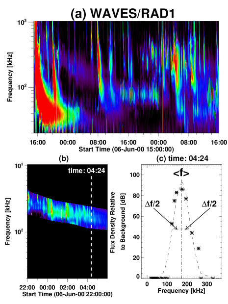
Figure 1.: Case study, central frequency and associated bandwidth deduction for event 1 (LASCO/CME on 6 June 2000). (a) WAVES/RAD1 dynamic spectrum associated with the propagation of the ICME/shock. (b) Isolated TII emission between 6-Jun-2000 22:00 UT to 7-Jun-2000 06:00 UT. (c) Flux density vs frequency for 1-min RAD1 spectrum at 04:24 UT. White dashed-line in panel (b) marks a temporal sample (at 04:24 UT) to perform the frequency analysis and the dashed black-line, in panel (c) points out the gaussian fit. Further description of the figure in the text.figure0

In practice, most observations of TII radio emissions are complex and show important fluctuations, and even gaps, in intensity, frequency emission and drift rate. Most of these fluctuations derive from the solar wind structure, the IP magnetic field topology and the shock front evolution [Knock and Cairns (2005)]. Due to such complexity, one of the problems in analysing TII emission is to identify the central emission frequency ($\langle f\rangle$) of the TII radio burst and the associated bandwidth ($\Delta f$). In order to simplify this task, we apply the technique by aguilar2005 and gonzalez2009 to infer $\langle f\rangle$ and its associated $\Delta f$. We present in Figure figure0 a case study to illustrate this technique. Figure figure0a shows the radio spectrum of event 1 (see Table tabla_eventos) detected by Radio Receiver Band 1 (RAD1) http://lep694.gsfc.nasa.gov/waves/data˙products.html. RAD1 is one of three radio receivers of the WAVES experiment on board the WIND spacecraft [Bougeret et al. (1995)]. RAD1 covers a frequency range from 20 to 1,040 kHz in a frequency band divided into 32 real channels. The frequency emission is observed at 15:00 UT on 6 June at 600 kHz, drifting slowly down to 60 kHz at 00:30 UT on 8 June. The TII emission is characterized by a single tone with intervals of very intense emission, which lasts several hours.

In Figure figure0b we isolated the TII event from the dynamic spectrum by setting to zero any emission outside the TII emission feature. Figure figure0b also shows a vertical dashed-line indicating a time sample (04:24 UT) on the TII emission. Figure figure0c shows this sample as a flux density vs frequency plot (asterisks), it also presents the Gaussian fit (dashed-line) to the flux-density distribution. This Gaussian approximation computes the values for $\langle f\rangle_{i}$ (dash-dotted line) and $\Delta f_{i}/2$ (dotted-lines) at the given time ($t_{i}$) (where $i$ is the index in the data series). The systematic repetition of this process, at every time sample of the spectrum, gives us also criteria to determine whether the time sample in the spectrum has a well-defined central emission or not (e.g., there are some spectra with multiple maxima in the flux density distribution, for these cases we discard the data point). After applying this filtering technique to the TII data, we obtain a set of $m$ values for $\langle f\rangle_{i}$, $\Delta f_{i}/2$ and $t_{i}$, with $1\leq i\leq m$.

corona2012c simulated TII emissions using a physical analytical model of ICMEs/shocks propagation. These synthetic radio bursts did not follow the central frequency of the associated TII emission but their lower frequency edge ($\underline{f}$). Assuming that the shock front is the TII source emission, the shock leading front is at the farthest distance from the Sun, which is associated with lower solar wind densities emitting at lower frequencies. Based on this previous experience, we will use the lower frequency edge ($\underline{f}$) of the TII emission for the regression model. From the analysis of radio data commented on before (see Figure figure0), we define the lower frequency edge as $\underline{f}_{i}=\langle f\rangle_{i}-\Delta f_{i}/2$. As we will explain below, with these frequency data we can reconstruct the trajectory of the IP shock.

2.2 Blast Wave Regression technique

technique2

The Blast Wave Regression (BWR) technique reconstructs the trajectory of shock fronts using TII data. In order to do so, this technique combines TII frequency data with the kinematic equations of a blast wave. A blast wave is a shock wave which has a finite amount of energy, the shock is transferring energy to the medium, decaying continuously as it propagates. In the case of an IP shock, a blast wave propagation implies that the shock decelerates following a particular rate [Rogers (1957)]. On the other hand, a driven shock is a shock wave that has a continuous source of energy from a driver, this source input energy replaces the energy that the shock transfers to the medium. In the case of an IP shock, a driven shock propagation implies that the shock and its driver (ICME) propagate at almost at almost the same speed [Parker (1961)]. Previous studies, using in situ data, suggest that IP shocks are not driven by their ICMEs further away from 1 AU [Burlaga et al. (1981), Feng et al. (2010)]. In fact, corona2011 claim that the CME/shock driven stage lasts just a few hours from which the IP shock propagation follows a blast wave decay. We should keep in mind, as commented on before, that the deceleration of fast CMEs/shocks in the IP medium is well established. For this study, we assume that IP shock waves follow a blast wave propagation from a certain heliocentric distance, which on average is about 15 R_⊙ (this value is obtained from the reconstruction algorithm).

cavaliere1976 investigated the self-similar solutions for shock waves propagating through different density profiles. According to them, when density decays as $r^{-2}$, the speed of a fast blast wave decreases as $(t/\tau)^{-1/3}$, with $\tau$ a constant of proportionality that modulates the decreasing rate of the shock speed. Furthermore, pinter1990 found that shock speed is convected by solar wind expansion. Thus, the speed ($v$) of an IP blast wave can be approximated by:

$$\ilabel{BWR_{v}}v=\left(v_{0}-w_{sw}\right)\left[\frac{t}{\tau}\right]^{-1/3}+w_{sw}\,,$$ (1)

where $v_{0}$ is the initial shock speed (at $t=\tau$) and $w_{sw}$ the solar wind speed. We can express the leading front position of a blast wave ($r$) by integrating Equation (BWR_v) over time:

$$\ilabel{BWR_{r}}r=w_{sw}\,t+\frac{3}{2}\tau^{1/3}\left(v_{0}-w_{sw}\right)t^{2/3}-\frac{1}{2}\left(v_{0}-w_{sw}\right)\tau+r_{0}\,,$$ (2)

with $r_{0}$ being an integration constant related with the initial position of the shock front (at $t=0$). Notice that Equations (BWR_v) and (BWR_r) are valid for $t\geq\tau$. In order to simplify the integration of Equation (BWR_v), we assumed $v=v_{0}$ for $0\leq t<\tau$.

Then, from the relation between plasma frequency, solar wind density and heliocentric distance, we can define the position of source region by:

$$\ilabel{SF_{r}}r_{i}=r(t_{i})=QN\sqrt{n_{1AU}}\frac{1}{\underline{f}_{i}}\,.$$ (3)

Where $n_{1AU}$ is the solar wind density at 1 AU and $Q=\sqrt{e^{2}(1{\rm AU})^{2}/4\pi^{2}\varepsilon_{0}m_{e}}$, with $e$, $\varepsilon_{0}$, and $m_{e}$ being the fundamental charge, electric constant and the electron mass, respectively. Additionally, $N$ indicates the fundamental frequency ($=1$) or the first harmonic ($=2$) and $\underline{f}$ is the lower frequency edge.

Now, by assuming that the location of TII source region is near the shock leading edge, we combine Equations (BWR_r) and (SF_r) to get:

$$\ilabel{BWR_{r}elation}\frac{1}{\underline{f}_{i}}=a_{3}t_{i}+a_{2}t_{i}^{2/3}+a_{0}\,.$$ (4)

Equation (BWR_relation) is a dispersion relation between frequencies and times that allows to reconstruct the kinematic evolution of IP shocks. The constants $a_{3}$, $a_{2}$ and $a_{0}$ are related with the blast wave equations by:

$$w_{sw} = a_{3}\sqrt{n_{1AU}}\,Q\,N\,,$$ (5)

$$\tau = \left[\frac{a_{3}r_{0}-a_{0}w_{sw}}{a_{2}w_{sw}}\right]^{3/2}\,,$$ (6)

$$v_{0} = w_{sw}\left(1+\frac{2a_{2}}{3a_{3}}\tau^{-1/3}\right)\,.$$ (7)

We calculate the values of $a_{3}$, $a_{2}$ and $a_{0}$ employing a gradient-expansion regression algorithm [Bevington and Robinson (2003)]. Using the regression algorithm we can describe the kinematics of shocks by Equations (BWR_v) and (BWR_r), as well as simulate the radio TII emission by combining Equations (SF_r) and (BWR_r). In the Appendix we present the relations to estimate uncertainties associated to the BWR technique.

3 Case events

results

We selected eight case events from the WIND/WAVES type II bursts and CMEs catalogue (http://cdaw.gsfc.nasa.gov/CME˙list/radio/waves˙type2.html) during the decaying phase of solar Cycle 23 (2000-2005). Table tabla_eventos shows the event list. In all cases, the associated TII emissions required to be clearly identified and to last several hours. All events were catalogued as halo CMEs (Earth-directed), with (plane-of-sky) initial speeds above 900 $kms^{-1}$ (Table tabla_eventos, column 3), and were associated with solar flares, as reported by SOHO LASCO CME [Gopalswamy et al. (2009)]. The flares’ locations were near the Sun’s center (see last column of Table tabla_eventos) to reduce possible directivity issues between the observer and TII source region. All the shocks and ICMEs were reported in richardson2010 catalogue, but event 4 which possibly was missed due to a data gap in ACE registers (see jian2006, catalog). We identified event 4 from WIND in situ data. Column 6 in Table tabla_eventos shows the transit times (from near the Sun to 1 AU) of shocks and ICMEs. Column 7 shows the speeds of shocks and ICMEs at 1 AU obtained from WIND data. We estimated the shock local speed at 1 AU ($v_{1AU}$), applying velocity coplanarity on the upstream and downstream in situ data. We calculated the ICME speed averaging WIND in situ data on the ejecta leading edge. Since there was a data gap in event 5 impeding the use of the velocity coplanarity to estimate the shock local speed, for this case, we used instead as a proxy the shock transit speed to 1 AU.

The first step in the methodology was to study 1-min resolution TII frequency data following the procedure described in Figure figure0. Subsequently, we reduced the frequency data temporal resolution to 0.5 hours, through an averaging process, in order to smooth out frequency irregularities to facilitate the convergence of the reconstruction algorithm. The averaging frequency data is presented in the bottom panels of Figures figure1 and figure2 as open-orange squares. Afterwards, we proceeded with the BWR technique by setting $r_{0}=6\,R_{\odot}$ (LASCO C2 external edge) for all the case events. The value of $n_{1AU}$ (see Table tabla_eventos, column 4) was taken from in situ measurements 8-12 hours before the shock arrival. The initially supplied function for the regression algorithm used $v_{0}=v_{cme0}$, $w_{sw}=w_{sw1}$ and $\tau=5\,r_{0}/v_{cme0}$ (see Table tabla_eventos). Additionally, we set $N=2$ for all the events (first harmonic frequency) and we used the detection time of each event as $t=0$ (Table tabla_eventos, column 2).

Events		Event data					Flare
#	Date-Houra	${v_{cme0}}^{a}$	${n_{1AU}}^{b}$	${w_{1AU}}^{b}$	$TT_{sh}$/$TT_{cme}$	${v_{1AU}}^{c}$/${v_{cme1AU}}^{d}$	Locatione-Classf
	[yyyymmdd]-[UT]	[$km~{}s^{-1}$]	[$cm^{-3}$]	[$km~{}s^{-1}$]	[$h$]	[$km~{}s^{-1}$]
1	20000606-15:54	1119	4.7	540	41.2/44.1	871/770	N20E18-X2.3
2	20000714-10:54	1674	3.5	700	27.5/31.9	1120/1040	N22W07-X5.7
3	20010426-12:30	1006	2.5	440	40.5/49.5	820/730	N20W05-M1.5
4	20010924-10:31	2402	3.2	590	34.5/39.0	641/530b	S16E23-X2.6
5	20011104-16:35	1810	7.5	420	33.5/34.9	g1206/750	N06W18-X1.0
6	20011122-23:30	1437	5.5	419	31.5/38.5	1108/1040	S17W36-M9.9
7	20040725-15:06	1333	1.8	599	31.9/35.1	1153/1000	N08W33-M1.1
8	20050513-17:12	1689	3.5	410	33.5/36.9	h1111/950	N12E11-M8.0
a SOHO LASCO CME catalog (http://cdaw.gsfc.nasa.gov/CME˙list/).
b Detected in situ by Wind (http://omniweb.gsfc.nasa.gov/).
c Calculated by velocity coplanarity.
d Taken from richardson2010 catalogue.
e SolarMonitor.org (http://www.solarmonitor.org/).
f NOAA classification.
g Estimated value $v_{1AU}=(1\,{\rm AU}-r_{0})/TT_{sh}$ due data gap.
h Value taken from bisi2010 due data gap.

Table 1.: List of events (chronograph and in situ measurements). From left to right: event number, date-time of CME detection, CME initial speed from LASCO observations; in situ values for proton density and bulk speed of solar wind; shock (/ICME) transit times and shock (/ICME) local speed at 1 AU; and location (-class) of the associated solar flare.tabla˙eventos

3.1 Results

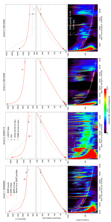
Figure 2.: Analysis results for events 1-4. Each column presents the results for one single event, while the rows present (from top to bottom) the results and data of speed, heliocentric distance and the dynamic radio spectrum, respectively. In upper and middle panels the open-diamonds, open-stars, asterisks and down-ward open-triangles represent different data. Due to space constrains, the references for the symbols and line styles in the two top rows are spread among the top panels. Solid-lines represent the shock trajectory obtained by the BWR technique. The IPS velocity data is from STEL as reported by Gonzalez-Esparza and Aguilar-Rodriguez (2009). In the bottom panels, open orange-squares point out the averaging type II frequency data. See the text for further description. figure1

We present the results of the case events in Figures figure1 and figure2. In both figures, each column represents a single event, meanwhile the rows, from top to bottom, show the speed and heliocentric distance of the shock fronts in time and the dynamic radio spectra. The vertical dash-dotted lines point out the event detection-time reported by LASCO CME catalogue (see Table tabla_eventos, column 1). Upper and middle panels of the figures present the shock trajectories (speed and position versus time) obtained from the BWR technique (solid-red lines). In the panels, we point out the initial (fill circles) and final (open circles) parameters calculated by the BWR technique. In these panels, for comparison with the BWR results, we also present data from: coronagraph images (open-diamonds) as reported by SOHO LASCO CME [Gopalswamy et al. (2009)] catalog; in situ data of ICME (down-ward open-triangles) and shock (asterisks) arrivals at 1 AU; and IPS speed measurements (open-stars) as reported by gonzalez2009 and bisi2010. In the bottom panels of the figures, we overplot the simulated radio emission (solid-white line) obtained from the BWR technique as well the radio data used in our analysis (open orange-squares).

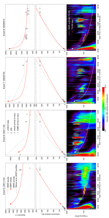
Figure 3.: Analysis results for events 5-8. Description is the same as Figure figure1. The IPS velocity data is from STEL and ORT (2005/05/13) as reported by Gonzalez-Esparza and Aguilar-Rodriguez (2009) and Bisi et.al. (2010).figure2

In most cases, the simulated radio emission approximates very well the frequency data. For events 6 and 7 (Figure figure2) the limited TII data derived into poor BWR results. However, it is remarkable that, despite the limitation in the TII data, it was possible to apply the BWR technique in both events. Furthermore, in all cases the simulated frequency drift systemically limit the lower edge of the observed TII radio emission.

Event	BWR results							$\alpha$
#	$\tau(r_{\tau})^{a}$	$w_{0}$	$v_{0}$	$TT_{sh}$	$v_{1AU}$	Differences [$\%$]
	[$h$]([$R_{\odot}$])	[$km~{}s^{-1}$]	[$km~{}s^{-1}$]	[$h$]	[$km~{}s^{-1}$]	$TT_{sh}$([$h$])	$v_{1AU}$	[∘]
1	1.00(14.0)	540	1542	42.1	828	2.2 (+0.9)	4.9	27
2	0.67(14.3)	700	2387	28.9	1180	5.1 (+1.4)	5.4	23
3	1.11(14.1)	440	1420	47.6	720	17.5 (+7.1)	12.2	21
4	2.30(27.9)	317	1840	33.7	940	2.3 (-0.8)	46.6	28
5	4.08(42.6)	543	1733	29.2	1160	b12.8 (-4.3)	b3.8	19
6	2.68(27.1)	429	1522	37.9	881	20.3 (+6.4)	20.5	39
7	0.84(14.1)	599	1870	35.8	962	12.8 (+4.1)	16.6	34
8	0.66(15.0)	410	2625	30.9	1024	7.8 (-2.6)	7.8	16
Averages	1.67(21.1)	497	1867	35.8	908	10.0 (c3.5)	13.7	26
							d9.0
a Heliocentric distance at $\tau$, $r_{\tau}=r_{0}+v_{0}\,\tau$.
b Estimated value due data gap.
c Absolute average.
d By neglecting event 4.

Table 2.: Results from BWR analysis. From left to right: event number; values of $\tau$ and associated heliocentric distance ($r_{\tau}$), calculated value of the ambient solar wind ($w_{sw}$), calculated value of the shock initial speed ($v_{0}$); calculated shock transit time ($TT_{sh}$); calculated shock local speed at 1 AU ($v_{1AU}$); proportional absolute difference between calculated and in situ registered values of $TT_{sh}$ and $v_{1AU}$; and angle ($\alpha$) between Sun-Earth line and location of associated solar flare. Column 7 also shows the direct difference between calculated and in situ registered values of $TT_{sh}$.tabla˙resultados

In general, the resulting trajectories (position and speeds) are in good agreement with coronagraph, IPS and in situ measurements. Table tabla_resultados summarizes the main results of the analysis of the 8 case events, comparing the BWR calculations with coronograph and in situ data (Table 1). According to Equations (BWR_r) and (BWR_v), the calculated trajectory of the shock starts at $t=\tau$, time at which begins the shock blast wave propagation (Column 2). In general, the calculated shock initial positions ($t\sim\tau$) were located within the coronagraph (LASCO-C3) field of view. The calculated shock transit times (column 5) were quantitatively consistent with the in situ arrivals of the IP shocks. Column 7 lists the relative differences between calculated and in situ measurement of shock transit times ($TT$), where the average difference is about 10%. Column 8 lists the relative differences between calculated and in situ measurement of shock speed at 1 AU ($v_{1AU}$). The average relative normalized difference was about 14%. Note that the difference for event 4 is the largest; however, in this case, the estimation of the in situ shock speed has a large uncertainty. The fourth row of Figure figure1 (upper panel) shows the largest error in the shock speed estimation. Neglecting event 4, the average associated difference of shock local speeds drops to 9% (similar to the one for $TT_{sh}$).

The BWR calculations of the shock speed evolution in Figures figure1 and figure2 (upper panels) present an initial strong deceleration that rapidly decreases with time. Such deceleration considerably reduces ($\sim\,50\%$) the speed of IP shocks when they arrive to 1 AU (see Table tabla_resultados, columns 3 and 5). However, note that the deceleration is different for each event. We can estimate the decaying rate of shock speed by Equation (BWR_v):

$$\frac{dv}{dt}=-\frac{a_{0}}{3}\left(\frac{t}{\tau}\right)^{-3/4}\,,$$

where $a_{0}=[v_{0}-w_{sw}]/\tau$ can be interpreted as an effective acceleration. Then, larger values of $a_{0}$, imply stronger decelerations acting on blast waves. Events 2 and 8 exemplify the effects of different values of $v_{0}-w_{sw}$ with similar $\tau$. For event 2 ($a_{0}=699\,ms^{-2}$) the decrease in speed at 1 AU was $\sim 50\%$; whereas for event 8 ($a_{0}=932\,ms^{-2}$) it was $\sim 61\%$. On the other hand, events 5 and 6 show the case for different values of $\tau$ and close values of $v_{0}-w_{sw}$. For event 5 ($a_{0}=81\,ms^{-2}$) the shock speed decreases $\sim 33\%$; whereas in event 6 ($a_{0}=113\,ms^{-2}$) the reduction was $\sim 42\%$.

The BWR calculated shock parameters at 1 AU for events 3, 5, 6 and 7 present differences with in situ data. Such differences may derive from contamination of the TII radio spectrum and/or directivity issues. On one hand, events 3 and 5 occurred during high solar activity intervals with occurrence of other CMEs before and after. This could lead into multiple (complex) CMEs propagating through an unstable ambient solar wind. This scenario might contaminate the TII dynamic radio spectra, misleading the results. On the other hand, the associated-flare locations of events 6 and 7 have a large angular distance ($\sim 35^{\circ}$) with respect to the Sun-Earth line (see Table tabla_resultados, column 8). Using the flare location as a proxy for the CME propagation direction, we can estimate if the source emission is propagating far away from the Sun-Earth line. For these cases, the radio source may not be directly seen by the observer. TII emissions are affected by the line of sight between the observer and the source [Knock and Cairns (2005)]. This might be the case in event 7, where the TII emission does not appear as a continuous frequency drift, but like a chain of consecutive bursts. For events 6 and 7, this directivity issue might explain the reduced number of TII radio data, resulting into poor BWR results. In Figure figure2 the simulated TII emission of events 6 and 7 barely follows the TII spectral data.

4 Discussion

discussion

We present the BWR technique to reconstruct the evolution of shock fronts using TII emission data. The technique is based on three main assumptions: (1) solar wind density decays as $r^{-2}$ and expands with constant speed ($w_{sw}$); (2) the TII emission source is located somewhere near the leading edge of the shock front; and (3) IP shocks evolve as blast waves. According to the first assumption, this technique would be more suitable for quiet periods of solar activity, when isolated fast CME events propagate through a quasi-stationary ambient solar wind. On the other hand, note that the average initial positions of blast wave propagation ($r_{\tau}$), given by the BWR results, were located around $21\,R_{\odot}$ (see Table tabla_resultados column 2) which is beyond the supermagnetosonic point.

With respect to the second assumption, as some authors suggest, the source region of TII emissions might be located far from the shock’s leading edge [Knock et al. (2003)]. This source location may affect the results of this technique. The two events in the list whose associated flare locations were more than $30^{\circ}$ from the Sun center (events 6 and 7 in the last column of Table 2) had significant differences with respect to the in situ measurements. It is possible that these errors were related to the location of the source regions, and that the BWR technique is more suitable for Earth-directed events, where source regions are close to the Sun-Earth line.

It is not clear where ICMEs get exhausted of driving IP shocks in the inner heliosphere. However, beyond that critical distance ($r_{\tau}$), the IP shocks should evolve as blast waves, as the third assumption dictates. As commented in the Introduction, there are multiple works that suggest that IP shocks evolve as blast waves. For example, burlaga1981, by analyzing ICMEs/shocks detected by Voyager 1 and 2, found that the shock might be no longer driven by ICMEs at heliocentric distances around 2 AU. Departing from geometrical analysis, feng2010 found that at least $34\%$ of shocks detected in situ (at 1 AU) were not driven by their associated ICMEs. corona2011 studied the momentum fluxes between ICMEs and plasma sheaths using numerical simulations and concluded that IP shocks are no longer driven by ICMEs when they reach 1 AU. The results from our study suggest that IP shocks evolve as blast waves beyond $\sim 21\,R_{\odot}$ ($t>\tau$). This value is consistent with the ones separately found by pinter1990 ($\sim 0.12\,{\rm AU}=25.8\,R_{\odot}$) and corona2012c ($\sim 44.7\,R_{\odot}$) through empirical and analytic approaches, respectively. Furthermore, by assuming blast wave propagation for IP shocks, the BWR technique was able to reconstruct speed and position profiles that showed qualitative and quantitative agreements with a number of different data. Furthermore, blast wave propagation explains the well known fact of deceleration of IP shocks, as well as the unexpected growth in stand-off distances found by maloney2011.

In Figures 2 and 3 (upper and middle panels) we plot the shock trajectories using the approximation by reiner2007 (dotted grey line). They proposed a two stages kinematic model to proxy the trajectory of fast ICMEs/shocks. Such a model consists in a pristine period of intense deceleration followed by a constant speed stage. Then they search for the trajectories of ICME/shocks that simultaneously satisfied data from coronagraph images, in situ registers and TII emissions. Comparing our solutions with the ones obtained by reiner2007, we notice similarities between them. Blast wave speeds present an initial strong deceleration which rapidly decreases with time. This behavior resembles the one presented by the two stages kinematic model. Event 1 is an example where there is a good agreement between the two methodologies which both predict very similar shock arrival times to 1 AU.

Though BWR technique is presented as a tracking method for IP shocks; it might be useful for forecasting proposes. According to our results, BWR is more suitable, but not restricted, for Earth-directed shocks occurring during quiet periods of solar activity. Our calculated shock trajectories showed a tendency to arrive later than their in situ counterparts. The average difference between calculated and in situ-registered transit times was 3.5 h, a value similar to others ($\sim 7\,{\rm h}$) derived from empirical (e.g. cremades2007; feng2009; mostl2011) and analytical (e.g. feng2006; song2010) arrival-predicting tools. An important limitation of BWR technique, for predicting proposes, is the acquisition of in situ data. This data is taken around 8-12 hours before shock arrival, leaving few hours to issue alarms. Though this limitation can be easily solved by using IPS measurements or average values of solar wind density at 1 AU, exploring this topic escapes the scopes of this work.

The BWR calculated shock speed profiles were consistent with coronagraph, in situ and IPS data. However, although our results showed good agreement with different data, we have to point out that those data correspond to different but related structures. On one hand, coronagraph images give information about (plane-of-sky) propagation of CMEs in the solar corona. On the other hand, IPS speeds might be related to plasma sheaths behind the IP shocks, and the in situ measurements to local characteristics of ICMEs and shocks at 1 AU.

The BWR technique is sensitive to contamination and directivity issues on TII emission data. The applicability of BWR, and the certainty on its results, will depend on the availability and quality of the TII data. However, the calculated transit times and arrival speeds of shocks were quantitatively consistent with their in situ registered counterparts. In average, our results showed $\sim 90\%$ of agreement with in situ data (see Table tabla_resultados, column 7). Even for unfavorable events (say events 3, 5, 6, 7), it was possible to approximate $TT_{sh}$ and $v_{1AU}$ with reasonable agreement with the in situ data.

5 Conclusions

conclusions

We introduced the blast wave regression (BWR) technique. This technique reconstructs the evolution of fast ICMEs/shocks associated with type II radio bursts. The technique assumes that interplanetary shocks propagate as blast waves through a stationary homogeneous ambient solar wind, whose density decays with the square of the heliocentric distance. Using frequency data from the TII emission, the technique develops a dispersion relation whose regression solves the kinematics (speed and position) of the IP shock. We applied the BWR technique to analyze 8 ICME/shock events associated with TII emissions occurred during the decaying phase of solar cycle 23. The results suggest that the shock events propagated as blast waves beyond $\sim 21\,R_{\odot}$. The BWR results also showed notable consistencies with data from coronagraph images, speeds deduced from IPS observations and in situ measurements. The BWR calculated transit times and arrival speeds (at 1 AU) of shocks showed about $90\%$ of consistency with the in situ data. The accuracy of this technique depends on the availability and quality of the type II spectral data associated with the ICME/shock. The results may be mislead by contamination of radio data and directivity issues. However, even for those unfavorable conditions, the technique was capable to estimate transit times and arrival speeds that differed around $20\%$ from their in situ counterparts. The agreement that our results showed with different data sets, preliminarily indicates that the BWR technique could be a useful tool for ICME/shock tracking and arrival forecasting, although the performance analysis of the latter is not under the scope of this paper.

apendice

Uncertainties

We can estimate the uncertainties associated with the BWR technique by using the differentiation method. Then, the uncertainty ($\delta r_{i}$) of $r_{i}$ is given by:

$$\ilabel{SF_{d}r}\frac{\delta r_{i}}{r_{i}}=\frac{\delta n_{1AU}}{n_{1AU}}+\frac{\delta\underline{f}_{i}}{\underline{f}_{i}}\,,$$ (8)

where $\delta n_{1AU}$ and $\underline{f}_{i}$ are the uncertainties of $n_{1AU}$ and $\underline{f}_{i}$, respectively. Here we can estimate $\delta\underline{f}_{i}\sim\Delta f_{i}/4$. Finally, the uncertainties on shock trajectory are expressed by:

$$\frac{\delta w_{sw}}{w_{sw}} = \frac{\delta n_{1AU}}{2n_{1AU}}\,,$$ (9)

$$\frac{\delta\tau}{\tau} = \frac{3}{2}\left[\frac{a_{3}\delta r_{0}-a_{0}\delta w_{sw}}{a_{3}r_{0}-a_{0}w_{sw}}+\frac{\delta w_{sw}}{w_{sw}}\right]\;{\rm and}$$ (10)

$$\frac{\delta v_{0}}{v_{0}} = \frac{\delta w_{sw}}{w_{sw}}+\left[\frac{2a_{2}}{9a_{3}\tau^{1/3}+6a_{2}}\right]\frac{\delta\tau}{\tau}\,.$$ (11)

Where $\delta w_{sw}$, $\delta\tau$ and $\delta v_{0}$ are the errors of solar wind speed, $\tau$ and initial speed of shock front, respectively. Additionally, $\delta n_{1AU}$ is the uncertainty related to $n_{1AU}$ and $\delta r_{0}$ the uncertainty of $r_{0}$.

Acknowledgements

P. Corona-Romero, V. De-la-Luz and J.C. Mejia-Ambriz thanks Catedras-CONACyT project 1045: Servicio de Clima Espacial Mexico (SCiESMEX). J. A. Gonzalez.-Esparza acknowledges the partial funding by the DGAPA-PAPIIT grant IN109413 and CONACyT grant 152471. E. Aguilar-Rodriguez thanks DGAPA-PAPIIT grant IN103615, and CONACyT grant 220981.

References

- Aguilar-Rodriguez et al. (2005) Aguilar-Rodriguez, E., Gopalswamy, N., MacDowall, R., Yashiro, S., Kaiser, M.L.: 2005, A universal characteristic of type II radio bursts. Journal of Geophysical Research (Space Physics) 110, 12. doi:10.1029/2005JA011171.
- Bevington and Robinson (2003) Bevington, P.R., Robinson, D.K.: 2003, Data reduction and error analysis for the physical sciences.
- Bisi et al. (2010) Bisi, M.M., Breen, A.R., Jackson, B.V., Fallows, R.A., Walsh, A.P., Mikić, Z., Riley, P., Owen, C.J., Gonzalez-Esparza, A., Aguilar-Rodriguez, E., Morgan, H., Jensen, E.A., Wood, A.G., Owens, M.J., Tokumaru, M., Manoharan, P.K., Chashei, I.V., Giunta, A.S., Linker, J.A., Shishov, V.I., Tyul’Bashev, S.A., Agalya, G., Glubokova, S.K., Hamilton, M.S., Fujiki, K., Hick, P.P., Clover, J.M., Pintér, B.: 2010, From the Sun to the Earth: The 13 May 2005 Coronal Mass Ejection. Solar Physics 265, 49 – 127. doi:10.1007/s11207-010-9602-8.
- Bougeret et al. (1995) Bougeret, J.-L., Kaiser, M.L., Kellogg, P.J., Manning, R., Goetz, K., Monson, S.J., Monge, N., Friel, L., Meetre, C.A., Perche, C., Sitruk, L., Hoang, S.: 1995, Waves: The Radio and Plasma Wave Investigation on the Wind Spacecraft. Space Science Reviews 71, 231 – 263. doi:10.1007/BF00751331.
- Burlaga et al. (1981) Burlaga, L., Sittler, E., Mariani, F., Schwenn, R.: 1981, Magnetic loop behind an interplanetary shock - Voyager, Helios, and IMP 8 observations. Journal of Geophysical Research 86, 6673 – 6684. doi:10.1029/JA086iA08p06673.
- Cane and Stone (1984) Cane, H.V., Stone, R.G.: 1984, Type II solar radio bursts, interplanetary shocks, and energetic particle events. Astrophysical Journal 282, 339 – 344. doi:10.1086/162207.
- Cane, Sheeley, and Howard (1987) Cane, H.V., Sheeley, N.R. Jr., Howard, R.A.: 1987, Energetic interplanetary shocks, radio emission, and coronal mass ejections. Journal of Geophysical Research 92, 9869 – 9874. doi:10.1029/JA092iA09p09869.
- Cavaliere and Messina (1976) Cavaliere, A., Messina, A.: 1976, Propagation of blast waves. Astrophysical Journal 209, 424 – 428. doi:10.1086/154736.
- Corona-Romero and Gonzalez-Esparza (2011) Corona-Romero, P., Gonzalez-Esparza, J.A.: 2011, Numeric and analytic study of interplanetary coronal mass ejection and shock evolution: Driving, decoupling, and decaying. Journal of Geophysical Research (Space Physics) 116, 5104. doi:10.1029/2010JA016008.
- Corona-Romero, Gonzalez-Esparza, and Aguilar-Rodriguez (2013) Corona-Romero, P., Gonzalez-Esparza, J.A., Aguilar-Rodriguez, E.: 2013, Propagation of Fast Coronal Mass Ejections and Shock Waves Associated with Type II Radio-Burst Emission: An Analytic Study. Solar Physics 285, 391 – 410. doi:10.1007/s11207-012-0103-9.
- Cremades, St. Cyr, and Kaiser (2007) Cremades, H., St. Cyr, O.C., Kaiser, M.L.: 2007, A tool to improve space weather forecasts: Kilometric radio emissions from Wind/WAVES. Space Weather 5, 8001. doi:10.1029/2007SW000314.
- Dryer (1974) Dryer, M.: 1974, Interplanetary Shock Waves Generated by Solar Flares. Space Science Reviews 15, 403 – 468. doi:10.1007/BF00178215.
- Dryer and Smart (1984) Dryer, M., Smart, D.F.: 1984, Dynamical models of coronal transients and interplanetary disturbances. Advances in Space Research 4, 291 – 301. doi:10.1016/0273-1177(84)90573-8.
- Feng et al. (2010) Feng, H.Q., Wu, D.J., Chao, J.K., Lee, L.C., Lyu, L.H.: 2010, Are all leading shocks driven by magnetic clouds? Journal of Geophysical Research (Space Physics) 115, 4107. doi:10.1029/2009JA014875.
- Feng et al. (2009) Feng, X.S., Zhang, Y., Sun, W., Dryer, M., Fry, C.D., Deehr, C.S.: 2009, A practical database method for predicting arrivals of “average” interplanetary shocks at Earth. Journal of Geophysical Research (Space Physics) 114, 1101. doi:10.1029/2008JA013499.
- Feng and Zhao (2006) Feng, X., Zhao, X.: 2006, A new prediction method for the arrival time of interplanetary shocks. Solar Physics 238, 167 – 186.
- Gonzalez-Esparza and Aguilar-Rodriguez (2009) Gonzalez-Esparza, A., Aguilar-Rodriguez, E.: 2009, Speed evolution of fast CME/shocks with SOHO/LASCO, WIND/WAVES, IPS and in-situ WIND data: analysis of kilometric type-II emissions. Annales Geophysicae 27, 3957 – 3966. doi:10.5194/angeo-27-3957-2009.
- Gopalswamy et al. (2000) Gopalswamy, N., Lara, A., Lepping, R.P., Kaiser, M.L., Berdichevsky, D., St. Cyr, O.C.: 2000, Interplanetary acceleration of coronal mass ejections. Geophysical Research Letters 27, 145 – 148. doi:10.1029/1999GL003639.
- Gopalswamy et al. (2005) Gopalswamy, N., Lara, A., Manoharan, P.K., Howard, R.A.: 2005, An empirical model to predict the 1-AU arrival of interplanetary shocks. Advances in Space Research 36, 2289 – 2294. doi:10.1016/j.asr.2004.07.014.
- Gopalswamy et al. (2008) Gopalswamy, N., Yashiro, S., Akiyama, S., Mäkelä, P., Xie, H., Kaiser, M.L., Howard, R.A., Bougeret, J.L.: 2008, Coronal mass ejections, type II radio bursts, and solar energetic particle events in the SOHO era. Annales Geophysicae 26, 3033 – 3047. doi:10.5194/angeo-26-3033-2008.
- Gopalswamy et al. (2009) Gopalswamy, N., Yashiro, S., Michalek, G., Stenborg, G., Vourlidas, A., Freeland, S., Howard, R.: 2009, The SOHO/LASCO CME Catalog. Earth Moon and Planets 104, 295 – 313. doi:10.1007/s11038-008-9282-7.
- Gosling et al. (1968) Gosling, J.T., Asbridge, J.R., Bame, S.J., Hundhausen, A.J., Strong, I.B.: 1968, Satellite observations of interplanetary shock waves. Journal of Geophysical Research 73, 43. doi:10.1029/JA073i001p00043.
- Jian et al. (2006) Jian, L., Russell, C.T., Luhmann, J.G., Skoug, R.M.: 2006, Properties of Interplanetary Coronal Mass Ejections at one AU during 1995-2004. Solar Physics 239, 393.
- Knock and Cairns (2005) Knock, S.A., Cairns, I.H.: 2005, Type II radio emission predictions: Sources of coronal and interplanetary spectral structure. Journal of Geophysical Research (Space Physics) 110, 1101. doi:10.1029/2004JA010452.
- Knock et al. (2003) Knock, S.A., Cairns, I.H., Robinson, P.A., Kuncic, Z.: 2003, Theoretically predicted properties of type II radio emission from an interplanetary foreshock. Journal of Geophysical Research (Space Physics) 108, 1126. doi:10.1029/2002JA009508.
- Leblanc et al. (2001) Leblanc, Y., Dulk, G.A., Vourlidas, A., Bougeret, J.-L.: 2001, Tracing shock waves from the corona to 1 AU: Type II radio emission and relationship with CMEs. Journal of Geophysical Research 106, 25301 – 25312. doi:10.1029/2000JA000260.
- Lindsay et al. (1999) Lindsay, G.M., Luhmann, J.G., Russell, C.T., Gosling, J.T.: 1999, Relationships between coronal mass ejection speeds from coronagraph images and interplanetary characteristics of associated interplanetary coronal mass ejections. Journal of Geophysical Research 104, 12515 – 12524. doi:10.1029/1999JA900051.
- Maloney and Gallagher (2011) Maloney, S.A., Gallagher, P.T.: 2011, STEREO Direct Imaging of a Coronal Mass Ejection-driven Shock to 0.5 AU. Astrophysical Journal Letters 736, L5. doi:10.1088/2041-8205/736/1/L5.
- Möstl et al. (2011) Möstl, C., Rollett, T., Lugaz, N., Farrugia, C.J., Davies, J.A., Temmer, M., Veronig, A.M., Harrison, R.A., Crothers, S., Luhmann, J.G., Galvin, A.B., Zhang, T.L., Baumjohann, W., Biernat, H.K.: 2011, Arrival Time Calculation for Interplanetary Coronal Mass Ejections with Circular Fronts and Application to STEREO Observations of the 2009 February 13 Eruption. Astrophysical Journal 741, 34. doi:10.1088/0004-637X/741/1/34.
- Ontiveros and Gonzalez-Esparza (2010) Ontiveros, V., Gonzalez-Esparza, J.A.: 2010, Geomagnetic storms caused by shocks and ICMEs. Journal of Geophysical Research (Space Physics) 115, 10244. doi:10.1029/2010JA015471.
- Parker (1961) Parker, E.N.: 1961, Sudden Expansion of the Corona Following a Large Solar Flare and the Attendant Magnetic Field and Cosmic-Ray Effects. Astrophysical Journal 133, 1014. doi:10.1086/147105.
- Pinter (1982) Pinter, S.: 1982, Experimental study of flare-generated collisionless interplanetary shock wave propagation. Space Science Reviews 32, 145 – 168. doi:10.1007/BF00225182.
- Pinter and Dryer (1985) Pinter, S., Dryer, M.: 1985, The influence of the energy emitted by solar flare soft X-ray bursts on the propagation of their associated interplanetary shock waves. Astrophysics and Space Science 116, 51 – 60. doi:10.1007/BF00649273.
- Pinter and Dryer (1990) Pinter, S., Dryer, M.: 1990, Conversion of piston-driven shocks from powerful solar flares to blast waves in the solar wind. Bulletin of the Astronomical Institutes of Czechoslovakia 41, 137 – 148.
- Reiner, Kaiser, and Bougeret (2007) Reiner, M.J., Kaiser, M.L., Bougeret, J.-L.: 2007, Coronal and Interplanetary Propagation of CME/Shocks from Radio, In Situ and White-Light Observations. Astrophysical Journal 663, 1369 – 1385. doi:10.1086/518683.
- Richardson and Cane (2010) Richardson, I.G., Cane, H.V.: 2010, Near-Earth Interplanetary Coronal Mass Ejections During Solar Cycle 23 (1996 - 2009): Catalog and Summary of Properties. Solar Physics 264, 189 – 237. doi:10.1007/s11207-010-9568-6.
- Rogers (1957) Rogers, M.H.: 1957, Analytic Solutions for the Blast-Wave Problem with an Atmosphere of Varying Density. Astrophysical Journal 125, 478. doi:10.1086/146323.
- Rogers (1958) Rogers, M.H.: 1958, Similarity flows behind strong shock waves. The Quarterly Journal of Mechanics and Applied Mathematics 11(4), 411 – 422.
- Smart and Shea (1985) Smart, D.F., Shea, M.A.: 1985, A simplified model for timing the arrival of solar flare-initiated shocks. Journal of Geophysical Research 90, 183 – 190. doi:10.1029/JA090iA01p00183.
- Song (2010) Song, W.B.: 2010, An Analytical Model to Predict the Arrival Time of Interplanetary CMEs. Solar Physics 261, 311 – 320. doi:10.1007/s11207-009-9486-7.
- Vourlidas et al. (2003) Vourlidas, A., Wu, S.T., Wang, A.H., Subramanian, P., Howard, R.A.: 2003, Direct Detection of a Coronal Mass Ejection-Associated Shock in Large Angle and Spectrometric Coronagraph Experiment White-Light Images. Astrophysical Journal 598, 1392 – 1402. doi:10.1086/379098.
- Watari and Detman (1998) Watari, S., Detman, T.: 1998, In situ local shock speed and transit shock speed. Annales Geophysicae 16, 370 – 375. doi:10.1007/s00585-998-0370-9.