Facets of the Balanced Minimal Evolution Polytope.

Abstract.

The balanced minimal evolution (BME) method of creating phylogenetic trees can be formulated as a linear programming problem, minimizing an inner product over the vertices of the BME polytope. In this paper we undertake the project of describing the facets of this polytope. We classify and identify the combinatorial structure and geometry (facet inequalities) of all the facets in dimensions up to 5, and classify even more facets in all dimensions. A full set of facet inequalities would allow a full implementation of the simplex method for finding the BME tree–although there are reasons to think this an unreachable goal. However, our results provide the crucial first steps for a more likely-to-be-successful program: finding efficient relaxations of the BME polytope.

1. Introduction

Figure 1. There are two combinatorial types of facets of the 5-dimensional BME polytope, shown here as Schlegel diagrams. The polytope on the left is the 4-simplex, and on the right is the 4d Birkhoff polytope. The Schlegel diagram for the latter is expanded in Figure 11.

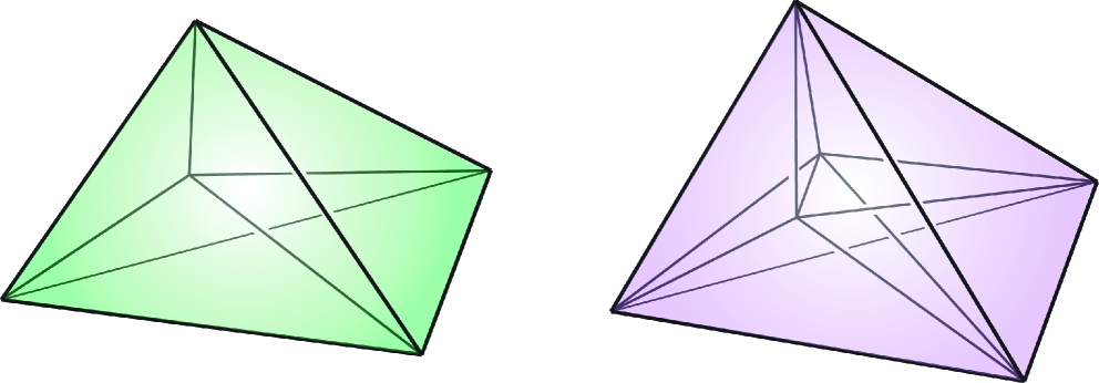
The goal of phylogenetics is to take a set of related items– biological examples are usually referred to as taxa: populations, species, individuals or genes–and to construct a branching diagram that explains how they are related chronologically. The diagram we will be concerned with is a binary tree with labeled leaves. In other words, a cycle-free graph with nodes (vertices) which are either of degree one (touching a single edge) or degree three, and with a set of distinct items assigned to the degree one nodes–the leaves. We study a method called balanced minimal evolution. This method begins with a given set of $n$ items and a symmetric (or upper triangular) square $n\times n$ dissimilarity matrix whose entries are numerical dissimilarities, or distances, between pairs of items. From the dissimilarity matrix the balanced minimal evolution (BME) method constructs a binary tree with the $n$ items labeling the $n$ leaves. The BME tree has the property that the distances between its leaves most closely match the given distances between corresponding pairs of taxa.

By “most closely match” in the previous paragraph we mean the following: the reciprocals of the distances between leaves are the components of a vector $\mathbf{c}$, and this vector minimizes the dot product $\mathbf{c}\cdot\mathbf{d}$ where $\mathbf{d}$ is the list of distances in the upper triangle of the distance matrix.

More precisely: Let the set of $n$ distinct species, or taxa, be called $S.$ For convenience we will often let $S=[n]=\{1,2,\dots,n\}.$ Let vector $\mathbf{d}$ be given, having ${n\choose 2}$ real valued components $d_{ij}$, one for each pair $\{i,j\}\subset S.$ There is a vector $\mathbf{c}(t)$ for each binary tree $t$ on leaves $S,$ also having ${n\choose 2}$ components $c_{ij}(t)$, one for each pair $\{i,j\}\subset S.$ These components are ordered in the same way for both vectors, and we will use the lexicographic ordering: $\mathbf{d}=\left<d_{12},d_{13},\dots,d_{1n},d_{23},d_{24},\dots,d_{n-1,n}\right>$.

We define, following Pauplin [Pau00]:

$$c_{ij}(t)=\frac{1}{2^{l}}$$

where $l$ is the number of internal nodes (degree 3 vertices) in the path from leaf $i$ to leaf $j.$

The BME tree for the vector $\mathbf{d}$ is the binary tree $t$ that minimizes $\mathbf{d}\cdot\mathbf{c}(t)$ for all binary trees on leaves $S.$ The value of setting up the question in this way is that it becomes a linear programming problem. The convex hull of all the vectors $\mathbf{c}(t)$ for all binary trees $t$ on $S$ is a polytope BME$(S)$, hereafter also denoted BME($n$) or $\mathcal{P}_{n}$ as in [EHPY08] and [HHY11]. The vertices of $\mathcal{P}_{n}$ are precisely the $(2n-5)!!$ vectors $\mathbf{c}(t).$ Minimizing our dot product over this polytope is equivalent to minimizing over the vertices, and thus amenable to the simplex method.

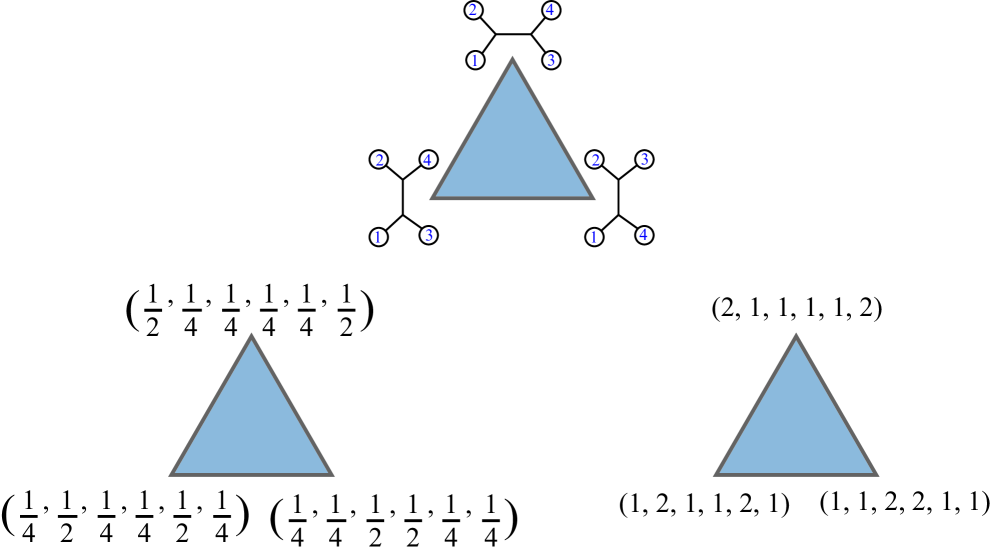
In Figure 2 we see the 2-dimensional polytope $\mathcal{P}_{4}.$ In that figure we illustrate a simplifying choice that will be used throughout: rather than the original fractional coordinates $c_{ij}$ we will scale by a factor of $2^{n-2},$ giving coordinates $x_{ij}=2^{n-2}c_{ij}=2^{n-2-l}.$ Since the furthest apart any two leaves may be is a distance of $n-2$ internal nodes, this scaling will result in integral coordinates.

Figure 2. The polytope $\mathcal{P}_{4}$ is a triangle. At the top we label the vertices with the three binary trees with leaves $1\dots 4$. Each edge shows a nearest-neighbor interchange; for instance the exchange of leaves 3 and 4 on the bottom edge. At bottom left are Pauplin’s original coordinates and at bottom right are the coordinates, scaled by $2^{n-2}=4$, which we will use.

A clade is a subgraph of a binary tree induced by an internal (degree three) node and all of the leaves descended from it in a particular direction. In other words: given an internal node $v$ we choose two of its edges and all of the leaves that are connected to $v$ via those two edges. Equivalently, given any internal edge, its deletion separates the tree into two clades. Two clades on the same tree must be either disjoint or nested, one contained in the other. A cherry is a clade with two leaves. We often refer to a clade by its set of (2 or more) leaves. A pair of intersecting cherries $\{a,b\}$ and $\{b,c\}$ have intersection in one leaf $b$, and thus cannot exist both on the same tree. A caterpillar is a tree with only two cherries.

2. New Results

A facet of a polytope is a top-dimensional face of that polytope’s boundary, or a co-dimension-1 face. Faces of a polytope can be of any dimension, from 0 to that of the (improper) face which is the polytope itself. Our main results are to describe many new faces, especially facets, of the $n^{th}$ balanced minimal evolution polytope $\mathcal{P}_{n}$.

For $n=5$ we completely classify the facets according to combinatorial type of their vertices. There are three classes of facet for $n=5$, which we refer to as intersecting-cherry facets, caterpillar facets, and cyclic-ordering facets. There are respectively 30, 10 and 12 of these types of facet in $\mathcal{P}_{5}.$

In Theorem 4.3 we show that any pair of intersecting cherries corresponds to a facet of $\mathcal{P}_{n}.$ In Theorem 4.1 we (redundantly, for demonstrative purpose) show a special case of this facet for $n=5$ and in Theorem 4.2 we show that for $n=5$ these facets turn out to be equivalent to Birkhoff polytopes.

In Theorem 6.3 we show that any caterpillar tree with fixed ends corresponds to a facet of $\mathcal{P}_{n}.$ For $n=5$ we show in Theorem 6.2 that this facet is a Birkhoff polytope.

In Theorem 5.1 we show that, for $n=5,$ for each free cyclic ordering of leaves there is a corresponding facet which is combinatorially equivalent to a simplex.

The right half of Table 1 summarizes these new results.

$n$	dim.	vertices	facets	facet inequalities	number of	number of
				(classification)	facets	vertices
						in facet
3	0	1	0	-	-	-
4	2	3	3	$x_{ab}\geq 1$	3	2
				$x_{ab}+x_{bc}-x_{ac}\leq 2$	3	2
5	5	15	52	$x_{ab}\geq 1$	10	6
				(caterpillar)
				$x_{ab}+x_{bc}-x_{ac}\leq 4$	30	6
				(intersecting-cherry)
				$x_{ab}+x_{bc}+x_{cd}+x_{df}+x_{fa}\leq 13$	12	5
				(cyclic ordering)
6	9	105	90262	$x_{ab}\geq 1$	15	24
				(caterpillar)
				$~{}x_{ab}+x_{bc}-x_{ac}\leq 8$	$60$	$30$
				(intersecting-cherry)
$n>4$	${n\choose 2}-n$	$(2n-5)!!$	?	$x_{ab}\geq 1$	${n\choose 2}$	$(n-2)!$
				(caterpillar)
				$~{}x_{ab}+x_{bc}-x_{ac}\leq 2^{n-3}$	${n\choose 2}(n-2)$	$2(2n-7)!!$
				(intersecting-cherry)

Table 1. Stats for the BME polytopes $\mathcal{P}_{n}$. The first four columns are found in [Hug08] and [HHY11]. The inequalities are given for any $a,b,c,\dots\in[n].$ Each can be translated to an inequality in the coordinates $c_{ij}$ simply by dividing the right hand side by $2^{n-2}.$ For instance, when $n=4$, the second inequality becomes $c_{ab}+c_{bc}-c_{ac}\leq 1/2.$ Note that for $n=4$ the three facets are described twice: our inequalities are redundant.

First though, in the next section, we go over some previously discovered facts about the edges and faces of the BME polytopes. Our contribution there is Theorem 3.1, in which we show that clade-faces can never be facets. We also take the opportunity to advertise future directions for the research.

3. Edges, Clade-faces and future goals

Known results about the BME polytope are closely related to several algorithms used to determine optimal phylogenetic trees. Of course with a reasonably small set of species or individuals one could simply create the entire (finite) space of all the possible binary trees $t$ with those species as the leaves, calculating the dot product $\mathbf{d}\cdot\mathbf{c}(t)$ for each one and then choosing the optimal tree as the one minimizing this product. Since this procedure would take far too long (it is NP-hard, as pointed out in [Day87] and [FJ12]) as soon as the size of the set grows beyond a certain point, we are interested in shortcut approaches. Two of these are the fastME algorithm and the neighbor joining algorithm. The former is introduced in [DG02] and the latter is developed in [SN87].

In [GS06] the authors show that neighbor-joining is a greedy algorithm for the BME method. The fastME algorithm however operates by searching the space of binary trees, moving from one to another via nearest-neighbor interchange moves. These moves are illustrated by the edges of the triangle in Figure 2. Thus one goal for further study of the BME polytope is a more complete description of its edges, in order to more fully realize the simplex method. In [HHY11] the authors show that any subtree-prune-regraft move is associated to an edge in the BME polytope. The study of the facets of the BME polytope which we begin here can be seen as an alternate path to hopefully even better approximations of the simplex method.

Since the total number of facets grows so quickly (90262 for $n=6$ and beyond our computational patience for $n=7$) and since the problem is $NP$-hard, we doubt that a complete description of facets will be easy to find. Even if it was found the simplex method on all these facets may be infeasible. In the current work our stated desire to completely characterize the face structure of the BME polytope must be taken in this light: any advances are valuable despite the fact that we may be on an endless journey. The value of this knowledge is in its potential application, via the following conjecture: there is a subset of facet inequalities of the BME polytope (as found in this paper and its sequel) which will give us a useful relaxation of the BME polytope.

In fact we conjecture that with just a fraction of the list of facet and face inequalities of the BME polytope we can describe a larger, enveloping polytope which recovers most or all of our original integral BME vertices, plus additional vertices with detectably incorrect coordinates. Should the conjecture hold, the inequalities we use for the relaxation could be generated as needed in a branch-and-bound algorithm, halting when one of our powers-of-2 vertices is returned. There is possible potential for gains in speed over the existing algorithms, subject of course to testing.

In the sequel to this paper we describe facets and faces based on trees that display a given split. A split of the set $S$ of leaves for our BME trees is a partition of $S$ into two non-empty parts, $S_{1}$ and $S_{2}$. A tree displays a split if $S_{1}$ makes up the leaves of a clade. ($S_{2}$ will make up the leaves of another clade.)

In [HHY11] it is proven that any set of disjoint clades is associated with a specific face of the BME polytope. The clade-faces turn out to be combinatorially equivalent to smaller-dimensional BME polytopes. Precisely, given a collection of $k$ clades using disjoint subsets of $S$ as leaves, the face of $\mathcal{P}_{n}$ corresponding to this clade will be combinatorially equivalent to $\mathcal{P}_{n-y+k}$ where $y$ is the total number of leaves in the $k$ clades. That is, this face will be itself a BME polytope, equivalent to one based on a set of $n-y+k$ leaves. The $k$ clades play the role of leaves, since they are fixed. Any vertex of this face can be described as a binary tree with $n$ leaves such that all $k$ disjoint clades are present. However, these clade-faces fail to describe any of the facets of the BME polytope.

Theorem 3.1.

If $n\geq 4$ then no clade face of $\mathcal{P}_{n}$ is a facet of $\mathcal{P}_{n}$.

We expect this to be true since the largest dimension clade-face would be that associated to a single cherry: the smallest clade. Here is a proof that takes a more general approach.

Proof.

Since a face of $\mathcal{P}_{n}$ corresponding to a disjoint set of $k$ clades containing a total of $y$ leaves is combinatorially equivalent itself to a smaller BME polytope, its dimension is that of the polytope $\mathcal{P}_{n-y+k}$. Now, a facet of a BME polytope has dimension ${n\choose 2}-n-1$, for $n$ leaves. Thus if a facet was described by a disjoint set of $k$ clades containing a total of $y$ leaves, we could say that

$${n\choose 2}-n-1={n-y+k\choose 2}-(n-y+k).$$

This equation implies the quadratic equation $p^{2}+(2n-3)p+2=0$ , where $p=k-y$ must be a negative integer. The roots occur at $p=-n+\sqrt{q}/2+3/2$ where $q=4n^{2}-12n+1.$

So for $p$ to be an integer, we need $\sqrt{q}$ to be an odd integer, so $q$ is the square of an odd (positive) integer $2m-1$.

Thus $4n^{2}-12n+1=(2m-1)^{2}=4m^{2}-4m+1$ for integer $m>0.$

Subtracting the 1’s and dividing by 4 we get:

$$n(n-3)=m(m-1).$$

Letting $n=i+1$ for $i>1$ we see that $n(n-3)=i(i-1)-2.$ Thus any term $a_{m}$ in the sequence of integers $m(m-1)$ for $m>1$ will always be equal to $n(n-3)+2=b_{n}+2$ for some $n$. Since $n(n-3)$ increases faster than by simply adding 2, the term $a_{m}$ in question cannot be equal to any term after $b_{n}$ (nor any before, since both sequences are increasing.)

In fact the only time that the equation can hold is for $m=1$ and $n=3.$ ∎

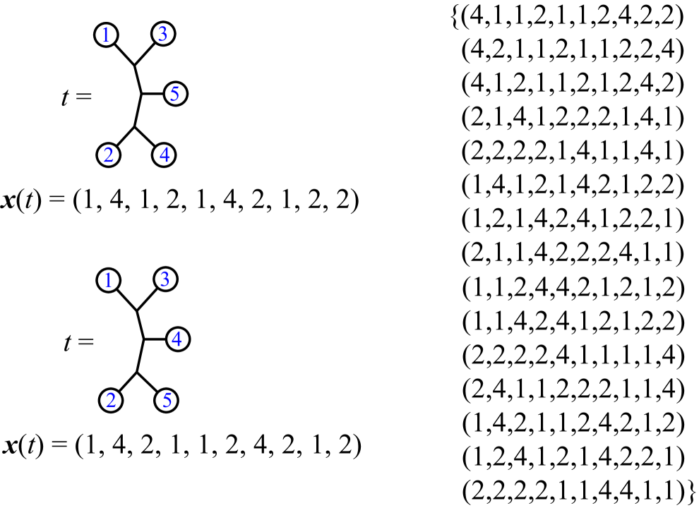
This negative fact of course raises the question of how to characterize and describe the facets of $\mathcal{P}_{n}$. We would eventually like a complete description, both combinatorially and geometrically. On the combinatorial side we would like to know which sets of vertices are those of a facet, and what other polytopes and constructions of polytopes (products, sums, pyramids, polars) those facets are equivalent to. On the geometrical side we would like to know how to quickly find the list of facet inequalities that describe $\mathcal{P}_{n}$. In Figure 3 we show the data for $n=5.$

Figure 3. Two sample vertex trees of $\mathcal{P}_{5}$ with their respective coordinates shown beneath, followed by all 15 vertex points calculated for n=5, and the $f$-vector for $\mathcal{P}_{5}$ (which gives the number of faces in each dimension starting with 0) as found by polymake [GJ00].

4. Facets from intersecting cherries.

The first type of facet of $\mathcal{P}_{5}$ that we found is associated to any pair of elements of $S=[5],$ along with a third element chosen after the pair. Thus there are ${5\choose 2}(3)=30$ of these facets. Each of these facets has its set of vertices as follows:

Theorem 4.1.

For each pair of cherries with leaves $\{a,b\}$ and $\{b,c\},$ where the pair $a,c$ and the element of intersection $b$ are three distinct elements from $S=[5],$ there is a facet of $\mathcal{P}_{5}$ whose six vertices correspond to trees that have one of the two cherries.

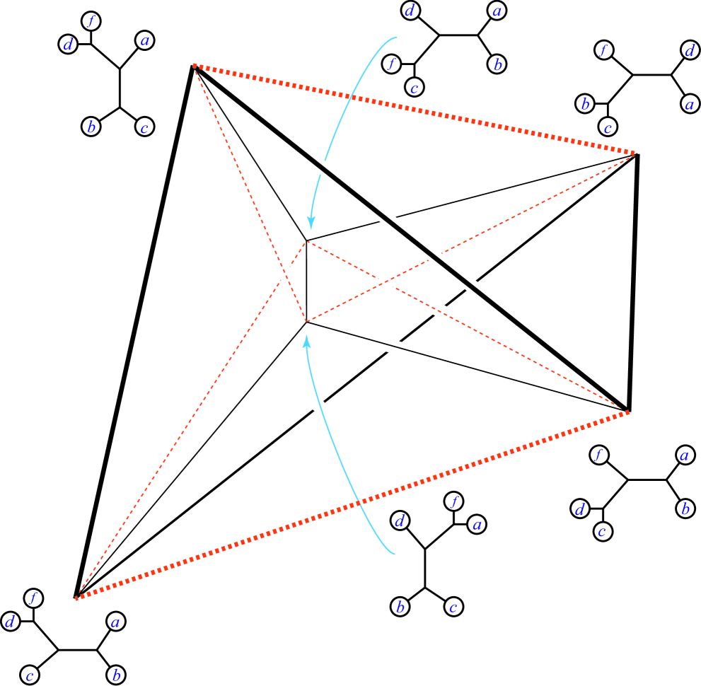
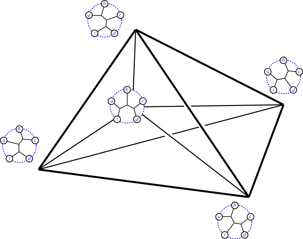
Figure 4 shows the geometry of an intersecting-cherry facet of $\mathcal{P}_{5}$.

Figure 4. A generic facet of $\mathcal{P}_{5}$ with each vertex labeled by a tree which contains one of two intersecting cherries: $\{a,b\}$ and $\{b,c\}$. The dashed edges outline the clade-faces (triangles) associated with those two cherries.

Proof.

There are six total vertices since given one of the pair of cherries there are 3 trees which have that cherry, since there are 3 elements to choose from to make the lone leaf. To show that these six vertices are the vertices of a face we need to find a linear inequality satisfied by all the vertices of $\mathcal{P}_{5}$ which becomes an equality only for the specified six vertices. Then to show that the face is a facet we need to show that its dimension is one less than the dimension of the entire polytope $\mathcal{P}_{5}$. First we show that the trees which have either a cherry with leaves $\{a,b\}$ or with leaves $\{b,c\}$ have associated points obeying:

$$x_{ab}+x_{bc}-x_{ac}=4.$$

This equation holds for our trees since if $\{a,b\}$ is the cherry then $x_{ab}=4$ and $x_{ac}=x_{bc}.$ Likewise if $\{b,c\}$ is the cherry then $x_{bc}=4$ and $x_{ac}=x_{ab}.$

Now we need to show that for any vertex that has neither of our pair of cherries, then that vertex satisfies:

$$x_{ab}+x_{bc}-x_{ac}<4.$$

This inequality holds since having neither cherry with leaves $\{a,b\}$ nor with leaves $\{b,c\}$ implies that $x_{ab}\leq 2$ and $x_{bc}\leq 2$, while we know that $x_{ac}\geq 1$.

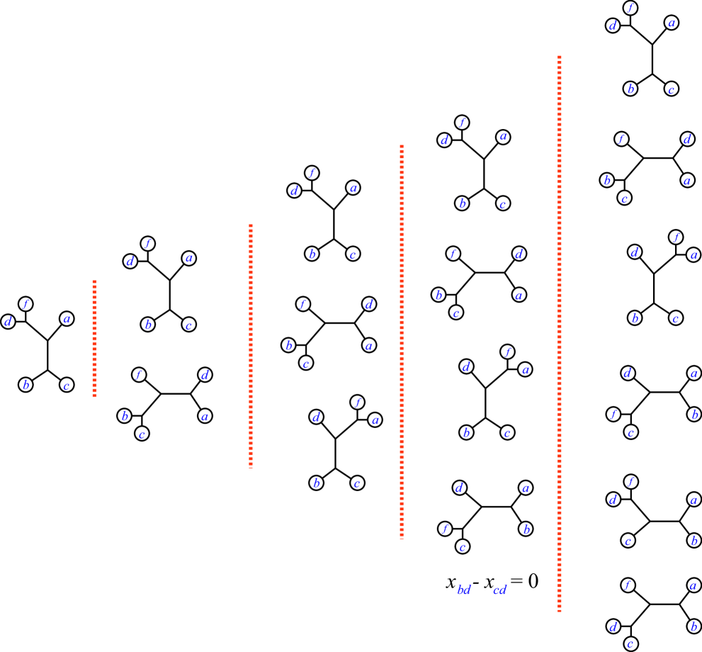
To see that our face is a 4-dimensional facet, we show that it contains a flag of subfaces (sequence of faces each contained in its successor) which is of length 5. We can proceed starting with any vertex and edge, since when $n=4$ any pair of vertices have an edge between them. Our flag chosen for the purposes of this proof is shown in Figure 5, left to right with the vertex and edge first. We choose any vertex, but then choose an edge which connects that vertex with another that shares with the first one of our special cherries, say $\{b,c\}.$

Next, the dimension 2 subface in our flag is formed by adding the third vertex that also contains the cherry $\{b,c\}.$ These three vertices form a clade face–the clade is the cherry.

The dimension 3 subface is found by adding a fourth vertex whose tree has both cherries $\{a,b\}$ and $\{c,f\}$. Together these four make a face: all four points obey the equation $x_{bd}-x_{cd}=0.$ The last two remaining trees in the facet are forced to obey $x_{bd}-x_{cd}<0.$

Figure 5. Left to right these columns show the sets of trees in faces that form a flag of a facet of $\mathcal{P}_{5}$ based on two intersecting cherries.

∎

Consider an $n\times n$ matrix as a vector with $n^{2}$ components. Taking the convex hull of the $n!$ permutation matrices gives a polytope known as $B_{n}$, or $B(n)$, the Birkhoff polytope, or assignment polytope, of order $n$. This polytope has dimension $(n-1)^{2}$, and appears in many situations, as seen in [BS96]. Here it appears again:

Theorem 4.2.

The intersecting-cherry facets of $\mathcal{P}_{5}$ are combinatorially equivalent to the Birkhoff polytope of dimension 4.

Proof.

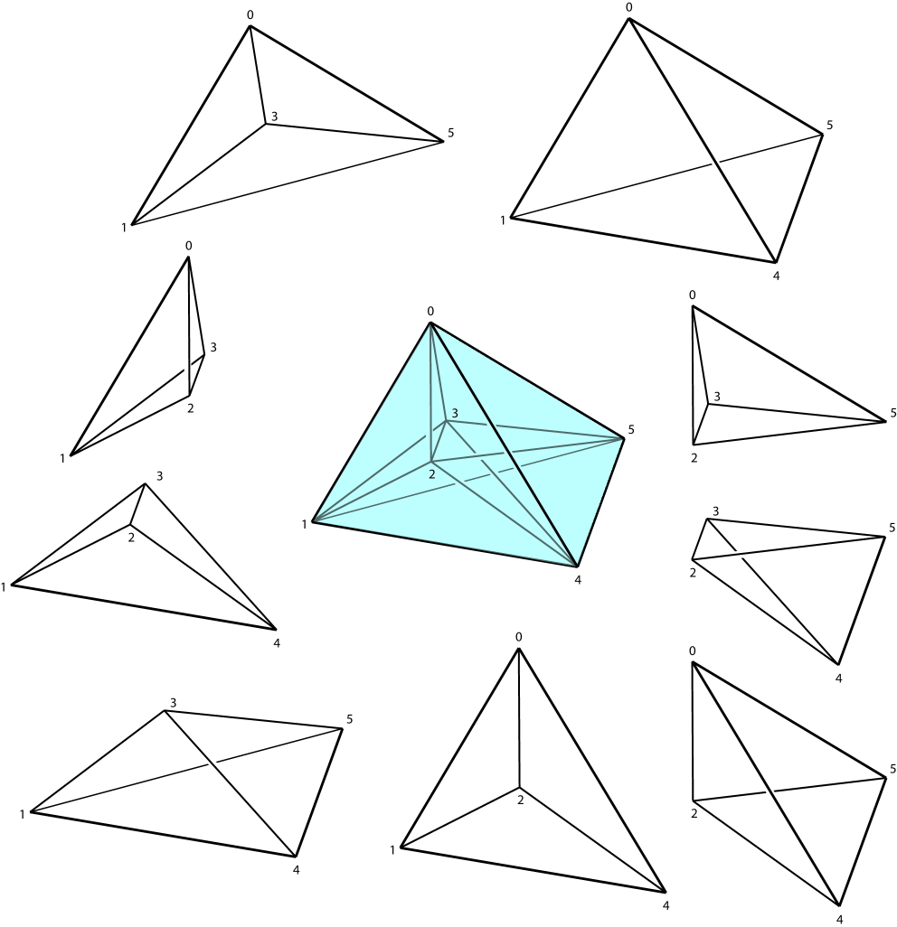
This fact was first verified by polymake for a specific intersecting-cherry facet, where the isomorphism of vertices can be seen as preserving vertex-facet incidence. Since all the intersecting-cherry facets are combinatorially equivalent by a common permutation of the coordinates, checking one is sufficient for checking all. To see the isomorphism compare the two Schlegel diagrams: from Figure 4 and from Figure 9.

∎

We leave open for future study the question of how one might determine the general isomorphism between an intersecting-cherry facet and the 4d-Birkhoff polytope. It would also be quite interesting to see if the relationship extends to higher dimensions. For now we only say the following for the general case of $\mathcal{P}_{n}$:

Theorem 4.3.

Each pair of intersecting cherries from $S=[n]$ corresponds to a certain facet of the polytope $\mathcal{P}_{n}$.

Proof.

The trees which have either a cherry with leaves $\{a,b\}$ or with leaves $\{b,c\}$ have associated points obeying:

$$x_{ab}+x_{bc}-x_{ac}=2^{n-3}.$$

This equation holds for our trees since if $\{a,b\}$ is the cherry then $x_{ab}=2^{n-3}$ and $x_{ac}=x_{bc}.$ Likewise if $\{b,c\}$ is the cherry then $x_{bc}=2^{n-3}$ and $x_{ac}=x_{ab}.$

For any vertex that has neither of our pair of cherries, then that vertex satisfies:

$$x_{ab}+x_{bc}-x_{ac}<2^{n-3}.$$

This inequality holds since having neither cherry with leaves $\{a,b\}$ nor with leaves $\{b,c\}$ implies that $x_{ab}\leq 2^{n-4}$ and $x_{bc}\leq 2^{n-4}$, while we know that $x_{ac}\geq 1$.

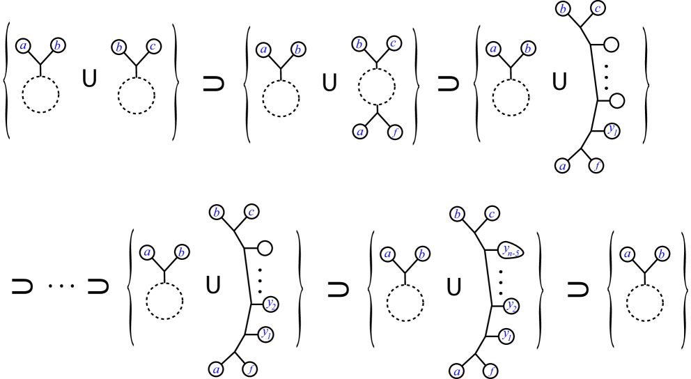
So far we have shown that the collection of trees with either cherry $\{a,b\}$ or $\{b,c\}$ forms a face $P_{abc}$ with inequality $x_{ab}+x_{bc}-x_{ac}\leq 2^{n-3}$. Next we show that the face $P_{abc}$ is in fact a facet, of dimension ${n\choose 2}-n-1.$ The strategy is to show existence of a flag of $\mathcal{P}_{n}$ beginning with $P_{abc}$ and ending with a single vertex, which has total length ${n\choose 2}-n.$ We start with a chain of sub-faces of $P_{abc}$ which has length $n-3$, including $P_{abc}$ itself. Then we show a final sub-face which has dimension ${n-1\choose 2}-(n-1)$. Thus the entire flag is of length ${n-1\choose 2}-(n-1)+1+n-3={n\choose 2}-n.$ We have illustrated this flag in Figure 6.

After $P_{abc}$ the largest face in our flag is the one whose vertices are described as each corresponding to a tree that has either the cherry $\{a,b\}$ or has both the cherry $\{b,c\}$ and the cherry $\{a,f\}$. We call this face $P_{abc,f}.$ The vertices of $P_{abc,f}$ obey the equality:

$$x_{bc}+x_{bf}-x_{ac}-x_{af}=0.$$

The trees with cherry $\{a,b\}$ have equal distances from those two leaves, while the remaining trees have coordinates $x_{bc}=x_{af}$ and $x_{bf}=x_{ac}$. Trees that have cherry $\{b,c\}$ but not cherry $\{a,f\}$ obey the inequality:

$$x_{bc}+x_{bf}-x_{ac}-x_{af}>0.$$

This is true since the tree cannot have the cherry $\{a,c\}$ either, so $x_{ac}+x_{af}\leq 2^{n-3}.$

Next, given an ordering $(y_{1},y_{2},\dots,y_{n-4})$ of the leaves not including $a,b,c$ or $f,$ there is a sequence of $n-5$ sub-faces called $P^{1}_{abc,f},P^{2}_{abc,f},\dots,P^{n-5}_{abc,f}.$ The face $P^{k}_{abc,f}$ has vertices described as each corresponding to a tree that has either the cherry $\{a,b\}$ or is a caterpillar that has both the cherry $\{a,f\}$, at one end, and the cherry $\{b,c\}$ at the other. Between the cherries in the caterpillar are the leaves $y_{1},\dots,y_{k}$ in that order beginning closest to the cherry $\{a,f\}$. The remaining leaves $y_{j}$ for $j>k$ fill in the caterpillar in any order; note that there are $n-5$ such collections since the last leaf is determined when we reach $P^{n-5}_{abc,f}.$ See Figure 6.

The vertices of $P^{k}_{abc,f}$ obey the linear equality:

$$(2^{n-3}-1)x_{ay_{k}}-(2^{n-3}-1)x_{by_{k}}+(2^{n-3-k}-2^{k})x_{ab}=(2^{n-3-k}-2^{k})2^{n-3},$$

or, more conveniently,

$$(2^{n-3}-1)(x_{ay_{k}}-x_{by_{k}})=(2^{n-3}-x_{ab})(2^{n-3-k}-2^{k}).$$

The equality is clear for trees that have the cherry $\{a,b\}$, since it becomes $0=0$. For caterpillar trees of the face $P^{k}_{abc,f}$ we have $x_{ab}=1$ and $x_{ay_{k}}-x_{by_{k}}=2^{n-3-k}-2^{k}.$

We need to show that for trees in $P_{abc,f}$ that are not in $P^{1}_{abc,f}$ we have the inequality:

$$(2^{n-3}-1)(x_{ay_{1}}-x_{by_{1}})<(2^{n-3}-x_{ab})(2^{n-3-1}-2^{1}).$$

There are two cases:

Case 1) If the tree is a caterpillar, with leaf $y_{1}$ more than two nodes from leaf $a$, then the inequality follows from $x_{ab}=1$ and $x_{ay_{1}}-x_{by_{1}}<2^{n-4}-2.$

Case 2) If the tree is not a caterpillar, we show the inequality by induction on the number $n$ of leaves. We check the base case $n=6,$ where the inequality becomes $0<(2^{3}-2)(2^{2}-2).$

Assuming the inequality for $m<n$, then in the case for $n$ leaves we choose a cherry and replace it with a single leaf. There are two subcases of Case 2.

Subcase (i): If leaf $y_{1}$ was in the chosen cherry then we call the replacement leaf $y_{1}$ instead, and by induction we have the inequality:

$$(2^{n-1-3}-1)(x_{ay_{1}}-x_{by_{1}})<(2^{n-1-3}-x_{ab}/2)(2^{n-1-4}-2).$$

where the values for the coordinates mentioned are the same as in the $n$-leaved tree before replacement.

Multiplying by 2, we get:

$(2^{n-3}-2)(x_{ay_{1}}-x_{by_{1}})<2(2^{n-1-3}-x_{ab}/2)(2^{n-5}-2)$

$=(2^{n-3}-x_{ab})(2^{n-5}-2).$

Expanding on the left and then adding to both sides gives:

$(2^{n-3}-1)(x_{ay_{1}}-x_{by_{1}})<(2^{n-3}-x_{ab})(2^{n-5}-2)+x_{ay_{1}}-x_{by_{1}}$

Expanding on the right via $2^{n-5}=2^{n-4}-2^{n-5},$ we get:

$(2^{n-3}-1)(x_{ay_{1}}-x_{by_{1}})<(2^{n-3}-x_{ab})(2^{n-4}-2)-2^{n-5}(2^{n-3}-x_{ab})+x_{ay_{1}}-x_{by_{1}}$

$=(2^{n-3}-x_{ab})(2^{n-4}-2)-(2^{n-4})^{2}+2^{n-4}x_{ab}/2)+x_{ay_{1}}-x_{by_{1}}$

Using the facts that, for our non-caterpillar tree, we know $x_{ay_{1}}-x_{by_{1}}\leq 2^{n-4}-2$ and $x_{ab}\leq 2^{n-4}$, we get:

$(2^{n-3}-1)(x_{ay_{1}}-x_{by_{1}})<(2^{n-3}-x_{ab})(2^{n-4}-2)-(\frac{1}{2}(2^{n-4})^{2}-2^{n-4}+2).$

The last term is a polynomial in $2^{n-4}$ whose minimum is $3/2$ when $n=4.$ Thus it can be dropped to achieve the desired inequality.

Subcase (ii) If leaf $y_{1}$ is not in the chosen cherry then by induction we have the inequality:

$$(2^{n-1-3}-1)(x_{ay_{1}}/2-x_{by_{1}}/2)<(2^{n-1-3}-x_{ab}/2)(2^{n-1-4}-2).$$

where the values for the coordinates mentioned are the same as in the $n$-leaved tree before replacement.

Multiplying by 4, we get:

$(2^{n-3}-2)(x_{ay_{1}}-x_{by_{1}})<(2^{n-3}-x_{ab})(2^{n-4}-4)$

Expanding on the left and then adding to both sides gives:

$(2^{n-3}-1)(x_{ay_{1}}-x_{by_{1}})<(2^{n-3}-x_{ab})(2^{n-4}-2)-2(2^{n-3}-x_{ab})+x_{ay_{1}}-x_{by_{1}}$

Using the facts that, for our non-caterpillar tree, we know $x_{ay_{1}}-x_{by_{1}}\leq 2^{n-4}-2$ and $x_{ab}\leq 2^{n-4}$, we get:

$(2^{n-3}-1)(x_{ay_{1}}-x_{by_{1}})<(2^{n-3}-x_{ab})(2^{n-4}-2)-(2^{n-2}-2^{n-3}-2^{n-4}+2)$

$=(2^{n-3}-x_{ab})(2^{n-4}-2)-(4(2^{n-4})-2(2^{n-4})-2^{n-4}+2)$

$=(2^{n-3}-x_{ab})(2^{n-4}-2)-(2^{n-4}+2).$

Since the last term is greater than 2, it can be dropped to achieve the desired inequality.

Next we need to check that for trees in $P^{k}_{abc,f}$ that are not in $P^{k+1}_{abc,f}$ we have the inequality:

$$(2^{n-3}-1)(x_{ay_{k}}-x_{by_{k}})<(2^{n-3}-x_{ab})(2^{n-3-k}-2^{k}).$$

This inequality is straightforward, since $x_{ab}=1$ and since the leaf $y_{k}$ is forced to be closer to leaf $b$ and further from leaf $a$, if it is not in the $k^{th}$ position.

Figure 6. Each set is the collection of trees (vertices of $\mathcal{P}_{n}$) that have any placement of the remaining labels from $S$ into the blank leaves shown. The containment of sets also shows the flag of our facet $P_{abc}$. The containment is $P_{abc}\supset P_{abc,f}\supset P^{1}_{abc,f}\supset P^{2}_{abc,f}\supset\dots\supset P^{n-5}_{abc,f}\supset P_{ab}.$

∎

The facet inequalities we describe in the above proof are equivalent to the triangular inequalities of Proposition 3 in [CLPSG12]. This connection does raise the question of whether other inequalities in that paper can lead to facets of the BME polytope.

Note that the dimension of a general face corresponding to an intersecting pair of cherries is greater than the dimension of the clade-face for the clade that is one of those cherries. We conjecture based on initial experiments (verified by polymake for $n$=6) that in fact the dimension is ${n\choose 2}-n-1,$ implying that these intersecting-cherry faces are indeed facets. We also leave for the future the investigation of other sorts of intersecting sets of clades: we conjecture that two or three or more clades, of various sizes and tree geometry, intersecting in various ways, will lead to further faces and facets of $\mathcal{P}_{n}$.

5. Facets from free cyclic orderings.

A free circular permutation (or free cyclic ordering, or necklace) of the elements of $S$ is only distinguished by which elements are adjacent. It is an arrangement of the elements of $S$ around a circle, which may be rotated or flipped. We are interested in the binary trees on $S$ which are coplanar with a certain free cyclic ordering on $S.$ That is, having drawn one of the two planar versions of the cyclic ordering, we can then draw the tree in the same plane, as in Figure 7. The number of trees coplanar with the free cyclic ordering is found by a simple counting argument for $n=5:$ there are 5 choices for the first cherry and the two for the second cherry; but then we divide by two since the order we choose the cherries in is irrelevant, giving us five total trees.

Theorem 5.1.

For each free cyclic ordering $\mathcal{N}$ on $S$ with $|S|=5$ there is a facet of $\mathcal{P}_{5}$ that is equivalent to a 4-simplex, whose five vertices correspond to trees that are coplanar with the free cyclic ordering.

Proof.

The trees which are coplanar with $\mathcal{N}=(a,b,c,d,f)$ satisfy $x_{ab}+x_{bc}+x_{cd}+x_{df}+x_{fa}=13.$ That is because two cherries are represented by those components, and the remaining components are assigned values 2, 2 and 1 respectively. All other trees in $\mathcal{P}_{5}$, not coplanar with $\mathcal{N}$, obey $x_{ab}+x_{bc}+x_{cd}+x_{df}+x_{fa}<13.$ That is because at most one cherry can be among those components, and the rest of the components then can at most be assigned the value 2. Thus the components add up to at most 12.

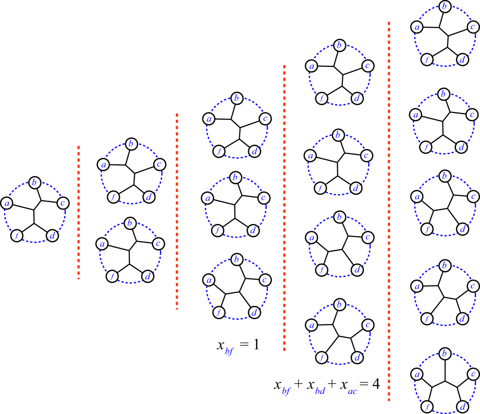
Thus our five trees constitute the vertices of a face of $\mathcal{P}_{5}$. We show that this is a facet, with dimension equal to 4, by establishing within it a flag of length 5. We can proceed starting with any vertex and edge, since any pair of vertices have an edge between them. Our flag chosen for the purposes of this proof is shown in Figure 8, left to right with the vertex and edge first. The set of three vertices makes a triangular face of the facet since they obey the equality $x_{bf}=1$ while the other two vertices have $x_{bf}>1.$ The set of four vertices make a 3-simplex since they all obey the equality $x_{bf}+x_{bd}+x_{ac}=4,$ while the final vertex has $x_{bf}+x_{bd}+x_{ac}>4.$

Figure 7. A generic facet of $\mathcal{P}_{5}$ based on a free cyclic ordering $(a,b,c,d,f)$.

Figure 8. Left to right these columns show the sets of trees in faces that form a flag of a facet of $\mathcal{P}_{5}$ based on a free cyclic ordering $(a,b,c,d,f)$.

∎

The number of free cyclic orderings on 5 objects is $4!/2=12.$ Via polymake we see that there are exactly 12 facets of $\mathcal{P}_{5}$ that have 5 vertices. Thus we have accounted for all of these facets with free cyclic orderings.

6. Facets from Caterpillars.

The third type of facet for $\mathcal{P}_{5}$ corresponds to a choice of two elements of $S.$ These are placed as leaves on a tree that are as far apart as possible: in this case a distance of 3 internal nodes on a binary caterpillar. Thus there are six ways to place the remaining three elements of $S$ as the other three leaves, and the caterpillar facet has 6 vertices.

Theorem 6.1.

Each pair of elements ${a,b}$ from $S$ with $|S|=5$ determines a facet of $\mathcal{P}_{5}$ whose vertices are trees that have $a$ and $b$ as leaves of distinct cherries.

Proof.

The result follows from the general Theorem 6.3 which establishes the fact for all dimensions. Specifically, each tree that has the elements $a$ and $b$ separated by 3 internal nodes has corresponding vector that obeys $x_{ab}=1.$ All other trees, which do not have this property, obey $x_{ab}>1.$ The flag of length 5 which establishes that the face in question is indeed a facet is described inductively in the proof of Theorem 6.3. ∎

The number of these facets in $\mathcal{P}_{5}$ is ${5\choose 2}=10.$ Note that now we have described $30+12+10=52$ facets of $\mathcal{P}_{5},$ the total number predicted by polymake. The three classes of facets do not intersect for $n=5$: that is, a caterpillar facet cannot be an intersecting cherry facet (nor vice-versa), since the collection of caterpillar trees is determined by choosing two leaves to be as far apart as possible, while the intersecting cherry trees allow any two leaves to be closer than the maximum distance.

Theorem 6.2.

The caterpillar facets of $\mathcal{P}_{5}$ are combinatorially equivalent to the Birkhoff polytope of dimension 4.

Proof.

This fact was first verified by polymake, where the isomorphism of vertices may be seen as preserving vertex-facet incidence. Since all the caterpillar facets are combinatorially equivalent by a common permutation of the coordinates, checking one is sufficient for checking all. We illustrate the isomorphism by showing the two Schlegel diagrams in Figure 9. ∎

Figure 9. On the top is the Birkhoff polytope $B(3)$ with vertices labeled by the permutation matrices. On the bottom is a facet of $\mathcal{P}_{5}$ with each vertex labeled by the tree corresponding to the permutation matrix in the corresponding position.

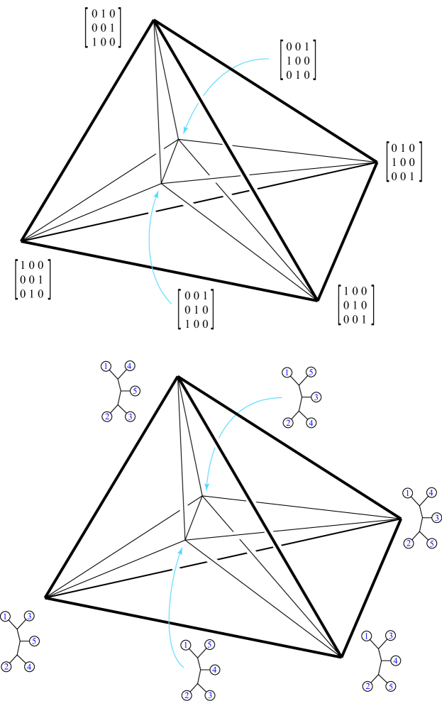
The generalization of this caterpillar facet for any size set $S$ has vertices any collection of trees with leaves $S$ that are all binary caterpillars, with a pair of chosen species as the two which must reside as far apart as possible–as leaves of the only two distinct cherries. These faces are indeed facets of $\mathcal{P}_{n},$ each with $(n-2)!$ vertices. In general they are not equivalent to the Birkhoff polytope $B(n-2)$, since for $n>5$ the facets of $\mathcal{P}_{n}$ have a dimension ${n\choose 2}-n-1$ which is greater than $(n-3)^{2}$ (the dimension of $B(n-2).$) However an interesting projection is suggested by the 4-dimensional case in Figure 9, where a permutation matrix corresponding to permutation $\sigma$ is mapped to the tree with leaves 3,4, and 5 in the order $\sigma(3),\sigma(4),\sigma(5)$. We leave as an open question, for instance, whether this map in the general case gives rise to a cellular projection to the Birkhoff polytope from facets of the balanced minimal evolution polytope.

Theorem 6.3.

Consider the set of binary caterpillar trees on $n$ leaves $S$ with a given pair from the set $S$ as maximally separated leaves. The vertices of $\mathcal{P}_{n}$ calculated from these caterpillar trees are the vertices of a facet of $\mathcal{P}_{n}$.

Note that the number of these facets in $\mathcal{P}_{n}$ is ${n\choose 2}$ for $n>4.$ For $n=4$ there are half that many, the three edges of the triangle in Figure 2, since having chosen two elements of $S$ to be placed in the distinct cherries we automatically determine the other two elements which will also be placed in distinct cherries: in the notation of the proof that follows we have for instance that $P^{4}_{12}=P^{4}_{34}.$

Proof.

of Theorem 6.3 For the purposes of this proof we choose the set $S=[n]$ and without loss of generality we let the two fixed leaves with maximal distance $n-2$ between them be the leaves labeled 1 and 2. We’ll continue by choosing leaves in counting order: this will be without loss of generality since any other selection of leaves is covered by choosing an appropriate ordering.

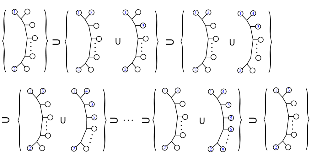
Thus the caterpillar trees with fixed leaves 1 and 2 obey $x_{12}=1$, and all other points in $\mathcal{P}_{n}$ obey $x_{12}>1.$ We call this face $P^{n}_{12}.$ Next we use induction on $n$, the number of leaves, to show that the face $P^{n}_{12}$ is in fact a facet, of dimension ${n\choose 2}-n-1.$ The strategy is to show existence of a flag of $\mathcal{P}_{n}$ beginning with $P^{n}_{12}$ and ending with a single vertex, which has total length ${n\choose 2}-n.$ We start with a chain of sub-faces of $P^{n}_{12}$ which has length $n-2$, including $P^{n}_{12}$ itself. Then we show a final sub-face which has the same dimension as $P^{n-1}_{12}$, thus inductively of dimension ${n-1\choose 2}-(n-1)-1.$ Thus the entire flag is of length ${n-1\choose 2}-(n-1)+n-2={n\choose 2}-n.$

The base case of our induction is $n=4.$ See Figure 2 where each edge of the triangle is a facet of this type. Specifically, the edge $P^{4}_{12}$ is at the bottom of the triangle.

After $P^{n}_{12}$ the largest face in our flag is the one whose vertices are described as vertices of $P^{n}_{12}$ whose caterpillar tree is one of two types, as seen in Figure 10. The tree has a third fixed leaf, say the leaf labeled 3, either in the same cherry as the leaf 1; or as the leaf nearest that cherry but not in it. We call this face $P^{n}_{12,3}$, and note that it contains $2((n-3)!)$ vertices. To see that it is indeed a face, we show that its vertices obey the equation

$$x_{13}+2^{n-4}\left(\sum_{i=4}^{n}(x_{1i}-x_{3i})\right)=2^{n-3}.$$

…and that all other vertices in $P^{n}_{12}$ obey the inequality:

$$x_{13}+2^{n-4}\left(\sum_{i=4}^{n}(x_{1i}-x_{3i})\right)>2^{n-3}.$$

First, the vertices of $P^{n}_{12}$ whose caterpillar tree has the leaf labeled 3 in the same cherry as the leaf 1: for these the difference $x_{1i}-x_{3i}=0$ for each $i,$ while $x_{13}=2^{n-3}$. For the vertices that have leaf 3 as the leaf nearest the cherry containing leaf 1, but not in it: $x_{13}=2^{n-4}$ and the sum of differences telescopes and simplifies to equal $2^{n-n}=1.$ The equality holds since $2(2^{n-4})=2^{n-3}.$

Any other leaf of $P^{n}_{12}$ not in $P^{n}_{12,3}$ has leaf 3 even further from the cherry containing leaf 1. Now the sum of differences will telescope and simplify to become $1+2+\dots+2^{j}$ where $j$ is the number of leaves further (than 1) from the cherry that leaf 3 is found. Since the latter sum is larger than 2, the left side of our inequality is greater than $2^{n-3}.$

Next we describe a sequence of $n-4$ nested faces (of steadily smaller dimension) labeled $P^{n}_{12,34},P^{n}_{12,345},\dots,P^{n}_{12,345\dots k}$ for $k=4\dots n-1.$ The vertices of $P^{n}_{12,34}$ (the first in this series, with largest dimension) are vertices of $P^{n}_{12,3}$ which either have leaf 3 in the cherry with leaf 1, or have leaf 4 in the cherry with leaf 1. After that, for $k>4$ the vertices of $P^{n}_{12,34\dots k}$ are vertices of $P^{n}_{12,34\dots(k-1)}$ with either leaf 3 in the cherry with leaf 1 or leaf 4 in the cherry with leaf 1 and leaves $5\dots k$ in that order immediately on the other side of leaf 3. See Figure 10.

First we show that the vertices of $P^{n}_{12,345\dots k}$ obey the equality:

$$2^{n-k}x_{13}+2^{n-4}\left(\sum_{i=4}^{k}(x_{1i}-x_{3i})\right)=2^{n-3}2^{n-k}.$$

Consider the vertices of $P^{n}_{12,345\dots k}$ whose caterpillar tree has the leaf labeled 3 in the same cherry as the leaf 1: for these the difference $x_{1i}-x_{3i}=0$ for each $i,$ while $x_{13}=2^{n-3}$. For the vertices that have leaf 3 as the leaf nearest the cherry containing leaf 1, but not in it: $x_{13}=2^{n-4}$ and the sum of differences telescopes and simplifies to equal $2^{n-k}.$ The equality holds since $2(2^{n-4})=2^{n-3}.$

To check for the needed inequalities we begin with $k=4.$ We show that the vertices of $P^{n}_{12,3}$ which are not in $P^{n}_{12,34}$ obey the inequality:

$$2^{n-k}x_{13}+2^{n-4}\left(\sum_{i=4}^{k}(x_{1i}-x_{3i})\right)<2^{n-3}2^{n-k}.$$

For $k=4$, and since these trees have leaf 3 as the leaf nearest the cherry containing leaf 1, but not in it, and leaf 4 also not in that cherry, this inequality becomes:

$$2^{n-4}2^{n-4}+2^{n-4}\left(x_{14}-x_{34}\right)<2^{n-3}2^{n-4}.$$

This inequality holds since $x_{14}-x_{34}<0,$ and so $2^{n-4}+(x_{14}-x_{34})<2^{n-4}<2^{n-3},$ which leads to the desired inequality.

Now, for $k>4,$ we need to show that the vertices of $P^{n}_{12,3\dots k-1}$ which are not in $P^{n}_{12,3\dots k}$ obey the inequality:

$$2^{n-k}x_{13}+2^{n-4}\left(\sum_{i=4}^{k}(x_{1i}-x_{3i})\right)>2^{n-3}2^{n-k}.$$

Since these trees have leaf 3 as the leaf nearest the cherry containing leaves 1 and 4, this inequality becomes:

$$2^{n-k}2^{n-4}+2^{n-4}\left(\sum_{i=4}^{k}(x_{1i}-x_{3i})\right)>2^{n-3}2^{n-k}.$$

Since leaf $k$ is at a position farther from leaf 1 than if the tree was in $P^{n}_{12,3\dots k},$ then the sum of differences telescopes and simplifies to $2^{n-k+1}-2^{x}$ where $x<n-k.$ Thus $x-(n-k)<0$ and it is clear that $1+2-2^{x-(n-k)}>2.$ Therefore:

$$2^{n-k}2^{n-4}+2^{n-4}2^{n-k}(2-2^{x-(n-k)})>2^{n-3}2^{n-k},$$

which is the simplified inequality we needed to show.

Finally we reach the subface called $P^{n}_{123},$ which consists of the vertices of $P^{n}_{12,345\dots n-1}$ which have leaf 3 in the same cherry as leaf 1. That of course means they are only of the first type. They constitute a subface, since they obey the additional equality $x_{13}=2^{n-3},$ while the other vertex of $P^{n}_{12,345\dots n-1}$ obeys $x_{13}=2^{n-4}<2^{n-3}.$ We check that this face $P^{n}_{123}$ projects to $P^{n-1}_{12},$ which as discussed above will give us the correct number of remaining faces of our flag, by induction. The linear projection is described by its action on the ${n\choose 2}$ coordinates, yielding ${n-1\choose 2}$ new ones; thus it is given by an ${n-1\choose 2}\times{n\choose 2}$ matrix $A$, which has rows and columns labeled by the respective coordinates in lexicographic order.

First each coordinate involving leaf 3 (so $x_{i3}$ or $x_{3i}$) is discarded. That means the columns of $A$ corresponding to these coordinates are made up of zeroes. Second, the coordinates that involve leaf 1 (so $x_{i1}$ or $x_{1i}$) are multiplied by 1, but sent to the new coordinates with the same label if $i=2,$ or to the coordinates $x_{(i-1)1}$ or $x_{1(i-1)}$ respectively if $i\geq 4.$ Thus the columns of $A$ corresponding to these coordinates have a single entry of 1 in the row corresponding to the new coordinate. Finally the coordinates $x_{ij}$ involving neither leaf 1 nor leaf 3 are multiplied by $1/2$ and sent to the new coordinate $x_{i^{\prime}j^{\prime}}$ where $i^{\prime}=i-1$ for $i>2$ and $i^{\prime}=i$ for $i=2$; and likewise for $j^{\prime}.$ Thus the columns of $A$ corresponding to these coordinates have a single entry of $1/2$ in the row corresponding to the new coordinate. For instance here is the matrix $A$ for $n=5$; it takes the two sample vectors listed in Figure 3 (the two vertices of the lowest edge in Figure 9) to the two vectors labeling the lower edge of the triangle in Figure 2.

$$A=\left[\begin{array}[]{cccccccccc}1&0&0&0&0&0&0&0&0&0\\ 0&0&1&0&0&0&0&0&0&0\\ 0&0&0&1&0&0&0&0&0&0\\ 0&0&0&0&0&1/2&0&0&0&0\\ 0&0&0&0&0&0&1/2&0&0&0\\ 0&0&0&0&0&0&0&0&0&1/2\\ \end{array}\right]$$

We claim that the image of $P^{n}_{123}$ under $A$ is the polytope $P^{n-1}_{1,2}.$ This follows from the fact that the projection $A$ induces a 1-1 and onto mapping between the vertices of the two polytopes. Since there are $(n-3)!$ vertices of each polytope, the surjective property of the mapping implies that it is a bijection. We can easily describe the preimage of a vertex in $P^{n-1}_{12}:$ take its caterpillar tree, attach a new branch as close to leaf 1 as possible, and give it leaf 3. Then add 1 to increment each of the other leaves except for leaf 2. The resulting new tree has the coordinates required. The coordinates involving leaf 3 will be discarded, so their value can be ignored. The leaves in our new tree are all now one node further away from leaf 1, but using the new total number of leaves $n$ this difference is canceled. The coordinates involving neither leaf 1 nor leaf 3 are the same except for the factor of 2.

Figure 10. Each set is the collection of trees (vertices of $\mathcal{P}_{n}$) that have any placement of the remaining labels from $S=[n]$ into the blank leaves shown. The containment of sets also shows the flag of our facet $P^{n}_{12}$. The containment is $P^{n}_{12}\supset P^{n}_{12,3}\supset P^{n}_{12,34}\supset P^{n}_{12,345}\supset\dots\supset P^{n}_{12,345\dots n-1}\supset P^{n}_{123}.$ Note that the next to last set also has leaf $n$ fixed since there is only one place for it, and the last set (bottom right) is the set of vertices of $\mathcal{P}_{n}$ which label a face that projects to the facet $P^{n-1}_{12}.$

∎

Figure 11. Here we show the facets of the 4-dimensional Birkhoff polytope. Each of the nine tetrahedra has its vertices labeled to show where it fits in the central Schlegel diagram.

7. Acknowledgements

We would like to thank the referees, whose suggestions helped to improve the readability of this paper. The first author would like to thank the organizers and participants in the Working group for geometric approaches to phylogenetic tree reconstructions, at the NSF/CBMS Conference on Mathematical Phylogeny held at Winthrop University in June-July 2014. Especially helpful were conversations with Ruriko Yoshida, Terrell Hodge and Matt Macauley. The first author would also like to thank the American Mathematical Society and the Mathematical Sciences Program of the National Security Agency for supporting this research through grant H98230-14-0121. The first author’s specific position on the NSA is published in [For14]. Suffice it to say here that he appreciates NSA funding for open research and education, but encourages reformers of the NSA who are working to ensure that protections of civil liberties keep pace with intelligence capabilities.

References

- [BS96] Louis J. Billera and A. Sarangarajan. All - polytopes are traveling salesman polytopes. Combinatorica, 16(2):175–188, 1996.
- [CLPSG12] Daniele Catanzaro, Martine Labbé, Raffaele Pesenti, and Juan-José Salazar-González. The balanced minimum evolution problem. INFORMS J. Comput., 24(2):276–294, 2012.
- [Day87] William H. E. Day. Computational complexity of inferring phylogenies from dissimilarity matrices. Bull. Math. Biol., 49(4):461–467, 1987.
- [DG02] Richard Desper and Olivier Gascuel. Fast and accurate phylogeny reconstruction algorithms based on the minimum-evolution principle. J. Comp. Biol., 9(5):687–705, 2002.
- [EHPY08] K. Eickmeyer, P. Huggins, L. Pachter, and R. Yoshida. On the optimality of the neighbor-joining algorithm. Alg. Mol. Biol., 3, 2008.
- [FJ12] Samuel Fiorini and Gwenaël Joret. Approximating the balanced minimum evolution problem. Oper. Res. Lett., 40(1):31–35, 2012.
- [For14] S. Forcey. Dear NSA: Long-term security depends on freedom. Notices of the AMS, 61(1), 2014.
- [GJ00] Ewgenij Gawrilow and Michael Joswig. polymake: a framework for analyzing convex polytopes. In Gil Kalai and Günter M. Ziegler, editors, Polytopes — Combinatorics and Computation, pages 43–74. Birkhäuser, 2000.
- [GS06] O. Gascuel and M. Steel. Neighbor-joining revealed. Mol. Biol. and Evol., 23:1997–2000, 2006.
- [HHY11] David C. Haws, Terrell L. Hodge, and Ruriko Yoshida. Optimality of the neighbor joining algorithm and faces of the balanced minimum evolution polytope. Bull. Math. Biol., 73(11):2627–2648, 2011.
- [Hug08] P. Huggins. Polytopes in computational biology. Ph.D. Dissertation, U.C. Berkeley, 2008.
- [Pau00] Yves Pauplin. Direct calculation of a tree length using a distance matrix. J. of Mol. Evol., 51(1):41–47, 2000.
- [SN87] N. Saitou and M. Nei. The neighbor joining method: a new method for reconstructing phylogenetic trees. Mol. Biol. and Evol., 4:406–425, 1987.