Globally Optimal Cell Tracking using Integer Programming

Abstract

We propose a novel approach to automatically tracking cell populations in time-lapse images. To account for cell occlusions and overlaps, we introduce a robust method that generates an over-complete set of competing detection hypotheses. We then perform detection and tracking simultaneously on these hypotheses by solving to optimality an integer program with only one type of flow variables. This eliminates the need for heuristics to handle missed detections due to occlusions and complex morphology. We demonstrate the effectiveness of our approach on a range of challenging sequences consisting of clumped cells and show that it outperforms state-of-the-art techniques.

1 Introduction

	Source Images	Segmentation	CT [36]	JST [35]	KTH [25]	OURS	Ground Truth
t=76
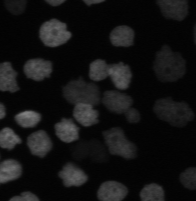
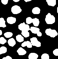
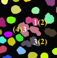
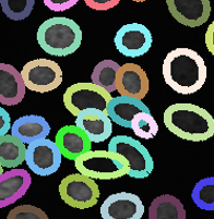
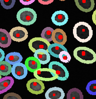
t=77
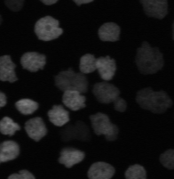
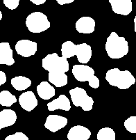
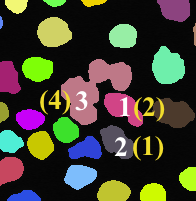
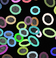
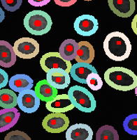
t=78

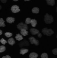
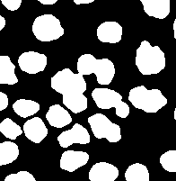
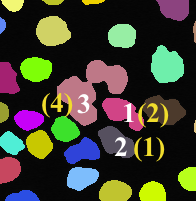
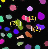
Figure 1: Three images from a typical sequence; the original segmentations produced by a pixel-based classifier; the results of [36](CT), [35](JST), [25](KTH), and our method (OURS); the manually annotated tracking ground truth in red dots and the optimal ellipse-tracks obtained using this ground truth. The track identities are encoded in colors. Our approach correctly tracks the cells in spite of long-term segmentation failures, and produce results that are very similar to the ground truth. In the CT, JST and KTH columns, the white-colored numbers indicate the tracker-inferred numbers of cells that are contained by the segments beneath them, and the yellow-colored numbers show the ground truth. Best viewed in color.

Detecting and tracking cells over time is key to understanding cellular processes including division (mitosis), migration, and death (apoptosis). Modern microscopes produce vast image streams making manual tracking tedious and impractical. High-throughput automated systems are therefore increasingly in demand and several cell tracking competitions have recently been organized to attract Computer Vision researchers’ interest and speed up progress [28, 38]. These competitions have shown that state-of-the-art methods are still error-prone due to occlusions, imaging noise, and complex cell morphology.

Cell tracking is an instance of the more generic multi-target tracking problem with the additional difficulties that cells, unlike for example pedestrians, can either divide or wither away and disappear in mid-sequence. In its generic form, the problem is often formulated as a two-step process that involves first detecting potential objects in individual frames and then linking these detections into complete trajectories. This approach is attractive because spurious detections, such as false positives due to imaging noise and artifacts, can be eliminated by imposing temporal consistency across many frames, which is more difficult to do in recursive approaches.

Many of the most successful algorithms to both people [12, 3, 41, 40] and cell tracking [24, 20, 36] follow this two-step approach by first running an object detector on each frame independently and building a graph whose nodes are the detections and edges connect pairs of them. They then find a subgraph that represents object trajectories by considering the whole graph at once. However, to handle missed detections, these methods often rely on heuristic procedures that offer no guarantee of optimality. This is of particular concern for cell tracking because detections are often unreliable due to the complex morphology of cell populations. For example, in Fig. 1, groups of cells that appear clumped together in some frames can only be told apart when considering the sequence as a whole.

The approach proposed in [35] addresses this issue by introducing a factor graph for joint cell segmentation and tracking. Inference is then achieved by solving a relatively complex integer program that involves several types of variables and constraints. The algorithm starts from a watershed-based oversegmentation that is sensitive to inaccuracies in pixel probability estimates. It is therefore subject to errors when the cells are clumped together and hard to distinguish from each other.

In this paper, we formulate joint detection and tracking in terms of constrained Bayesian inference. This lets us cast the problem as an integer program expressed in terms of a single type of flow variables. To explicitly account for the often ambiguous output of cell detectors, we devised a robust ellipse-fitting algorithm to generate multiple and potentially conflicting initial hypotheses from the output of a foreground-background segmentation algorithm, as depicted by Fig. 2. We then model critical cell events, such as migration and division, using flow variables and resolve the conflicts by solving the resulting integer program, which is conceptually much simpler than those of earlier approaches [20, 36, 16, 35]. It also features fewer variables and constraints, which implies better scaling properties.

Although network flow formulation has been used in this context before, existing approaches [31, 32] focus on cell tracking in consecutive image pairs, while our approach aggregates image evidences from the whole sequence and conducts global optimization over all potential cell locations at all time frames. Furthermore, we handle competing hypotheses within the same optimization framework instead of having to decide at detection time.

We show that this improves trajectories and yields superior detection performance on various datasets compared to the recent approaches of [36, 1, 26, 35], which includes the technique that performed best on the above-mentioned cell-tracking challenges [28, 38].

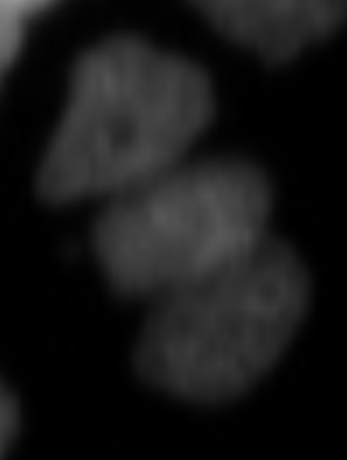
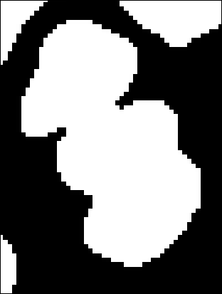
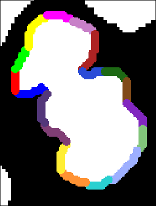
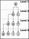
(a) Image	(b) Segmentation	(c) Contourlets	(d) Hierarchy
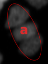
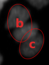
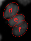
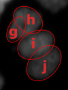
(e) Level 1	(f) Level 2	(g) Level 3	(h) Level 4

Figure 2: Hierarchy of detection hypotheses. (a) An image region containing three HeLa cells clumped together. (b) Applying a pixel classifier results in under-segmentation, in which the three cells appear as a single connected component. (c) Automatically extracted contourlets for this component. Each one is overlaid in a different color. They are used to fit ellipses using a hierarchical agglomerative clustering algorithm. (d) The resulting hierarchy of 10 hypotheses. We show only the first four levels for simplicity. (e-h) Individual levels with one, two, three and four hypotheses.

2 Related Work

Current tracking approaches can be divided into Tracking by Model Evolution and Tracking by Detection [28]. We briefly discuss state-of-the-art representatives of these two classes below and refer the interested reader to the much more complete recent surveys [29, 28].

2.1 Tracking by Model Evolution

Most algorithms in this class simultaneously track and detect objects greedily from frame to frame. This means extrapolating results obtained in earlier frames to process the current one, which can be done at a low computational cost and is therefore fast in practice. Such methods have attracted attention both in the cell tracking field [9, 8, 7, 27] as well as in the more general object tracking one [43, 18, 30, 42, 11]. Common techniques in the cell tracking category involve evolving appearance or geometry models from one frame to the next, typically done using active contours [9, 8, 7, 27] or Gaussian Mixture Models [1]. Though these methods are attractive and mathematically sound, performance suffers from the fact that they only consider a restricted temporal context and therefore cannot guarantee consistency over a whole sequence.

This limitation has been addressed by more global active contour methods [23, 33] that consider the whole spatio-temporal domain to segment the cells and recover parts of their trajectories. Although this provides improved robustness at the cost of increased computational burden, these approaches do not provide global optimality either.

2.2 Tracking by Detection

Approaches in this class have proved successful at both people [12, 5, 3, 41, 40, 15] and cell tracking [24, 20, 36].

They involve first detecting the target objects in individual frames and then linking these detections to produce full trajectories. This is typically computationally more expensive than Tracking by Model Evolution. However, it also tends to be more robust because trajectories are computed by minimizing a global objective function that enforces consistency of appearance, disappearance, and division over time. This can be seen in the benchmark of [28] in which these methods tended to dominate.

One way to perform tracking-by-detection is to reason in the full spatio-temporal grid formed by stacking up all possible spatial locations over time [4, 2, 34, 14, 22]. This can be done optimally in polynomial time for non-dividing objects such as pedestrians and has made this approach competitive despite the large size of the graphs involved. However, for dividing objects, the resulting optimization problem is NP-Hard, which is why this dense spatio-temporal approach has not been explored for cell tracking.

Instead, practical tracking-by-detection algorithms for cells rely on a small number of strong detections that can be later linked into complete trajectories. Recent efforts have focused on solving two main challenges specific to cell-tracking, which we discuss below.

Division and disappearance. Cells can divide or die and disappear. While rule-based approaches have been used to handle this, most recent ones formulate tracking as a global IP [20, 36]. This makes it possible to use priors for cell migration, division and disappearance between adjacent frames. One notable exception is the method of [25] that relies on the Viterbi algorithm to sequentially add trajectories to a cell lineage tree. Motion, division, and disappearance are encoded through a scoring function that quantifies how well the lineage tree explains the data. This algorithm scored highest in one of the benchmarks [28] and we will use it as one of our baselines in Section 4.

Clumped cells. There is no guarantee that individual cells will be detected as separate entities in any given frame because two or more cells can clump together, producing under-segmentation errors. Many heuristics have been proposed to solve this problem. One is to assume that clumped cells are unlikely to happen for a specific modality or that they do not pose a problem for the tracker [24, 20, 25]. While this is appropriate in some cases, it is clearly invalid for certain modalities such as the one shown in Fig. 1. Other heuristics involve splitting segmentations using the Radon and watershed transforms [9, 28]. Unfortunately, they are still relatively prone to over- and under-segmentation that complicate the tracking task. The approach of [21] generates oversegmentation by fitting ellipses on Hessian Images. However, this approach focuses on developing embryo and relies on strong assumptions, such as assuming that the number of cells do not decrease from time $t$ to $t+1$.

An ingenious approach is that of [36], which first finds trajectories by treating segmentations in each frame as clumps of one or more cells, with the exact number being initially unknown, and then uses a factor graph to resolve this ambiguity. However, since the final linking is decoupled from the cell cluster tracking, the cell count inaccuracies may propagate to the final trajectories. To overcome this problem, [35] introduces a set of hypotheses, generated by over-segmenting the image into superpixels and subsequently merging them to create competing explanations. Similarly, [17] generates the hypotheses using component trees and graph cut. However, neither method uses spatially overlapping hypotheses and may result in irrecoverable segmentation errors. By contrast, our approach naturally handles such cases, as depicted by Fig. 2. Furthermore, as we will discuss in Section 3.2, our formulation provides a more compact integer program with much less constraints and variables.

3 Method

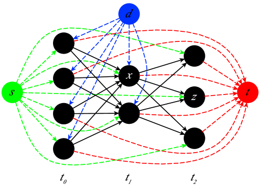
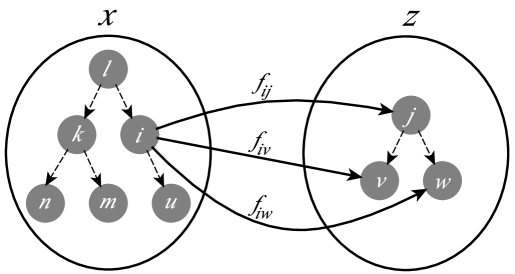
(a)	(b)

Figure 3: Spatio-temporal graph of hypotheses for 3 consecutive time frames. (a) Each black circle is a hypervertex corresponding to a connected component of the segmentation and is connected to neighboring ones at the next time step. The special vertices $s$ (source, in green), $t$ (sink, in red) and $d$ (division, in blue) allow respectively for cell appearance, disappearance and division. (b) Each hypervertex, such as $x$ and $z$, contains a hierarchical set of hypotheses (vertices) such as those depicted by Fig. 2. These hypotheses are shown as gray circles and connected to nearby ones in the following frame via directed edges. We only show three of these edges to avoid clutter. On each hypervertex, we define an exclusion set for each leaf vertex. For example, we define three exclusion sets on $x$: $S_{n}=\{l,k,n\}$, $S_{m}=\{l,k,m\}$ and $S_{u}=\{l,i,u\}$. We allow the tracker to select at most one vertex within each one. Best viewed in color.

Our approach involves building a spatio-temporal graph of conflicting detection hypotheses and then finding the globally optimal trajectories in it. More specifically, we first produce a binary image of the underlying cell populations using a classifier trained on a few hand-annotated segmentations. For each connected component, we produce multiple hypotheses by hierarchically fitting a varying number of ellipses to it. This results in a directed graph, such as the one depicted by Fig. 3. Its nodes are individual ellipses and its edges connect nearby ones in consecutive frames. Full trajectories can then be obtained by solving an integer program with a small number of constraints that exclude incompatible hypotheses and enforce consistency while allowing for cell-division, migration and death.

In the following, we first describe our approach to segmenting cell images and building hypotheses graphs from them. We then formulate the simultaneous detection and tracking problem on these graphs as a constrained network flow problem, and discuss how we compute the various energy terms of its objective function.

3.1 Building Hierarchy Graphs

Our algorithm, like those of [24, 20, 36], starts by segmenting cells using local image features. To this end, we first train the binary random forest pixel classifier of [37] for each evaluation dataset on a few partially annotated images. We use four different types of low-level features: pixel intensities, gradient and hessian values, and difference of Gaussians, all of which are computed by first Gaussian smoothing the input image with a range of sigma values.

Applying the resulting classifier to the full image sequences results in segmentations which often contain groups of clumped cells, such as the ones shown in Fig. 1. Therefore, each connected component of the segmentation potentially contains an a priori unknown number of cells.

We produce a hierarchy of conflicting detection hypotheses for each such component by fitting a varying number of ellipses to its contours. More specifically, we first identify all the contour points that are local maxima of curvature magnitude. This is done iteratively by selecting the maximum curvature points and suppressing their local neighborhoods. We then break the contour into short segments at these points, which yields a number of contourlets as shown in Fig. 2(c). We cluster them in a hierarchical agglomerative fashion and fit ellipses to each resulting cluster using the non-iterative least squares approach of [6]. In all our experiments, we set the size of the suppression neighborhood to seven pixels because this is the minimum number of points required to reliably fit an ellipse using this approach.

Let $C$ denote the set of all contourlet clusters for a connected component. Given a pair of clusters $C_{i}\in C$ and $C_{j}\in C$, we define their distance to be

$$\bigg{[}\sum_{C_{l}\in\{C_{i}\cup C_{j}\}}{h(C_{l},e)}+\sum_{C_{l}\in C\setminus\{C_{i}\cup C_{j}\}}{g(C_{l},e)}\bigg{]}c(e)\sqrt{\frac{1}{1+ec^{2}(e)}}\ ,$$ (1)

where $e$ is the ellipse obtained by fitting to the points of $C_{i}\cup C_{j}$, and $c(e)$ and $ec(e)$ are its circumference and eccentricity respectively. $h(C_{l},e)$ denotes the Hausdorff distance between the points of $C_{l}$ and the ellipse $e$. The function $g(C_{l},e)$ is defined in a similar way but without considering the points of $C_{l}$ that are outside $e$.

The first term in the product captures image evidence along the contours of the entire connected component while the last two ones act as a shape regularizer to prevent implausible ellipse geometries from appearing in the solution. We use this distance measure to compute an ellipse hierarchy, such as the one of Fig. 2, for every connected component in the temporal sequence.

Given these over-complete hierarchies, we then build a graph, whose vertices are the ellipses and the edges link pairs of them that belong to two spatially close connected components in consecutive frames. The resulting graph has a hierarchical dimension that allows for finding the globally optimal cell detections and trajectories in a single shot.

3.2 Network Flow Formalism

The procedure described above yields a directed graph $G^{\prime}=(V^{\prime},E^{\prime})$, which we then augment with three distinguished vertices; namely the source $s$, the sink $t$ and the division $d$ as depicted by Fig. 3. We connect these three vertices to every other vertex in $G^{\prime}$ to allow accounting for cell appearance, disappearance and division in mid-sequence.

Let $G=(V,E)$ be the resulting graph obtained after the augmentation. We define a binary flow variable $f_{ij}$ for each edge $e_{ij}\in E$ to indicate the presence of any one of the following cellular events:

• Cell migration from vertex $i$ to vertex $j$,

• Appearance at vertex $j$, if $i=s$,

• Division at vertex $j$, if $i=d$,

• Disappearance at vertex $i$, if $j=t$.

Let $\mathbf{f}$ be the set of all $f_{ij}$ flow variables and $\mathbf{F}=\{F_{ij}\}$ be the set of all corresponding hidden variables. Given an image sequence $\mathbf{I}\!=(\mathbf{I}^{1},\dots,\mathbf{I}^{T})$ with $T$ temporal frames and the corresponding graph $G$, we look for the optimal trajectories $\mathbf{f}^{*}$ in $G$ as the solution of

$$\mathbf{f}^{*} = \underset{\mathbf{f}\in{\cal F}}{\operatorname{argmax}}\,P(\mathbf{F}=\mathbf{f}\mid\,\mathbf{I})$$ (2)

$$\approx \underset{\mathbf{f}\in{\cal F}}{\operatorname{argmax}}\prod_{e_{ij}\in E}P(F_{ij}=f_{ij}\mid\mathbf{I}^{t(i)},\mathbf{I}^{t(j)})$$ (4)

$$= \underset{\mathbf{f}\in{\cal F}}{\operatorname{argmax}}\prod_{e_{ij}\in E}P(F_{ij}=1\mid\mathbf{I}^{t(i)},\mathbf{I}^{t(j)})^{f_{ij}}\times$$

$$\hskip 49.0ptP(F_{ij}=0\mid\mathbf{I}^{t(i)},\mathbf{I}^{t(j)})^{(1-f_{ij})}$$

$$= \underset{\mathbf{f}\in{\cal F}}{\operatorname{argmax}}\sum_{e_{ij}\in E}\log\left(\frac{P(F_{ij}=1\mid\mathbf{I}^{t(i)},\mathbf{I}^{t(j)})}{P(F_{ij}=0\mid\mathbf{I}^{t(i)},\mathbf{I}^{t(j)})}\right)f_{ij}\,$$ (6)

$$= \underset{\mathbf{f}\in{\cal F}}{\operatorname{argmax}}\sum_{e_{ij}\in E^{\prime}}\log\left(\frac{\rho_{ij}}{1-\rho_{ij}}\right)f_{ij}+\sum_{j\in V}\log\left(\frac{\rho_{a}}{1-\rho_{a}}\right)f_{sj}$$

$$+\sum_{i\in V}\log\left(\frac{\rho_{d}}{1-\rho_{d}}\right)f_{it}+\sum_{j\in V}\log\left(\frac{\rho_{j}}{1-\rho_{j}}\right)f_{dj}\ ,$$

where $\mathbf{I}^{t(i)}$ is the temporal frame containing vertex $i$, and ${\cal F}$ denotes the set of all feasible cell trajectories, which satisfy linear constraints. In Eq. 4, we assume that the flow variables $F_{ij}$ are conditionally independent given the evidence from consecutive frame pairs. Eqs. 4 and 6 are obtained by using the fact that the flow variables are binary and by taking the logarithm of the product. Finally, in Eq. 6, we split the sum into four parts corresponding to the four events mentioned above.

The appearance and disappearance probabilities, $\rho_{a}$ and $\rho_{d}$, are computed simply by finding the relative frequency of these events in the ground truth cell lineages of the training sequences. On the other hand, the migration and the division probabilities, $\rho_{ij}$ and $\rho_{j}$, are obtained using a classification approach as described in the next section.

We define three sets of linear constraints to model cell behavior and exclude conflicting detection hypotheses from the solution, which we describe in the following.

Conservation of Flow:

We require the sum of the flows incoming to a vertex to be equal to the sum of the outgoing flows. This allows for all the four cellular events while incurring their respective costs given in Eq. 6.

$$\sum_{e_{ij}\in E^{\prime}}f_{ij}+f_{sj}+f_{dj}=\sum_{e_{jk}\in E^{\prime}}f_{jk}+f_{jt}\ ,\hskip 14.22636pt\forall j\in V^{\prime}\ .$$ (7)

Prerequisite for Division:

We allow division to take place at a vertex $j\in V^{\prime}$ only if there is a cell at that location. We write this as

$$\sum_{e_{ij}\in E^{\prime}}f_{ij}+f_{sj}\geq f_{dj}\ ,\hskip 14.22636pt\forall j\in V^{\prime}\ .$$ (8)

Exclusion of Conflicting Hypotheses:

Given a hierarchy tree of detections, we define an exclusion set $S_{l}$ for each terminal vertex $l\in V^{\prime}$ of this tree. For instance, in the example of Fig. 2(d), the four exclusion sets are $\{a,b,d,g\}$, $\{a,b,d,h\}$, $\{a,b,e,i\}$ and $\{a,c,f,j\}$. Let $S$ be the collection of all such sets for all the connected components in the sequence. We disallow more than one vertex from each set to appear in the solution, and express this as

$$\sum_{\begin{subarray}{c}j\in S_{l},\\ e_{ij}\in E^{\prime}\end{subarray}}f_{ij}+\sum_{j\in S_{l}}f_{sj}\leq 1,\hskip 14.22636pt\forall S_{l}\in S\ .$$ (9)

We solve the resulting integer programs within an optimality tolerance of $1e^{-3}$ using the branch-and-cut algorithm implemented in the Gurobi optimization library [13].

Note that our integer program contains only a single set of variables and three sets of linear constraints, and therefore it is more compact than those of the recent approaches of [35] and [36] that are similar to ours. Formally, let $N$, $C$, and $K$ denote the total number of detections, total number of exclusion sets and average number of neighbors per detection. The total number of constraints for ours and [35] are $C+2N$ and $C+2N+2NK$; the total number of variables are $N(3+K)$ and $N(1+K+2^{(K+1)})$ respectively. The term $2^{(K+1)}$ comes from the fact that [35] includes indicator variables for higher order factors.

3.3 Cell Migration and Division Classifiers

Given two adjacent vertices $i,j\in V^{\prime}$, and their associated ellipses $e_{i}$ and $e_{j}$ in consecutive time frames, we train a classifier to estimate the likelihood that both belong to the same cell. More specifically, we use a Gradient Boosted Tree (GBT) classifier [10] to learn a function $\varphi_{\textrm{migr}}(e_{i},e_{j})\in\mathbb{R}$, based on both appearance and geometry features including the distance between the ellipses, their eccentricities and degree of overlap, hierarchical fitting errors and ray features. Once $\varphi_{\textrm{migr}}(e_{i},e_{j})$ is learned, we apply Platt scaling to compute the probability $\rho_{ij}$ that the two ellipses belong to the same cell, and plug it into Eq. 6.

Similarly, the likelihood of ellipse $e_{j}$ at time $t$ dividing into two ellipses $e_{k}$ and $e_{l}$ at $t+1$ is learned with another GBT classifier, trained on features such as the orientation and size differences among the ellipses. We present a detailed list of both the migration and division features in the Supplementary Material.

For prediction, we compute the division score for ellipse $e_{j}$ at time $t$ as

$$\varphi_{\textrm{div}}(e_{j})=\max_{\begin{subarray}{c}e_{jk}\in E^{\prime},\ e_{jl}\in E^{\prime}:\\ k\neq l\end{subarray}}\ \ \ \varphi_{\textrm{div}}(e_{j},e_{k},e_{l})\>,$$ (10)

where $\varphi_{\textrm{div}}(\cdot,\cdot,\cdot)$ is the scoring function learned by the classifier, and $(e_{k},e_{l})$ is a pair of ellipses corresponding to two potential daughter cells at time $t+1$. We obtain the division probability $\rho_{j}$ of Eq. 6 from $\varphi_{\textrm{div}}(e_{j})$, again using Platt scaling.

4 Experiments

In this section, we first introduce the datasets and state-of-the-art methods we use as baselines for evaluation purposes. We then demonstrate that our approach significantly outperforms these baselines, especially when the cells divide or are not well separated in the initial segmentations. Our software can be downloaded from an URL to be specified in the final version of the paper and the corresponding tracking videos are available as supplementary material.

4.1 Test Sequences

We used 10 image sequences from three datasets of the cell tracking challenge [38]. They involve multiple cells that migrate, appear, disappear, and divide. Difficulties arise from low contrast to the background, complex cell morphology, and significant mutual overlap. We used the leave-one-out training and testing scheme within each dataset to train the classifiers of Section 3.3 and to learn the appearance and disappearance probabilities of Eq. 6.

• HeLa Dataset: It comprises two 92-frame sequences from the MitoCheck consortium. Cell divisions are frequent, which produces a dense population with severe occlusions.

• SIM Dataset: It comprises six 50- to 100-frame sequences. They simulate migrating and dividing nuclei on a flat surface.

• GOWT Dataset: It comprises two 92-frame sequences of mouse stem cells. Their appearance varies widely and some have low contrast against a noisy background.

			Division			Detection			Migration			MOTA	TRA	Time
			Rec	Pre.	F-M.	Rec.	Pre.	F-M.	Rec.	Pre.	F-M.
HeLa-1		GMM	0.56	0.43	0.48	N/A	N/A	N/A	0.92	0.98	0.95	0.82	N/A	44
		KTH	0.65	0.72	0.68	N/A	N/A	N/A	0.95	0.99	0.97	0.91	0.98	70
		CT	0.74	0.79	0.77	0.56	0.89	0.69	0.94	0.99	0.97	N/A	N/A	74.85
		JST	0.79	0.55	0.65	N/A	N/A	N/A	0.86	0.92	0.89	0.73	0.80	128.16
		OURS	0.92	0.79	0.85	0.96	0.83	0.89	0.97	0.99	0.98	0.94	0.98	88.25
HeLa-2		GMM	0.40	0.18	0.24	N/A	N/A	N/A	0.95	0.98	0.97	0.43	N/A	74
		KTH	0.65	0.72	0.68	N/A	N/A	N/A	0.94	0.99	0.97	0.90	0.97	336
		CT	0.76	0.81	0.78	0.73	0.63	0.67	0.94	0.99	0.96	N/A	N/A	79.33
		JST	0.69	0.44	0.54	N/A	N/A	N/A	0.91	0.98	0.94	0.82	0.85	88.79
		OURS	0.86	0.83	0.84	0.86	0.78	0.82	0.96	0.99	0.97	0.90	0.97	232.31
GOWT-2		GMM	0.0	0.0	0.0	N/A	N/A	N/A	0.16	0.79	0.26	0.02	N/A	37
		KTH	0.0	N/A	0.0	N/A	N/A	N/A	0.94	1.0	0.97	0.94	0.91	16
		CT	1.0	0.17	0.29	1.0	0.02	0.03	0.95	1.0	0.97	N/A	N/A	0.81
		JST	1.0	0.02	0.04	N/A	N/A	N/A	0.93	0.98	0.95	0.85	0.95	3.87
		OURS	1.0	1.0	1.0	1.0	1.0	1.0	0.95	1.0	0.98	0.96	0.95	0.22
SIM-4		GMM	0.25	0.33	0.29	N/A	N/A	N/A	0.91	0.94	0.92	0.81	N/A	23
		KTH	0.75	0.75	0.75	N/A	N/A	N/A	0.97	0.99	0.98	0.96	0.98	5
		CT	0.75	0.60	0.67	0.75	0.68	0.72	0.86	0.97	0.92	N/A	N/A	1.69
		JST	0.75	0.38	0.50	N/A	N/A	N/A	0.96	0.96	0.96	0.84	0.96	4.33
		OURS	1.0	0.80	0.89	1.0	0.79	0.88	0.98	1.0	0.99	0.96	1.0	1.85

Table 1: Comparison of our algorithm against state-of-the-art cell trackers in terms of tracking accuracy and running time. It yields a significant improvement on the division and detection accuracies and performs either on par or slightly better on the migration, MOTA and TRA scores.

4.2 Baselines

We compared our algorithm (OURS) against the following four state-of-the-art methods

• Gaussian Mixture-based Tracker (GMM) [1]: We ran the Gaussian Mixture Models approach of [1], originally designed to track cell nuclei, whose code is publicly available. We manually tuned its parameters to the ones that yield the best results on each sequence.

• KTH Cell Tracker (KTH) [25]: The code is publicly available and has been reported to perform best in the Cell Tracking Challenge [38, 28]. We used the parameter settings optimized for each dataset and provided in the software package.

• Conservation Tracking (CT) [36]: We ran Ilastik V1.1.3 [39] that implements the method of [36]. We used the default parameters provided with the tool to handle appearance, disappearance, division and transition weights. The CT algorithm, like ours, requires initial segmentations such as the ones shown in the second column of Fig.1. We used the same segmentations for both algorithms. We trained the division and the segment count classifiers separately for each dataset on manually labeled cells.

• Joint Segmentation and Tracking (JST) [35]: We ran the code of [35] that is publicly available. The model comprises several parameters for oversegmentation and tracking, which we tuned to achieve the best possible result on each sequence.

It is worth noting that, in contrast to all the above state-of-the-art trackers, our tracker does not require any user-defined parameters.

To demonstrate the importance of individual components of our approach, we also ran simplified versions of OURS with various features turned off:

• Classifier Only (OURS-CL): We threshold the output of our migration and division classifiers at a probability of 0.5 and return the resulting ellipse detections.

• Best Hierarchy Only (OURS-BH): For each ellipse hierarchy tree, we only keep the level that yields the minimum fitting error, which we define in the Supplementary Material. We then run our IP optimization on the resulting graphs, which are smaller than the ones we normally use.

• Linear Programming Relaxation (OURS-LP): We relax the integrality constraint on the variables and solve the optimization problem of Eq. 6 using linear programming. We then round the resulting fractional values to the nearest integer to obtain the final solution.

• No Conflict Set Constraint (OURS-NC): We remove the conflict set constraints of Eq. 9 and solve the resulting integer program as before.

• Fixed Division Cost (OURS-FD): We set the division probability to a constant $p_{d}$, which we compute by finding the relative frequency of the division event in the training sequences.

4.3 Evaluation Metrics

We use precision, recall and the F-Measure, defined as the harmonic mean of precision and recall, to quantify the algorithms’ ability to detect cell division, detection, and migration events. We also use two global metrics, multiple object tracking accuracy (MOTA) [19] and tracking precision (TRA) [38], to evaluate the overall tracking performance.

We follow the same evaluation methodology as in [36], which uses the connected components of the initial segmentations to compute the division, detection, and migration accuracies. We consider a cell migration event to be successfully detected if both connected components of the cell at $t$ and $t+1$ are correctly identified. Similarly, we consider a division event to be successfully detected if it occurs at the correct time instant with the connected components of the parent and both daughter cells correctly determined. Finally, a detection event is said to be successfully identified if an algorithm infers the right number of cells within a connected component.

Unlike the above measures, MOTA and TRA are defined on individual cell tracks rather than connected components that potentially contain multiple clumped cells. They therefore provide a global picture of tracking performance. The main difference between TRA and MOTA is, TRA defines different penalties for different types of errors, while MOTA treat all errors equally.

		Division			Detection			Migration			MOTA
		Rec	Pre.	F-M.	Rec.	Pre.	F-M.	Rec.	Pre.	F-M.
HeLa-1	OURS-CL	0.95	0.06	0.11	N/A	N/A	N/A	0.98	0.47	0.64	N/A
	OURS-NC	0.48	0.14	0.22	0.0	0.0	0.0	0.96	0.93	0.94	-0.61
	OURS-FD	0.78	0.81	0.80	0.96	0.85	0.90	0.97	0.99	0.98	0.93
	OURS-BH	0.88	0.73	0.80	0.81	0.87	0.84	0.97	0.99	0.98	0.94
	OURS-LP	0.92	0.80	0.86	0.95	0.81	0.87	0.97	0.99	0.98	0.93
	OURS	0.92	0.79	0.85	0.96	0.83	0.89	0.97	0.99	0.98	0.94
HeLa-2	OURS-CL	0.91	0.10	0.18	N/A	N/A	N/A	0.92	0.60	0.72	N/A
	OURS-NC	0.73	0.31	0.43	0.06	0.02	0.02	0.95	0.96	0.95	0.35
	OURS-FD	0.77	0.82	0.80	0.84	0.78	0.81	0.96	0.98	0.97	0.90
	OURS-BH	0.84	0.77	0.81	0.78	0.77	0.77	0.95	0.99	0.97	0.90
	OURS-LP	0.85	0.83	0.84	0.84	0.78	0.81	0.95	0.99	0.97	0.90
	OURS	0.86	0.83	0.84	0.86	0.78	0.82	0.96	0.99	0.97	0.90
GOWT-2	OURS-CL	0.0	0.0	0.0	N/A	N/A	N/A	0.94	0.94	0.94	N/A
	OURS-NC	1.0	0.20	0.33	1.0	0.02	0.03	0.96	1.0	0.98	0.93
	OURS-FD	1.0	0.25	0.40	1.0	1.0	1.0	0.96	1.0	0.98	0.96
	OURS-BH	0.0	N/A	0.0	1.0	1.0	1.0	0.91	1.0	0.95	0.91
	OURS-LP	1.0	0.50	0.67	1.0	0.50	0.67	0.96	1.0	0.98	0.96
	OURS	1.0	1.0	1.0	1.0	1.0	1.0	0.96	1.0	0.98	0.96
SIM-4	OURS-CL	0.75	0.27	0.40	N/A	N/A	N/A	0.92	0.56	0.70	N/A
	OURS-NC	0.75	0.21	0.33	0.37	0.19	0.25	0.97	0.98	0.98	0.58
	OURS-FD	0.75	0.75	0.75	0.98	0.78	0.87	0.98	1.0	0.99	0.95
	OURS-BH	1.0	0.80	0.89	1.0	0.78	0.87	0.98	1.0	0.99	0.96
	OURS-LP	1.0	0.80	0.89	1.0	0.79	0.88	0.98	1.0	0.99	0.96
	OURS	1.0	0.80	0.89	1.0	0.79	0.88	0.98	1.0	0.99	0.96

Table 2: Tracking results with various features turned off. OURS-CL does not impose temporal consistency and suffers from low precision. OURS-NC imposes temporal consistency in the optimization but allows multiple conflicting hypotheses to appear in the solution, which yields a low precision. OURS-FD eliminates competing hypotheses but uses a fixed cost for the division event. OURS-BH performs non-maxima suppression on the hierarchical dimension and hence suffers from mis-detection errors. OURS-LP yields fractional flows and the rounding stage eliminates some cell tracks, which leads to a slight drop in performance. With all its features turned on, OURS achieves the best overall performance.

4.4 Comparing against the Baselines

We ran our algorithm and the baselines discussed above on all the test sequences introduced in Section 4.1. Table 1 summarizes the results for a representative subset and the remainder can be found in the supplementary material.

Some numbers are missing because the publicly-available implementation of CT [36] we use does not provide the identities of individual cells in under-segmentation cases. We therefore cannot extract the complete tracks required to compute the MOTA and TRA scores. For our method and that of CT, we computed the detection scores by using the same segmentations obtained from the pixel classification approach of Section 3.1. By contrast, GMM [1], KTH [25] and JST [35] trackers take only raw images as input and do not accept external segmentations to be used. Therefore, we cannot compute their accuracy for the detection events. Finally, in some cases, GMM generates non-consecutive cell tracks, which is not accepted by the TRA evaluation software.

Table 1 shows that our tracker consistently yields a significant improvement on the division and detection events. Even on the migration events for which the baselines already perform very well, we do slightly better. However, because the division and detection events are rare compared to migrations, the significant improvements on these two events only have a small impact on MOTA and TRA.

The comparatively poor performance of GMM can be partially ascribed to the fact that it relies on a simple hand-designed appearance and geometry model to detect individual cells. KTH relies on a richer appearance model that improves performance but requires tuning more parameters for each sequence. CT employs several cell-event classifiers and solves the tracking problem using integer programming, resulting in an overall higher division accuracy. Finally, the performance of JST is negatively impacted by the fact that it depends on a watershed-based oversegmentation that is sensitive to inaccuracies in pixel probability estimates. By contrast, our ellipse-fitting approach to generating competing hypotheses is robust to the ambiguous image evidence. Given the same initial segmentation as CT, our method achieves the best overall performance, thanks to the simultaneous detection and tracking.

Our tracker runs relatively fast even though we use a large number of variables. We show in Tab. 1 the running time of all trackers given the detections. In the SIM-4 case, the number of flow variables is around 1.1 million but the integer programming optimization takes only 2 seconds. In the HeLa-2 case, the number of variables is around 8 million and the optimization takes about 232 seconds.

4.5 Evaluating Individual Components

To produce the results summarized by Table 1, we used our full approach as described in Section 3. In Table 2, we show what happens when we turn off some of its components to gauge their respective impacts.

OURS-CL relies on local classifier scores and does not impose temporal consistency. That is why, it produces a large number of spurious cell tracks. OURS-NC addresses this by imposing temporal consistency but it allows multiple conflicting hypotheses to be active simultaneously. Therefore, it still suffers from spurious detections, which leads to low precision. OURS-FD disallows conflicting detections but relies on a fixed division probability, which is why it gives low division performance. OURS-BH uses division classifier costs but collapses the hierarchical dimension of our graphs and results in mis-detections. Finally, OURS-LP removes the integrality constraints on the flow variables. This gives a similar performance to OURS on most of the sequences suggesting that the integrality constraints are seldom helpful. However, in the case of HeLa-2, where division events are frequent, we observed that around 3% of the non-zero flow variables are fractional, which explains the 2% drop in recall compared to OURS.

5 Conclusion

We have introduced a novel approach to automatically detecting and tracking cell populations in time-lapse images. Unlike earlier approaches that rely either on heuristics to handle mis-detections due to occlusions, or on complex integer programs with large sets of variables and constraints, our approach yields a simple integer program for simultaneously detecting and tracking cells over time. Furthermore, we present a robust algorithm for generating over-complete detection hypotheses based on fitting ellipses hierarchically. This results in more accurate trajectories and improved detection of mitosis events.

Furthermore, the formalism is very generic. In future work, we plan to apply it to people tracking and, in particular, modeling how groups can form and unform.

References

- [1] F. Amat, W. Lemon, D. Mossing, K. McDole, Y. Wan, K. Branson, E. Myers, and P. Keller. Fast, Accurate Reconstruction of Cell Lineages from Large-Scale Fluorescence Microscopy Data. Nat. Methods, 2014.
- [2] A. Andriyenko and K. Schindler. Globally Optimal Multi-Target Tracking on a Hexagonal Lattice. In ECCV, pages 466–479, 2010.
- [3] A. Andriyenko, K. Schindler, and S. Roth. Discrete-Continuous Optimization for Multi-Target Tracking. In CVPR, 2012.
- [4] J. Berclaz, F. Fleuret, E. Türetken, and P. Fua. Multiple Object Tracking Using K-Shortest Paths Optimization. PAMI, 33(11):1806–1819, September 2011.
- [5] R. Collins and P. Carr. Hybrid Stochastic / Deterministic Optimization for Tracking Sports Players and Pedestrians. In ECCV, 2014.
- [6] D. K. Prasad and M. K. H. Leung and C. Quek. ElliFit: An Unconstrained, Non-Iterative, Least Squares-based Geometric Ellipse Fitting Method. PR, 46(5):1449–1465, 2013.
- [7] R. Delgado-gonzalo, N. Chenouard, and M. Unser. Fast Parametric Snakes for 3D Microscopy. In ISBI, pages 852–855, 2012.
- [8] A. Dufour, R. Thibeaux, E. Labruyere, N. Guillen, and J.-C. Olivo-Marin. 3D Active Meshes: Fast Discrete Deformable Models for Cell Tracking in 3D Time-Lapse Microscopy. TIP, 20(7):1925–1937, 2011.
- [9] O. Dzyubachyk, W. V. Cappellen, J. Essers, W. Niessen, and E.Meijering. Advanced Level-Set-Based Cell Tracking in Time-Lapse Fluorescence Microscopy. TMI, 2010.
- [10] J. Friedman. Stochastic Gradient Boosting. Computational Statistics & Data Analysis, 2002.
- [11] J. Gall, A. Yao, N. Razavi, L. Van Gool, and V. Lempitsky. Hough Forests for Object Detection, Tracking, and Action Recognition. PAMI, 2011.
- [12] W. Ge and R. T. Collins. Multi-Target Data Association by Tracklets with Unsupervised Parameter Estimation. In BMVC, September 2008.
- [13] Gurobi. Gurobi Optimizer, 2012. http://www.gurobi.com/.
- [14] H. Heibel, B. Glocker, M. Groher, M. Pfister, and N. Navab. Interventional Tool Tracking Using Discrete Optimization. TMI, 32(3):544–555, 2013.
- [15] H. Jiang, S. Fels, and J. Little. A Linear Programming Approach for Multiple Object Tracking. In CVPR, 2007.
- [16] F. Jug, T. Pietzsch, D. Kainmüller, and G. Myers. Tracking by Assignment Facilitates Data Curation. In MICCAI IMIC Workshop, 2014.
- [17] F. Jug, T. Pietzsch, D. Kainmüller, J. Funke, M. Kaiser, E. van Nimwegen, C. Rother, and G. Myers. Optimal Joint Segmentation and Tracking of Escherichia Coli in the Mother Machinen. In MICCAI BAMBI Workshop, 2014.
- [18] Z. Kalal, K. Mikolajczyk, and J. Matas. Tracking-Learning-Detection. PAMI, 34(07), July 2012.
- [19] R. Kasturi, D. Goldgof, P. Soundararajan, V. Manohar, J. Garofolo, M. Boonstra, V. Korzhova, and J. Zhang. Framework for Performance Evaluation of Face, Text, and Vehicle Detection and Tracking in Video: Data, Metrics, and Protocol. PAMI, 31(2):319–336, February 2009.
- [20] B. Kausler, M. Schiegg, B. Andres, M. Lindner, U. Koethe, H. Leitte, J. Wittbrodt, L. Hufnagel, and F. Hamprecht. A Discrete Chain Graph Model for 3D+ T Cell Tracking with High Misdetection Robustness. In ECCV, pages 144–157, 2012.
- [21] A. Khan, S. Gould, and M. Salzmann. A Linear Chain Markov Model for Detection and Localization of Cells in Early Stage Embryo Developmenty. In WACV, pages 526–533, 2014.
- [22] J. Kim, A. Bartoli, T. Collins, and R. Hartley. Tracking by Detection for Interactive Image Augmentation in Laparoscopy. Biomedical Image Registration, pages 246–255, 2012.
- [23] H. Li, R. Sumner, and M. Pauly. Global Correspondence Optimization for Non-Rigid Registration of Depth Scans. In Symposium on Geometry Processing, pages 1421–1430, 2008.
- [24] K. Li, E. D. Miller, M. Chen, T. Kanade, L. E. Weiss, and P. G. Campbell. Cell Population Tracking and Lineage Construction with Spatiotemporal Context. MIA, 12(5):546–566, 2008.
- [25] K. Magnusson and J. Jalden. A Batch Algorithm Using Iterative Application of the Viterbi Algorithm to Track Cells and Construct Cell Lineages. In ISBI, 2012.
- [26] K. Magnusson, J. Jalden, P. Gilbert, and H. Blau. Global Linking of Cell Tracks Using the Viterbi Algorithm. TMI, 2014.
- [27] M. Maška, O. Daněk, S. Garasa, A. Rouzaut, A. Munoz-barrutia, and C. O. de solorzano. Segmentation and Shape Tracking of Whole Fluorescent Cells Based on the Chan-Vese Model. TMI, 32(6):995–1006, 2013.
- [28] M. Maška, V. Ulman, D. Svoboda, P. Matula, P. Matula, C. Ederra, A. Urbiola, T. España, S. Venkatesa, D. Balak, et al. A Benchmark for Comparison of Cell Tracking Algorithms. Bioinf., 30(11):1609–1617, 2014.
- [29] E. Meijering, O. Dzyubachyk, and I. Smal. Methods for Cell and Particle Tracking. Methods in Enzymology, 504(9):183–200, 2012.
- [30] S. Oron, A. Bar-hillel, and S. Avidan. Extended Lucas-Kanade Tracking. In ECCV, 2014.
- [31] D. Padfield, J. Rittscher, and B. Roysam. Coupled Minimum-Cost Flow Cell Tracking. In IPMI, 2009.
- [32] D. Padfield, J. Rittscher, and B. Roysam. Coupled Minimum-Cost Flow Cell Tracking for High-Throughput Quantitative Analysis. MIA, 15(4):650–668, 2011.
- [33] D. Padfield, J. Rittscher, N. Thomas, and B. Roysam. Spatio-Temporal Cell Cycle Phase Analysis Using Level Sets and Fast Marching Methods. MIA, 13(1):143–155, 2009.
- [34] H. Pirsiavash, D. Ramanan, and C. Fowlkes. Globally-Optimal Greedy Algorithms for Tracking a Variable Number of Objects. In CVPR, June 2011.
- [35] M. Schiegg, P. Hanslovsky, C. Haubold, U. Koethe, L. Hufnagel, and F. A. Hamprecht. Graphical Model for Joint Segmentation and Tracking of Multiple Dividing Cells. Bioinf., 2014.
- [36] M. Schiegg, P. Hanslovsky, B. Kausler, L. Hufnagel, and F. Hamprecht. Conservation Tracking. In ICCV, pages 2928–2935, December 2013.
- [37] J. Schindelin, I. Arganda-Carreras, E. Frise, V. Kaynig, M. Longair, T. Pietzsch, S. Preibisch, C. Rueden, S. Saalfeld, and B. Schmid. Fiji: an open-source platform for biological-image analysis. Nat. Methods, 9(7):676–682, 2012. Code available at http://pacific.mpi-cbg.de.
- [38] C. O. Solorzano, M. Kozubek, E. Meijering, and A. M. noz Barrutia. ISBI Cell Tracking Challenge, 2014.
- [39] C. Sommer, C. Straehle, U. Koethe, and F. Hamprecht. ilastik: Interactive Learning and Segmentation Toolkit. In ISBI, 2011.
- [40] C. Wojek, S. Walk, S. Roth, , K. Schindler, and B. Schiele. Monocular Visual Scene Understanding: Understanding Multi-Object Traffic Scenes. PAMI, 2013.
- [41] B. Yang and R. Nevatia. An Online Learned CRF Model for Multi-Target Tracking. In CVPR, 2012.
- [42] J. Zhang, S. Ma, and S. Sclaroff. MEEM: Robust Tracking via Multiple Experts Using Entropy Minimization. In ECCV, 2014.
- [43] K. Zhang, L. Zhang, Q. Liu, D. Zhang, and M.-H. Yang. Fast Tracking via Dense Spatio-Temporal Context Learning. In ECCV, 2014.