Persistent crust-core spin lag in neutron stars

Abstract

It is commonly believed that the magnetic field threading a neutron star provides the ultimate mechanism (on top of fluid viscosity) for enforcing long-term corotation between the slowly spun down solid crust and the liquid core. We show that this argument fails for axisymmetric magnetic fields with closed field lines in the core, the commonly used ‘twisted torus’ field being the most prominent example. The failure of such magnetic fields to enforce global crust-core corotation leads to the development of a persistent spin lag between the core region occupied by the closed field lines and the rest of the crust and core. We discuss the repercussions of this spin lag for the evolution of the magnetic field, suggesting that, in order for a neutron star to settle to a stable state of crust-core corotation, the bulk of the toroidal field component should be deposited into the crust soon after the neutron star’s birth.

1 Introduction

Conventional wisdom states that a strong magnetic field penetrating the core and crust of a neutron star enforces corotation between these two components. It is argued that the magnetic coupling timescale is much faster than the viscous Ekman coupling timescale and the typical spindown timescale, implying the crust and core spin down in unison. Easson (1979) was the first to argue that this issue is far from trivial and attached certain caveats by conjecturing that the degree of crust-core coupling is largely determined by the magnetic field topology. As an example, he showed that crust-core corotation on secular timescales is not possible along closed lines of a purely poloidal or purely toroidal magnetic field.

By collating some key previous results (the most relevant being the work of Abney & Epstein (1996)), Melatos (2012) recently challenged the status quo, arguing that in realistic neutron stars with unmagnetized stratified matter, buoyancy-limited Ekman flow can maintain core super-rotation for a timescale of the order of $10^{3}\,\mbox{yr}$. If true, the consequences for the physics of young neutron stars (e.g. Crab-like pulsars and magnetars) are varied and rich. For example, one might expect ongoing generation of magnetic field through a persistent dynamo, gravitational wave emission from hydrodynamic instabilities and an extra source of pulsar timing noise.

Spherical, stratified Ekman flow with a magnetic field is currently an unsolved problem. Melatos (2012) argued phenomenologically that stratification lengthens the magnetic coupling timescale (see also Mendell (1998)) and concluded that for weakly magnetized systems this timescale could exceed the viscous timescale, again allowing for persistent crust-core spin lag. Melatos also emphasised the crucial role realistic magnetic field geometry plays in determining the efficiency of magnetic coupling (irrespective of field strength), hinging his argument on the aforementioned analysis of Easson (1979).

It should be emphasized that the two previous arguments, namely, the buoyancy-modified magnetic coupling and Easson’s crust-core (no) corotation calculation, are distinct: the former is related to the short-term dynamical response of the core to a change in the crust’s rotational frequency, and the latter investigates if an assumed corotating crust-core system is a consistent quasi-equilibrium state on secular spindown timescales. This timescale-based distinction is self-consistent, provided the short-term magnetic coupling timescale, $t_{\rm B}$, is much shorter that the electromagnetic spindown timescale, $t_{\rm sd}=\Omega/|\dot{\Omega}|$, and the viscous Ekman coupling timescale, $t_{\rm E}$. For a neutron star of spin period $P$ and typical internal magnetic field $B$ the magnetic coupling timescale is estimated to be $t_{\rm B}\approx 5\times 10^{4}\,(B/10^{12}\,\mbox{G})^{-5/3}(P/10\,\mbox{ms})^{-2/3}\,\mbox{s}$ (Mendell, 1998; Melatos, 2012), which becomes even shorter if one allows for a superconducting core: $t_{\rm B}\approx 15\,(B/10^{12}\,\mbox{G})^{-5/6}(P/10\,\mbox{ms})^{-2/3}\,\mbox{s}$ (this is derived using the Alfvén velocity $v_{\rm A}^{2}=H_{c}B_{0}/4\pi\rho_{\rm p}$, where $H_{c}$ is the lower critical field, and $\rho_{\rm p}$ is the energy-density of the proton fluid). Barring non-superconducting systems with $B\ll 10^{12}\,\mbox{G}$, one always has $t_{\rm B}\ll{\rm min}(t_{\rm E},t_{\rm sd})$, implying the distinction between secular and dynamical timescales is valid.

Investigating the long-term, magnetic field-enforced, crust-core corotation is, therefore, a well defined problem and is the subject of this work. Although Easson’s (1979) analytic result is incredibly powerful, it suffers from only being applicable to a small subset of possible field configurations, all of which are known to be unstable on dynamical timescales (e.g., Wright, 1973; Braithwaite & Spruit, 2006; Lasky et al., 2011).

In this paper, we fortify and extend the results of Easson (1979) to understand this subtle, yet important problem of magnetic coupling between a neutron star’s crust and core. In doing so, we incorporate linked magnetic fields in which a toroidal component weaves through the closed-field line region of the poloidal field. Such ‘twisted-torus’ field configurations (e.g., Braithwaite & Nordlund, 2006; Ciolfi et al., 2009) are commonly invoked in the literature as ‘realistic’.

Our main result is the following: the existence of any closed poloidal-field-line region in the core of a neutron star causes that region to be magnetically decoupled from the rest of the star. Any region of fluid with open field lines (i.e., those that penetrate the crust-core interface) will corotate with the crust, and the two components will therefore spin down in unison. A velocity lag will therefore build up between these open-field-line-regions and those with closed poloidal field lines.

Such a velocity lag between any two fluids is prone to magnetohydrodynamical instabilities that will undoubtably disturb the magnetic field equilibrium. We conjecture that such instabilities cause the toroidal component of a twisted-torus-like magnetic field to evolve into the crust of the star. The steady-state configuration has the stellar core with only open field lines, and hence the entire core corotates with the crust, while the closed poloidal field lines and toroidal field is entirely contained within the crust. For newly-born neutron stars with magnetar-like field strengths, evolution to this steady state can happen in the first few days to weeks of the star’s life (unless if the birth field is too high, in which case the star spins down before the formation of the crust – we quantify and discuss this below). We therefore have a natural mechanism for depositing strong toroidal fields in magnetar crusts, thereby supporting theoretical assertions that those strong magnetic field components exist (e.g., based on theoretical modelling of the observed temperatures of magnetars (Kaminker et al., 2006; Ho et al., 2012)).

The paper is organised as follows. In Section 2 we outline our basic formalism for understanding the quasi-equilibrium during spindown and the torque exerted between the crust and the core from the magnetic field. In Section 3 we study crust-core corotation for the case of purely poloidal fields. The more realistic case of mixed poloidal-toroidal fields is discussed in Section 4. Section 5 is devoted to the discussion of the astrophysical implications of an incomplete magnetic crust-core coupling. In Section 6 we summarize our results and provide pointers for future work. We recommend the ‘fast-track’ reader (who is unwilling to navigate the mathematically arduous Sections 2 – 4) move directly to Section 5, where they will find the astrophysical implications of our results.

2 Crust-core spindown

2.1 Basic formalism

In this section, we describe the equations that govern the secular dynamics of a neutron star’s fluid core during spindown. The solid crust is assumed to rotate rigidly with angular frequency $\mathbf{\Omega}(t)$, which is a slowly decreasing function of time and can be identified with the star’s observed spin frequency. Throughout the paper, we work in the instantaneous rest frame of the crust, in which the two fluid components of the core, i.e. the neutrons and the proton-electron conglomerate, have velocities $\mathbf{v}_{\rm n}$ and $\mathbf{v}_{\rm p}$ respectively. The two velocities are allowed to be distinct in order to account for the likely presence of superfluidity in the neutron and proton fluids. However, we shall ignore the likely superconducting nature of the protons and treat the magnetic field ‘classically’ in terms of the usual magnetohydrodynamic Lorentz force.

The long-term dynamics of the charged fluid in the core (protons and electrons) is described by the Euler equation,

$$2\mathbf{\Omega}\times\mathbf{v}_{\rm p}+\dot{\mathbf{\Omega}}\times\mathbf{r}+\nabla\Psi_{\rm p}=\frac{1}{\rho_{\rm p}}\mathbf{F}_{\rm mag}-\frac{1}{\rho_{\rm p}}\mathbf{F}_{\rm cpl},$$ (1)

where $\mathbf{F}_{\rm mag}$ is the magnetic force, $\mathbf{F}_{\rm cpl}$ is the coupling force between the neutral and charged fluids, which can include vortex mutual friction (see below). Throughout the paper, we use a subscript ${\rm x}=\{{\rm p},\,{\rm n}\}$ to describe proton and neutron fluids respectively. In general, the Euler equations feature extra terms related to the entrainment coupling between the neutron and proton fluids, however this effect is relatively weak in the core and does not change qualitatively any of the main results of this paper. We thus opt for working with a slightly ‘lighter’ formalism with entrainment omitted. It should be noted that the omission of entrainment and proton superconductivity takes place only on the macroscopic scale of hydrodynamics while on the mesoscopic scale of individual vortices both effects are needed and are implicitly assumed if we are to speak of efficient, vortex-mediated, mutual friction coupling between the fluids (Alpar, Langer & Sauls, 1984).

The left-hand-side of (1) features the inertial Coriolis and Poincaré forces and the gradient of

$$\Psi_{\rm p}=\tilde{\mu}_{\rm p}+\Phi-\frac{1}{2}|\bf{\Omega}\times\bf{r}|^{2},$$ (2)

which is the combination of the proton-electron chemical potential (per unit mass) and the gravitational-centrifugal potential.

The neutron superfluid is described by a second Euler equation

$$2\mathbf{\Omega}\times\mathbf{v}_{\rm n}+\dot{\mathbf{\Omega}}\times\mathbf{r}+\nabla\Psi_{\rm n}=\frac{1}{\rho_{\rm n}}\mathbf{F}_{\rm cpl},$$ (3)

where $\Psi_{\rm n}$ is given by an expression similar to (2).

In the Euler equations we have omitted the inertial acceleration terms, which are negligibly small when $\mathbf{v}_{\rm p}$ and $\mathbf{v}_{\rm n}$ are small. This approximation implies a nearly corotating crust-charged fluid system. The state of exact corotation is described by $\mathbf{v}_{\rm p}=0$, in which case the proton and neutron fluids are rigidly rotating about the same axis as that of the crust (which we identify as the $z$-axis) with angular frequencies as measured in the inertial frame $\Omega_{\rm n}=\Omega_{\rm p}=\Omega$. Then, for the nearly-corotating crust-core system we can assume $\Omega_{\rm p},\Omega_{\rm n}\approx\Omega$ without $\Omega_{\rm n}$ and $\Omega_{\rm p}$ necessarily being equal.

Equation (1) describes the departure of the system from a ‘background’, time-independent state of exact corotation, where this departure is driven by $\dot{\mathbf{\Omega}}$. As a consequence, all quantities appearing in (1) are perturbations with respect to the corotating state. For instance, the magnetic field can be decomposed into a fixed background part, $\mathbf{B}_{0}$, plus a small, spindown-induced perturbation, $\mathbf{b}\equiv\delta\mathbf{B}$, i.e.

$$\mathbf{B}\approx\mathbf{B}_{0}+\mathbf{b}.$$ (4)

The magnetic force can therefore be expressed to leading order

$$\mathbf{F}_{\rm mag}\approx-\nabla\left(\frac{\mathbf{B}_{0}\cdot\mathbf{b}}{4\pi}\right)+\frac{1}{4\pi}\left[\,(\mathbf{b}\cdot\nabla)\mathbf{B}_{0}+(\mathbf{B}_{0}\cdot\nabla)\mathbf{b}\,\right].$$ (5)

The nature of the coupling force, $\mathbf{F}_{\rm cpl}$, is determined by the interaction between the superfluid’s quantized vortices and the other components of the star (e.g. protons, electrons, the magnetic field). The simplest form for this force is provided by the Hall & Vinen mutual friction force (Hall & Vinen, 1956a, b)

$$\mathbf{F}_{\rm cpl}=2\Omega_{\rm n}\rho_{\rm n}\left\{\,{\cal B}\left[\hat{\mathbf{z}}\times(\hat{\mathbf{z}}\times\mathbf{w})\right]+{\cal B}^{\prime}(\hat{\mathbf{z}}\times\mathbf{w})\,\right\},$$ (6)

where $\mathbf{w}=\mathbf{v}_{\rm n}-\mathbf{v}_{\rm p}$ is the velocity lag between the neutrons and the charged particles, ${\cal B}$ and ${\cal B}^{\prime}$ are mutual friction coefficients (which we take to be uniform throughout the star) and a ‘hat’ denotes a unit vector. This form of the force assumes a vortex array aligned with the common spin axis. According to our setup of the problem we have,

$$\mathbf{w}\approx\varpi(\Omega_{\rm n}-\Omega_{\rm p})\hat{\varphi}\equiv\varpi\Omega_{\rm np}\hat{\mathbf{\varphi}},$$ (7)

where $\varpi=r\sin\theta$ is the usual cylindrical radius. The mutual friction coupling force becomes

$$\mathbf{F}_{\rm cpl}=-2\varpi\rho_{\rm n}\Omega_{\rm n}\Omega_{\rm np}\left(\,{\cal B}\hat{\varphi}+{\cal B}^{\prime}\hat{\varpi}\,\right).$$ (8)

The most commonly considered mutual friction mechanism in neutron star cores is the scattering of electrons by the magnetic field of individual vortices, in which case ${\cal B}^{\prime}\ll{\cal B}\sim 10^{-4}$ (Alpar, Langer & Sauls, 1984; Andersson et al., 2006).

It should be noted that if (for whatever reason) superfluidity is absent, $\mathbf{F}_{\rm cpl}$ would represent the force due to inter-particle collisions and the core would effectively behave as a single-fluid system with one common velocity, described by eqn. (1) with the appropriate readjustment of the density and pressure. The entire analysis of Sections 2–4 still hold in the absence of superfluidity.

Following Easson (1979), it is easy to show that the Coriolis force can also be omitted in eqns. (1) and (3). The argument goes as follows: the Poincaré force in (1) is the term driving the magnetic field evolution. We estimate the strength of the magnetic field perturbation, $b$, by balancing the magnetic and Poincaré forces:

$$F_{\rm mag}\sim\rho_{\rm p}\dot{\Omega}R\quad\to\quad\frac{b}{B_{0}}\sim\frac{x_{\rm p}}{2\pi}\left(\frac{\Omega R}{v_{\rm A}}\right)^{2}\frac{P}{t_{\rm sd}},$$ (9)

where $x_{\rm p}=\rho_{\rm p}/\rho$ is the proton fraction ($\rho=\rho_{\rm n}+\rho_{\rm p}$ is the total density), $t_{\rm sd}=\Omega/|\dot{\Omega}|$ is the characteristic spindown timescale, $v_{\rm A}^{2}=B_{0}^{2}/4\pi\rho$ is the Alfvén speed, $P$ is the spin period and $R$ is the stellar radius.

Our perturbative approach is justified as long as $b\ll B_{0}$ or, equivalently, when

$$B_{0}\gg B_{\rm crit}\sim 10^{10}\,\left(\frac{10\,\mbox{ms}}{P}\right)^{1/2}\left(\frac{1\,\mbox{yr}}{t_{\rm sd}}\right)^{1/2}\,\mbox{G},$$ (10)

where we have assumed canonical values for the stellar parameters, $R=10^{6}\,\mbox{cm},\rho=10^{14}\,\mbox{g}\,\mbox{cm}^{-3},x_{\rm p}=0.05$, and we have normalised $P$ and $t_{\rm sd}$ with new-born, rapidly spinning down systems in mind. This condition is indeed expected to be satisfied by the vast majority of neutron stars. Had we used the superconducting expression for the Alfvén speed, $v_{\rm A}^{2}=H_{c}B_{0}/4\pi\rho_{\rm p}$ (where $H_{c}$ is the so-called lower critical field), we would have obtained a negligibly small threshold for $B_{\rm crit}$ (Easson, 1979)).

We can now show that $b\ll B_{0}$ implies a negligibly small Coriolis force as compared to the Poincaré force. From the perturbed induction equation for the magnetic field we have,

$$\partial_{t}\mathbf{b}=\nabla\times(\mathbf{v}_{\rm p}\times\mathbf{B}_{0})\quad\to\quad v_{\rm p}\sim\frac{b}{B_{0}}\frac{R}{t_{\rm sd}}.$$ (11)

The ratio of the two forces is then

$$\frac{2\Omega v_{\rm p}}{\dot{\Omega}R}\sim\frac{v_{\rm p}t_{\rm sd}}{R}\sim\frac{b}{B_{0}}\ll 1,$$ (12)

implying we can safely omit the Coriolis force in the Euler equations (1) and (3).

2.2 Easson’s argument against corotation

If we assume the magnetic field is symmetric with respect to the spin axis, both the background and perturbation, $\mathbf{B}_{0}$ and $\mathbf{b}$, can be decomposed into poloidal and toroidal components

$$\mathbf{B}_{0}=\mathbf{B}_{\mathcal{P}}+B^{\varphi}_{0}\hat{\varphi},\qquad\mathbf{b}=\mathbf{b}_{\mathcal{P}}+b^{\varphi}\,\hat{\varphi}.$$ (13)

The azimuthal component of (1) can be combined with equations (5) and (8) to obtain

$$\mathbf{B}_{\mathcal{P}}\cdot\nabla(\varpi b^{\varphi})+\mathbf{b}_{\mathcal{P}}\cdot\nabla(\varpi B^{\varphi}_{0})=4\pi\varpi^{2}\left(\,-\rho_{\rm p}\dot{\Omega}+2{\cal B}\rho_{\rm n}\Omega_{\rm n}\Omega_{\rm np}\,\right).$$ (14)

which, for the case of a purely poloidal background field, $\mathbf{B}_{0}=\mathbf{B}_{\mathcal{P}}$, becomes

$$\mathbf{B}_{\mathcal{P}}\cdot\nabla(\varpi b^{\varphi})=4\pi\varpi^{2}\left(\,-\rho_{\rm p}\dot{\Omega}+2{\cal B}\rho_{\rm n}\Omega_{\rm n}\Omega_{\rm np}\,\right).$$ (15)

Easson (1979) argued against crust-core corotation based on equation (15). Suppose the field lines of $\mathbf{B}_{\mathcal{P}}$ form a closed loop somewhere in the core. The integral of the left-hand-side of (15) along that loop vanishes (assuming $b^{\varphi}$ is not multivalued) while the integral of the right-hand-side is finite. Therefore, equation (15) does not lead to a physically acceptable solution for $\mathbf{b}$, signalling the failure of the corotation approximation along closed poloidal lines.

The assumption of a purely poloidal background field is overly restrictive, especially given that such fields are unstable on Alfvén timescales (e.g., Wright, 1973; Braithwaite & Spruit, 2006; Lasky et al., 2011), which is much shorter than the secular timescales we have considered heretofore. Mixed fields that include poloidal and toroidal components, where the toroidal component threads the closed-field-line region of the poloidal field in the stellar core, provide dynamically stable configurations (e.g., Braithwaite & Nordlund 2006; Akgün et al. 2013). Although such ‘twisted-torus’ configurations are much studied, their effect on the rotational dynamics of a neutron star core-crust system are not known. In this paper, we calculate the effect various magnetic field configurations have on neutron star crust-core coupling, which relies on calculating the torque between these two components — a task to which we now turn.

2.3 The crust-core torque

The magnetic coupling between the crust and core implies a non-zero traction (force per unit area), $\mathbf{t}$, at the base of the crust. The differential torque per unit area exerted on the crust by the core is

$$\mathbf{{\cal N}}=\mathbf{r}\times\mathbf{t}.$$ (16)

The azimuthal component of the traction is responsible for a non-vanishing torque along the spin axis. This is built from the azimuthal and radial magnetic field components,

$$t^{\varphi}=\frac{1}{4\pi}B^{\varphi}B^{r}.$$ (17)

The corresponding torque per unit area is

$${\cal N}^{z}=\frac{\varpi}{4\pi}B^{\varphi}B^{r}.$$ (18)

It should be noted that the torque is calculated at the base of the crust, at radius $r=R_{\rm c}$, in which case $\varpi=\varpi_{\rm c}=R_{\rm c}\sin\theta$.

In the problem at hand, the magnetic field is perturbed as a response to the spindown. Equation (18) can be expressed as

$${\cal N}^{z}=\frac{\varpi}{4\pi}\left(\,b^{\varphi}B^{r}_{0}+b^{r}B^{\varphi}_{0}\,\right),$$ (19)

where we assume that the background magnetic field can have both poloidal and toroidal components at the crust-core boundary.

The total torque exerted on the crust, $N_{\rm cc}$, is given by the surface integral of ${\cal N}^{z}$ over the crust-core boundary (which, to a good approximation, can be assumed to be spherical):

$$N_{\rm cc}=\int_{R_{\rm c}}dS{\cal N}^{z}=\frac{1}{4\pi}\int_{R_{\rm c}}dS\varpi_{\rm c}\left(\,b^{\varphi}B^{r}_{0}+b^{r}B^{\varphi}_{0}\,\right).$$ (20)

The solution of the Euler equation provides $b^{\varphi}$ and $b^{r}$ in terms of $\dot{\Omega}$ and $\Omega_{\rm x}$ which, upon substitution in (20), eventually leads to an equation of the form

$$N_{\rm cc}=-\tilde{I}\dot{\Omega}+N_{\rm cpl}.$$ (21)

where $N_{\rm cpl}$ denotes the mutual friction coupling term and the coefficient $\tilde{I}$ plays the role of a moment of inertia (see below).

The torque, $N_{\rm cc}$, enters the equation of motion for the entire solid crust:

$$I_{\rm cr}\dot{\Omega}=N_{\rm cc}+N_{\rm em},$$ (22)

where $I_{\rm cr}$ is the crustal moment of inertia and $N_{\rm em}$ is the spindown torque due to the exterior magnetic field. Inserting (21) and rearranging gives

$$(I_{\rm cr}+\tilde{I})\dot{\Omega}=N_{\rm em}+N_{\rm cpl}.$$ (23)

Equation (23) can be viewed as the equation of motion of the combined system comprising the crust and the fraction of the core with moment of inertia $\tilde{I}$. In other words, $\tilde{I}$ represents the fraction of the charged fluid in the core that is efficiently coupled to the crust and therefore spins down in unison with it on a secular timescale.

In general, $\tilde{I}$ may not coincide with the total moment of inertia, $I_{\rm p}$, of the proton-electron core fluid. When $\tilde{I}\neq I_{\rm p}$, the magnetic field cannot enforce corotation between the crust and the entire charged core. In that case, a portion of the core fluid will fail to follow the spin evolution of the crust and, barring the action of some other non-magnetic crust-core coupling mechanism, a spin lag will develop between the uncoupled fluid and the rest of star. The rest of this paper is concerned with calculating $\tilde{I}$ for different magnetic field configurations, and hence determining which portions of the stellar core corotate with the crust.

2.4 A note on symmetries

Before moving on to the main part of the paper, i.e. the detailed calculation of the crust-core torque, $N_{\rm cc}$, and the moment of inertia, $\tilde{I}$, we need to discuss the symmetry of the magnetic perturbation, $\mathbf{b}$, with respect to the equatorial plane. Given the overall axisymmetry of the system, the components of $\mathbf{b}$ can be either symmetric or anti-symmetric under reflection with respect to the equatorial plane, i.e., $z\to-z$. An inspection of equation (14) for the core spindown quasi-equilibrium reveals that the right-hand-side term is reflection-symmetric. Consequently, it only couples to those components of ${\bf b}$ that would make the left-hand-side terms of (14) equatorially symmetric when combined with a given background field $\mathbf{B}_{0}$.

The magnetic fields considered in this work are characterized by an anti-symmetric radial component, $B_{0}^{r}(z)=-B_{0}^{r}(-z)$, and symmetric $B_{0}^{\theta}(z)=B_{0}^{\theta}(-z)$ and $B^{\varphi}_{0}(z)=B_{0}^{\varphi}(-z)$ components. This symmetry property of $\mathbf{B}_{0}$ implies that only an anti-symmetric $b^{\varphi}$ and a symmetric $b^{r}$ can make a contribution to the integrated torque $N_{\rm cc}$ (see equation (19)). It also means that, in order to calculate the torque, it suffices to integrate over just one hemisphere (e.g., the upper one).

3 Crust-core corotation: poloidal fields

We shall first study the problem of crust-core corotation for the case of a purely poloidal background field, i.e. $\mathbf{B}_{0}=\mathbf{B}_{\mathcal{P}}$, without closed lines anywhere in the core. The relevant equation for the spindown of the core is eqn. (15):

$$\mathbf{B}_{\mathcal{P}}\cdot\nabla(\varpi b^{\varphi})=4\pi\varpi^{2}\left(\,-\rho_{\rm p}\dot{\Omega}+2{\cal B}\rho_{\rm n}\Omega_{\rm n}\Omega_{\rm np}\,\right).$$ (24)

Quite generally, the background field can be written in terms of an axisymmetric stream function, $\psi(r,\theta)$, as

$$\mathbf{B}_{\mathcal{P}}=\nabla\psi\times\nabla\varphi=\frac{1}{\varpi}\nabla\psi\times\hat{\varphi}.$$ (25)

By construction, $\mathbf{B}_{\mathcal{P}}$ is tangent to the $\psi=\mathrm{constant}$ surfaces (the introduction of the stream function also makes $\nabla\cdot\mathbf{B}_{0}=0$ a trivial identity). Hereafter we shall only consider the special case of a general dipole field. The corresponding stream function is

$$\psi=Af(r)\sin^{2}\theta,$$ (26)

where $A$ is a constant amplitude and $f(r)$ is an arbitrary function (modulo the requirement of regularity at the origin). The field components can then be expressed in spherical coordinates,

$$B^{r}_{0}=2A\frac{f(r)}{r^{2}}\cos\theta,\qquad B^{\theta}_{0}=-A\frac{f^{\prime}(r)}{r}\sin\theta,$$ (27)

where a prime denotes differentiation with respect to the argument.

Inserting these in eqn. (24),

$$2\frac{f}{r^{2}}\cos\theta\partial_{r}T-\frac{f^{\prime}}{r^{2}}\sin\theta\partial_{\theta}T=\frac{4\pi}{A}r^{2}\sin^{2}\theta\left(\,-\rho_{\rm p}\dot{\Omega}+2{\cal B}\rho_{\rm n}\Omega_{\rm n}\Omega_{\rm np}\,\right),$$ (28)

where we have introduced the toroidal function

$$T(r,\theta)\equiv\varpi b^{\varphi}.$$ (29)

The resulting partial differential equation is not, in general, amenable to a solution through separation of variables. In Easson (1979) this equation is solved for $f(r)=1/r$ combined with the extra simplification of a uniform density star. This choice of magnetic field would be a suitable one for the exterior space but is clearly an unphysical model for the field in the stellar interior. An example of a separable field that is also regular at $r=0$ is $f(r)\propto r^{4}$; however this also requires a uniform density profile and therefore is of limited physical interest.

3.1 The simple case of a uniform field

The only separable solution admitted by realistic, non-uniform density neutron star models is $f(r)\propto r^{2}$, corresponding to the uniform field $\mathbf{B}_{0}=B_{0}\hat{z}$ with $B_{0}=2A$ and $B^{r}_{0}=2A\cos\theta,~{}B_{0}^{\theta}=-2A\cos\theta$. However, the cylindrical symmetry of the field suggests that it would be easier to study the problem in cylindrical rather than spherical coordinates. Indeed, the Euler equation (24) in cylindrical coordinates becomes

$$B_{0}\partial_{z}(\varpi b^{\varphi})=4\pi\varpi^{2}\left(\,-\rho_{\rm p}\dot{\Omega}+2{\cal B}\rho_{\rm n}\Omega_{\rm n}\Omega_{\rm np}\,\right).$$ (30)

This can be integrated without any difficulty (the integration constant is fixed by the requirement of an equatorially anti-symmetric $b^{\varphi}$),

$$b^{\varphi}(\varpi,z)=\frac{4\pi\varpi}{B_{0}}\left(\,-\dot{\Omega}\int_{0}^{z}dz^{\prime}\rho_{\rm p}+2{\cal B}\Omega_{\rm n}\Omega_{\rm np}\int_{0}^{z}dz^{\prime}\rho_{\rm n}\,\right).$$ (31)

The total crust-core torque from eqn. (20) is given by

$$N_{\rm cc}=2\pi R_{\rm c}\int_{0}^{R_{\rm c}}d\varpi\frac{\varpi^{2}}{(R^{2}_{\rm c}-\varpi^{2})^{1/2}}\frac{B_{0}^{r}b^{\varphi}}{4\pi},$$ (32)

and the radial component of the background field is (in the upper hemisphere)

$$B_{0}^{r}=B_{0}\cos\theta=B_{0}\frac{z_{\rm c}}{R_{\rm c}}=B_{0}\frac{(R^{2}_{\rm c}-\varpi^{2})^{1/2}}{R_{\rm c}},$$ (33)

where $z_{\rm c}(\varpi)=\sqrt{R_{\rm c}^{2}-\varpi^{2}}$ is the $z$-coordinate of a point on the spherical crust-core boundary.

Given these expressions, the torque becomes

$$N_{\rm cc}=4\pi\int_{0}^{R_{\rm c}}d\varpi\varpi^{3}\left(\,-\dot{\Omega}\int_{0}^{z_{\rm c}}dz\rho_{\rm p}+2{\cal B}\Omega_{\rm n}\Omega_{\rm np}\int_{0}^{z_{\rm c}}dz\rho_{\rm n}\,\right)=-I_{\rm p}\dot{\Omega}+2{\cal B}I_{\rm n}\Omega_{\rm n}\Omega_{\rm np},$$ (34)

where

$$I_{\rm x}=4\pi\int_{0}^{R_{\rm c}}d\varpi\varpi\int_{0}^{z_{\rm c}(\varpi)}dz\,\rho_{\rm x}\varpi^{2},$$ (35)

is the total moment of inertia of the ${\rm x}=\{{\rm n},{\rm p}\}$ fluid in the core. The equation of motion for the crust, eqn. (23), takes the following rigid-body form:

$$(I_{\rm cr}+I_{\rm p})\dot{\Omega}=N_{\rm em}+2{\cal B}I_{\rm n}\Omega_{\rm n}\Omega_{\rm np}.$$ (36)

The comparison of eqns. (23) and (36) allows us to conclude that the uniform dipole magnetic field, $\mathbf{B}_{0}=B_{0}\hat{z}$, leads to $\tilde{I}=I_{\rm p}$, which means that the entire proton-electron fluid of the core is coupled and corotates with the crust. This result was first obtained by Easson (1979). We can show that the same property is true for the earlier case of the non-uniform field $f(r)=r^{4}$ in uniform density stars — see Appendix A for a detailed discussion.

3.2 Solving the corotation problem in magnetic coordinates

The ease with which the uniform field case was solved was a consequence of using a coordinate system adapted to the geometry of the field lines. This motivates us to use magnetic coordinates for a general, axisymmetric poloidal field without closed lines, with the expectation of a troubleless solution for the perturbed toroidal magnetic field $b^{\varphi}$. Moreover, the assumption of uniform matter is hereafter permanently abandoned, leaving the stellar equation of state completely general.

The magnetic coordinates comprise the stream function, $\psi$ (any other function $F(\psi)$ could be equally well used), the length along a field line, $\chi$, and the previously used azimuthal angle, $\varphi$. The set $\{\psi,\chi,\varphi\}$ define an orthogonal curvilinear coordinate system with a line element

$$dl^{2}=h_{\psi}^{2}d\psi^{2}+h_{\chi}^{2}d\chi^{2}+h_{\varphi}^{2}d\varphi^{2},$$ (37)

where the metric functions $h_{\psi},h_{\chi},h_{\varphi}$ are all $\varphi$-independent. Appendix B provides the necessary mathematical supplement on magnetic coordinates.

Expressed in the new coordinates, eqn. (15) for the spindown of the core charged fluids becomes,

$$\frac{B_{0}}{h_{\chi}}\partial_{\chi}T=4\pi\varpi^{2}\left(\,-\rho_{\rm p}\dot{\Omega}+2{\cal B}\rho_{\rm n}\Omega_{\rm n}\Omega_{\rm np}\,\right).$$ (38)

As anticipated, this can be trivially integrated:

$$T(\psi,\chi)=-4\pi\dot{\Omega}\int_{0}^{\chi}d\chi^{\prime}\frac{h_{\chi}}{B_{0}}\rho_{\rm p}\varpi^{2}+8\pi{\cal B}\Omega_{\rm n}\Omega_{\rm np}\int_{0}^{\chi}d\chi^{\prime}\frac{h_{\chi}}{B_{0}}\rho_{\rm n}\varpi^{2},$$ (39)

where we have taken $\chi=0$ at the equatorial plane and enforced an anti-symmetric $b^{\varphi}$ (see Section 2.4).

For the remainder of this calculation, we need two geometric identities concerning our magnetic coordinates, the calculations for these are presented in Appendix C. Firstly, the surface element, $dS$, of a spherical surface in magnetic coordinates is

$$dS=(h_{\varphi}h_{\psi})_{\chi_{\rm c}}\left[\,1+\left(\frac{h_{\chi}\partial_{\psi}R_{\rm c}}{h_{\psi}\partial_{\chi}R_{\rm c}}\right)^{2}\,\right]^{1/2}_{\chi_{\rm c}}d\varphi d\psi,$$ (40)

where $\chi_{\rm c}=\chi_{\rm c}(R_{\rm c},\psi)$ is the $\chi$-coordinate of a point on the sphere with radius $r=R_{\rm c}$. Secondly, for a general dipole field, $\psi=Af(r)\sin^{2}\theta$, we have the exact identity

$$(\hat{r}\cdot\hat{\chi})\left[1+\left(\frac{h_{\chi}\partial_{\psi}r}{h_{\psi}\partial_{\chi}r}\right)^{2}\,\right]^{1/2}=1.$$ (41)

The crust-core torque from eqn. (20) can now be expressed as

$$N_{\rm cc}=\frac{1}{4\pi}\int_{R_{\rm c}}dS\varpi_{\rm c}b^{\varphi}B^{r}_{0}=\frac{1}{4\pi}\int_{R_{\rm c}}d\varphi d\psi\,\left[1+\left(\frac{h_{\chi}\partial_{\psi}R_{\rm c}}{h_{\psi}\partial_{\chi}R_{\rm c}}\right)^{2}\,\right]^{1/2}_{\chi_{\rm c}}(h_{\varphi}h_{\psi}B_{0}^{r}T)_{\chi_{\rm c}}.$$ (42)

Using $B_{0}^{r}=B_{0}(\hat{r}\cdot\hat{\chi})_{\chi_{\rm c}}$, together with our earlier solution for $T$ in eqn. (39), $N_{\rm cc}$ becomes

$$N_{\rm cc}=4\pi\int_{R_{\rm c}}d\psi\,\left[1+\left(\frac{h_{\chi}\partial_{\psi}R_{\rm c}}{h_{\psi}\partial_{\chi}R_{\rm c}}\right)^{2}\,\right]^{1/2}_{\chi_{\rm c}}[h_{\varphi}h_{\psi}B_{0}(\hat{r}\cdot\hat{\chi})]_{\chi_{\rm c}}\left\{\,-\dot{\Omega}\int_{0}^{\chi_{\rm c}}d\chi\frac{h_{\chi}}{B_{0}}\rho_{\rm p}\varpi^{2}+2{\cal B}\Omega_{\rm n}\Omega_{\rm np}\int_{0}^{\chi_{\rm c}}d\chi\frac{h_{\chi}}{B_{0}}\rho_{\rm n}\varpi^{2}\,\right\}.$$ (43)

The integral can be simplified using $B_{0}=1/(h_{\psi}h_{\varphi})$ (see eqn. (78)), and the torque formula can be expressed in the desired compact form

$$N_{\rm cc}=-\tilde{I}_{\rm p}\dot{\Omega}+2{\cal B}\Omega_{\rm n}\Omega_{\rm np}\tilde{I}_{\rm n},$$ (44)

where the effective proton and neutron moments of inertia are defined as

$$\tilde{I}_{\rm x}=4\pi\int_{R_{\rm c}}d\psi\,\left[1+\left(\frac{h_{\chi}\partial_{\psi}R_{\rm c}}{h_{\psi}\partial_{\chi}R_{\rm c}}\right)^{2}\,\right]^{1/2}_{\chi_{\rm c}}(\hat{r}\cdot\hat{\chi})_{\chi_{\rm c}}\int_{0}^{\chi_{\rm c}(\psi)}d\chi h_{\chi}h_{\varphi}h_{\psi}\rho_{\rm x}\varpi^{2}.$$ (45)

where ${\rm x}=\{{\rm p},\,{\rm n}\}$ for protons and neutrons respectively. On the other hand, the x-fluid’s total moment of inertia in magnetic coordinates is given by

$$I_{\rm x}=\int_{r\leq R_{\rm c}}d\chi dSh_{\chi}(\hat{r}\cdot\hat{\chi})\rho_{\rm x}\varpi^{2},$$ (46)

which, after carrying out the $\varphi$-integration and using the upper-lower hemisphere symmetry, becomes,

$$I_{\rm x}=4\pi\int d\psi\int_{0}^{\chi_{\rm c}(\psi)}d\chi h_{\varphi}h_{\psi}h_{\chi}(\hat{r}\cdot\hat{\chi})\left[1+\left(\frac{h_{\chi}\partial_{\psi}r}{h_{\psi}\partial_{\chi}r}\right)^{2}\,\right]^{1/2}\rho_{\rm x}\varpi^{2}.$$ (47)

It follows from (45) and (47), together with the geometric identity (41), that

$$\tilde{I}_{\rm x}=I_{\rm x}.$$ (48)

We therefore conclude that a general axisymmetric dipole poloidal field (with no closed lines) couples the entire charged fluid core to the crust, thus enforcing corotation between these two components.

This result does not support Easson’s claim that poloidal fields (with open lines) do not always enforce crust-core corotation (Easson, 1979). It is not difficult to find the reason behind this disagreement: as we have already pointed out, the counter-example calculation provided by Easson makes use of the unphysical interior dipole field $f=1/r$.

4 Crust-core corotation: mixed poloidal-toroidal fields

The preceding purely poloidal background field model is an ideal testbed for understanding and solving the magnetic crust-core corotation problem. However, based on arguments about dynamical stability, it is commonly believed that realistic neutron stars are likely to harbour a field of mixed poloidal-toroidal geometry. Therefore, it is highly desirable to extend the previous analysis to encompass the case of a mixed magnetic field.

The assumed geometry of the field is displayed in Fig. 1 and makes contact with the twisted torus configuration discussed earlier. More specifically, the poloidal field threads the entire star and has a neutral point (line) somewhere in the core. The toroidal field is confined inside the star, occupying the region around the neutral point, and is bounded by the last closed field line inside the star, i.e., line B in the figure. On the other hand, the line A marks the last closed field line in the core. As a result, the mixed poloidal-toroidal field lines that thread both the crust and core are the ones between the lines A and B.

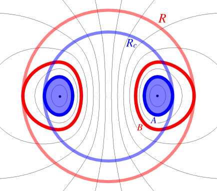
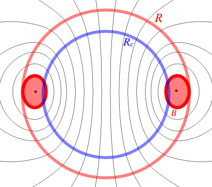
Figure 1: Schematic configurations of mixed poloidal-toroidal magnetic fields. The outer crust and crust-core interface are the red and blue circles labelled $R$ and $R_{\rm c}$ respectively. Left panel: closed field lines in the core — the thick blue field line, labelled A, is the outer-most poloidal field line that is closed in the core, and the red magnetic field line, labelled B, is the outer-most closed field line in the entire star. For the twisted-torus model, toroidal field is confined to the region enclosed by B. The black dots represent the neutral line (the point where the poloidal magnetic field component is zero). Right panel: no closed field lines in the core – the only closed field lines penetrate the crust-core interface, with B being the outer-most closed poloidal field line. Again, the twisted-torus model has toroidal field confined to the region enclosed by B.

As we have already seen, the spindown quasi-equilibrium for a mixed background field, $\mathbf{B}_{0}$, is described by eqn. (14),

$$\mathbf{B}_{{\mathcal{P}}}\cdot\nabla(\varpi b^{\varphi})+\mathbf{b}_{\mathcal{P}}\cdot\nabla(\varpi B^{\varphi}_{0})=4\pi\varpi^{2}\left(\,-\rho_{\rm p}\dot{\Omega}+2{\cal B}\rho_{\rm n}\Omega_{\rm n}\Omega_{\rm np}\,\right).$$ (49)

Since $\mathbf{b}_{\mathcal{P}}$ is axisymmetric, we can introduce a new stream function $\beta(r,\theta)$:

$$\mathbf{b}_{\mathcal{P}}=\nabla\beta\times\nabla\varphi.$$ (50)

Expressed in magnetic coordinates, where $\beta=\beta(\psi,\chi)$,

$$\mathbf{b}_{\mathcal{P}}=\frac{\partial_{\psi}\beta}{h_{\varphi}h_{\psi}}\hat{\chi}-\frac{\partial_{\chi}\beta}{h_{\varphi}h_{\chi}}\hat{\psi}.$$ (51)

We also introduce a stream function ${\cal I}$ for the background toroidal field,

$$B^{\varphi}_{0}={\cal I}\nabla\varphi.$$ (52)

It is well known that for an axisymmetric magnetic equilibrium the two stream functions are related as ${\cal I}={\cal I}(\psi)$ (e.g. Glampedakis et al. (2012)).

In terms of these new functions, we can write (49) as (recall that $B_{\mathcal{P}}=1/h_{\psi}h_{\varphi}$, see Appendix B)

$$\partial_{\chi}T-{\cal I}^{\prime}\partial_{\chi}\beta=4\pi\varpi^{2}h_{\varphi}h_{\chi}h_{\psi}\left(\,-\rho_{\rm p}\dot{\Omega}+2{\cal B}\rho_{\rm n}\Omega_{\rm n}\Omega_{\rm np}\,\right).$$ (53)

It is straightforward to see that (53) breaks down when integrated along a closed field line in the core. Along such a line ${\cal I}^{\prime}$ is constant and therefore the integration leads to

$$0=\oint d\chi\varpi^{2}h_{\varphi}h_{\chi}h_{\psi}\left(\,-\rho_{\rm p}\dot{\Omega}+2{\cal B}\rho_{\rm n}\Omega_{\rm n}\Omega_{\rm np}\,\right),$$ (54)

which is a contradiction. This verifies the assertion discussed earlier in Section 2.2 that closed field lines are incompatible with the assumption of crust-core corotation.

Next, we consider (53) along an open field line. Its integration yields

$$M(\chi,\psi)\equiv T(\chi,\psi)-{\cal I}^{\prime}\beta(\chi,\psi)=-4\pi\dot{\Omega}\int_{0}^{\chi}d\chi^{\prime}h_{\chi^{\prime}}h_{\psi}h_{\varphi}\rho_{\rm p}\varpi^{2}+8\pi{\cal B}\Omega_{\rm np}\Omega_{\rm n}\int_{0}^{\chi}d\chi^{\prime}h_{\chi^{\prime}}h_{\psi}h_{\varphi}\rho_{\rm p}\varpi^{2},$$ (55)

where we have used the assumed equatorial symmetry and anti-symmetry for $b^{r}$ and $b^{\varphi}$, respectively.

For the crust-core torque we have (remember that this is the contribution of the upper hemisphere multiplied by two):

$$N_{\rm cc}=\frac{1}{2\pi}\int_{R_{\rm c}}\frac{dS}{\varpi_{\rm c}}\left[\,\left\{\,M+\partial_{\psi}({\cal I}\beta)\,\right\}\frac{(\hat{r}\cdot\hat{\chi})}{h_{\psi}}-{\cal I}\frac{\partial_{\chi}\beta}{h_{\chi}}(\hat{r}\cdot\hat{\psi})\,\right].$$ (56)

In taking the surface integral, we need to make sure that the range of $\psi$ is limited to the open lines across the crust-core interface. That is, $\psi$ should ‘run’ between the value $\psi_{z}$ of the symmetry axis and $\psi_{A}$ of the line A, see Fig. 1. At the same time, the range for the $\psi$-integration of the terms that depend on the toroidal field ${\cal I}$ is the subset $\psi_{B}<\psi<\psi_{A}$ of the previous range, with $\psi_{B}$ corresponding to the boundary line B of the toroidal field region.

It is straightforward to obtain,

$$N_{\rm cc}=-\bar{I}_{\rm p}\dot{\Omega}+2{\cal B}\Omega_{\rm n}\Omega_{\rm np}\bar{I}_{\rm n}+\int_{\psi_{B}}^{\psi_{A}}d\psi\left[1+\left(\frac{h_{\chi}\partial_{\psi}R_{\rm c}}{h_{\psi}\partial_{\chi}R_{\rm c}}\right)^{2}\,\right]^{1/2}_{\chi_{c}}\left\{\,\partial_{\psi}({\cal I}\beta)(\hat{r}\cdot\hat{\chi})-{\cal I}\partial_{\chi}\beta\frac{h_{\psi}}{h_{\chi}}(\hat{r}\cdot\hat{\psi})\,\right\}_{\chi_{c}},$$ (57)

where we have defined

$$\bar{I}_{\rm x}=4\pi\int_{\psi_{z}}^{\psi_{A}}d\psi\,\left[1+\left(\frac{h_{\chi}\partial_{\psi}R_{\rm c}}{h_{\psi}\partial_{\chi}R_{\rm c}}\right)^{2}\,\right]^{1/2}_{\chi_{\rm c}}(\hat{r}\cdot\hat{\chi})_{\chi_{\rm c}}\int_{0}^{\chi_{\rm c}(\psi)}d\chi h_{\chi}h_{\psi}h_{\varphi}\rho_{\rm x}\varpi^{2}.$$ (58)

This can be compared with the moment of inertia $\tilde{I}_{\rm x}$ appearing in the earlier calculation of the poloidal field with open lines. The difference in the integration limits implies that $\bar{I}_{\rm x}\leq\tilde{I}_{\rm x}$, with the equality holding when there are no closed lines in the core or, equivalently, when the poloidal’s field neutral point is pushed outside into the crust.

So far the discussion in this section applies to the case of an arbitrary twisted torus-like field, but in order to proceed further we make the assumption of a dipole poloidal field ${\cal B}_{\mathcal{P}}$, i.e.

$$\psi=Af(\tilde{r})\sin^{2}\theta,\qquad\tilde{r}=\frac{r}{R},$$ (59)

where for convenience we have taken $f$ to be a dimensionless function. In Appendix C we obtain the following results for the geometric factors appearing in (57) and (58):

$$\left[1+\left(\frac{h_{\chi}\partial_{\psi}R_{\rm c}}{h_{\psi}\partial_{\chi}R_{\rm c}}\right)^{2}\,\right]^{1/2}(\hat{r}\cdot\hat{\chi})=1,\qquad\frac{h_{\psi}}{h_{\chi}}\left[1+\left(\frac{h_{\chi}\partial_{\psi}R_{\rm c}}{h_{\psi}\partial_{\chi}R_{\rm c}}\right)^{2}\,\right]^{1/2}(\hat{r}\cdot\hat{\psi})=\pm\frac{G}{2Af\cos\theta},$$ (60)

where the explicit form of the function $G(r)$ is given in Appendix B. The sign arbitrariness of the second equation comes from the fact that the inner product $\hat{r}\cdot\hat{\psi}$ can switch sign along a given field line (open or closed).

We then have from (57) and (58),

$$\bar{I}_{\rm x}=4\pi\int_{\psi_{z}}^{\psi_{A}}d\psi\,\int_{0}^{\chi_{\rm c}(\psi)}d\chi h_{\chi}h_{\psi}h_{\varphi}\rho_{\rm x}\varpi^{2}\leq I_{\rm x},$$ (61)

and

$$N_{\rm cc}=-\bar{I}_{\rm p}\dot{\Omega}+2{\cal B}\Omega_{\rm n}\Omega_{\rm np}\bar{I}_{\rm n}\\ +{\cal I}(\psi_{A})\beta(\chi_{\rm c},\psi_{A})\mp\frac{G_{\rm c}}{2Af_{\rm c}}\int_{\psi_{B}}^{\psi_{A}}d\psi{\cal I}\frac{(\partial_{\chi}\beta)_{\chi_{c}}}{\cos\theta},$$ (62)

where $G_{\rm c},f_{\rm c}$ are the values of $G,f$ at $r=R_{\rm c}$. We have also used the fact that ${\cal I}(\psi_{B})=0$ for the assumed magnetic field geometry. With the help of (see Appendix B)

$$\chi=G\cos\theta\quad\to\quad\chi_{\rm c}(\psi)=G_{\rm c}\left(\,1-\frac{\psi}{Af_{\rm c}}\,\right)^{1/2},$$ (63)

we can obtain the equivalent expression,

$$N_{\rm cc}=-\bar{I}_{\rm p}\dot{\Omega}+2{\cal B}\Omega_{\rm n}\Omega_{\rm np}\bar{I}_{\rm n}+{\cal I}(\psi_{A})\beta(\chi_{\rm c},\psi_{A})\mp\frac{G_{\rm c}}{2Af_{\rm c}}\int_{\psi_{B}}^{\psi_{A}}d\psi\left[\,1-\frac{\psi}{Af_{\rm c}}\,\right]^{-1/2}{\cal I}(\partial_{\chi}\beta)_{\chi_{\rm c}}.$$ (64)

In order to proceed further, an independent solution of the form $\beta=\alpha_{1}\dot{\Omega}+\alpha_{2}\Omega_{\rm np}\Omega_{\rm n}$ must be provided; such a result can only be obtained by solving the remaining poloidal components of the Euler equation (1). These equations can be found in Appendix D, however, solving them analytically does not appear to be possible.

This difficulty did not crop up in our earlier poloidal field analysis because in that case the $\varphi$-Euler equation, the torque $N_{\rm cc}$ and $b^{\varphi}$ itself decouple from $\mathbf{b}_{\mathcal{P}}$ and the poloidal Euler equations. In practise, this means that a purely poloidal $\mathbf{B}_{0}$ field is compatible with the toroidal spindown ‘mode’ $(b^{\varphi},\mathbf{b}_{\mathcal{P}},\delta\Psi_{\rm p})=(b^{\varphi},0,0)$.

A purely toroidal spindown mode is no longer admissible when $B_{0}^{\varphi}\neq 0$ but, nevertheless, it is still possible to find a mixed toroidal-poloidal mode that would allow a complete calculation of the crust-core torque $N_{\rm cc}$. The desired $\mathbf{b}$ is simply the superposition:

$$\mathbf{b}=b^{r}_{\rm a}\hat{r}+b^{\theta}_{\rm s}\hat{\theta}+b^{\varphi}_{\rm a}\hat{\varphi},$$ (65)

where ‘a’ and ‘s’ stand, respectively, for antisymmetric and symmetric.

As a result of the imposed symmetries we have that (i) the $\sim b^{r}B_{0}^{\varphi}$ term in the crust-core torque (20) integrates to zero and (ii) the second left-hand-side term in (14) is anti-symmetric (as opposed to the other symmetric terms) and therefore should be zero, i.e. $\mathbf{b}_{\mathcal{P}}\cdot\nabla(\varpi B_{0}^{\varphi})=0\to{\cal I}^{\prime}\partial_{\chi}\beta=0$. In other words, this spindown mode is characterized by a poloidal perturbation that points along the background field lines, $\mathbf{b}_{\mathcal{P}}=b^{\chi}\hat{\chi}$. At the same time the perturbation (65) also leads to a pair of non-trivial poloidal Euler equations for $\beta$ and $\Psi_{\rm p}$.

Adopting (65) as a spindown ‘mode’ implies that we can remove all $\beta$-dependence from the general result (62) (or (64)), leaving

$$N_{\rm cc}=-\bar{I}_{\rm p}\dot{\Omega}+2{\cal B}\Omega_{\rm n}\Omega_{\rm np}\bar{I}_{\rm n},$$ (66)

as the main result for the total crust-core torque for the case of a mixed magnetic field. According to this, the magnetic field couples the crust with exactly that portion of the core that is threaded by the open magnetic field lines. Assuming that poloidal field has a neutral point somewhere in the core (as in the left panel of Fig. 1), the toroidal-shaped region between the field lines A and B (i.e. the shaded region in Fig. 1) remains magnetically decoupled and of course makes no contribution to the torque. The same property can be seen to hold true for the more general case represented by eqn. (64). The astrophysical implications of this remarkable result are discussed in the following section.

Finally, it is worth remarking on a fundamental difference between the above argument regarding the crust-core torque and Easson’s no-crust-core corotation argument. We remind the reader that Easson (1979) showed that a crust-core corotation equilibrium cannot exist along closed poloidal field lines in the core, as the governing equations lead necessarily to a mathematical inconsistency when corotation is assumed (see Section 2.2). Our analysis, facilitated by the use of magnetic coordinates, has shown that the closed field lines of poloidal/mixed magnetic fields do not couple at all with the crust and as a result the crust cannot exert any torque on the region occupied by the closed lines. These two anti-corotation arguments are clearly complementary; our analysis explains that closed field lines can violate the corotation assumption as they are decoupled from the crust. This subtle issue may be purely academic; as we discuss below, we expect the spin-lag generated between the open- and closed-field-line regions to render the latter region dynamically unstable, implying crust-core corotation can only be established in the absence of closed field lines in the core.

5 Failure of long-term crust-core corotation: implications

5.1 Incomplete crust-core coupling: how likely is it?

The results obtained in the preceding sections strongly suggest that the extent to which the liquid core can follow the secular spindown of the solid crust is largely decided by the geometry of the magnetic field in the core, in agreement with the original conjecture put forward by Easson (1979). A key question raised in that early work concerned the ‘size’ of the class of magnetic fields that are unable to enforce a full crust-core coupling, and hence allow for the build up of a persistent spin-lag between part of the core and the rest of the star.

This paper provides a definitive answer to that crucial question. As we have seen, an arbitrary dipole poloidal field with no closed field lines in the core does enforce complete crust-core corotation, in agreement with ‘conventional wisdom’. However, the presence of purely poloidal magnetic fields in neutron stars enjoys very little theoretical support since these fields are inherently unstable (e.g. Wright (1973); Flowers & Ruderman (1977); Braithwaite (2007); Lasky et al. (2011)) (the same is true for purely toroidal fields (Tayler, 1973; Braithwaite, 2006)). Instead, hybrid poloidal-toroidal ‘twisted torus’ fields are the ones commonly attributed to realistic neutron stars and the ones that have attracted most theoretical work in the recent years (e.g. Braithwaite & Spruit (2006); Colaiuda et al. (2008); Ciolfi et al. (2009); Mastrano et al. (2011); Glampedakis et al. (2012); Lander & Jones (2012); Ciolfi & Rezzolla (2013); Fujisawa & Kisaka (2014)). Such fields are exemplified by the left-hand panel of Fig. 1: they typically have closed field lines in the core (although the neutral line may be located in the crust for sufficiently strong toroidal components (Ciolfi et al., 2009)) and, as we have shown in Section 4, the part of the core occupied by these lines remains magnetically decoupled from the crust (and the rest of the core).

This result implies that the aforementioned class of magnetic fields is ‘large’, in the sense that such fields should be considered likely to occur in real systems. These include the most commonly used twisted torus models, but not necessarily fields for which the magnetic field is misaligned with the rotation axis (see section 6). In what follows we discuss the spindown evolution of a neutron star endowed with a twisted torus-like magnetic field and speculate on the implications of our results.

5.2 Implications for the magnetic field evolution

To what extent the crust and the core can be interlocked in long-term corotation is most relevant soon after a neutron star’s birth. Assuming a standard cooling scenario, the crust is expected to form approximately a day after the neutron star is formed, when the temperature has dropped to $T\sim\mbox{(few)}\times 10^{9}\,\mbox{K}$ (Shapiro & Teukolsky, 1983). During the same period, the star retains most of its initial kinetic energy (this is true even for newly-born magnetars unless their surface dipole field exceeds approximately $10^{14}-10^{15}\,\mbox{G}$) and therefore most of the subsequent electromagnetic spindown will take place when the star has a well defined solid crust and a liquid core. The onset of neutron superfluidity in the core is likely to ensue much later ($\sim 1\,\mbox{yr}-100\,\mbox{yr}$), when the star has cooled below $T\sim 10^{9}\,\mbox{K}-\mbox{(few)}\times 10^{8}\,\mbox{K}$, respectively (Shternin et al., 2011; Page et al., 2011). On the other hand, the formation of the superconducting proton condensate is expected to take place much earlier, at $T>10^{9}\,\mbox{K}$ (Shapiro & Teukolsky, 1983).

Once the crust is well formed and has begun to be torqued by the anchored magnetic field, two mechanisms come into play in an attempt to enforce crust-core corotation: the magnetic field and hydrodynamical viscous Ekman pumping. The latter mechanism has been extensively discussed in the neutron star literature, most notably in Easson (1979); Abney & Epstein (1996); Melatos (2012), see also Greenspan (1968). As recently emphasized in Melatos (2012), the combined effect of stratification and compressibility in neutron star matter severely inhibits the efficiency of the Ekman mechanism, resulting in corotation timescales much longer than initially anticipated (Abney & Epstein, 1996). For typical neutron stars parameters, a viscous coupling timescale as long as $\sim 10^{3}\,\mbox{yr}$ is expected (Melatos, 2012). The magnetic coupling mechanism is much faster than this (see also our discussion in Section 1); we can therefore frame our discussion without having to consider viscosity, consistent with the model presented in this paper.

A day-old neutron star is likely to start its secular spindown evolution being in stable hydromagnetic equilibrium with a magnetic field geometry that resembles the ones shown in Fig. 1. Consider first the case of the right panel of Fig. 1. In that scenario, the poloidal neutral point is located in the crust, as is the bulk of the toroidal field. The entire core is threaded by open (poloidal and toroidal) field lines and, as we have shown in this paper, the magnetic coupling can enforce corotation between the crust and the total amount of charged fluids in the core. Our analysis and results apply equally well to a system with normal or superfluid neutrons, in the former case the implication being that the magnetic field directly couples all the fluids to the crust, while in the latter case vortex mutual friction is very efficient in enforcing corotation between the superfluid and the protons.

More interesting (and perhaps more probable) is the case of neutron stars ‘starting’ with the magnetic field equilibrium of the left panel of Fig. 1, where the poloidal neutral point and the bulk of the toroidal field are located in the outer core. In such a case, the toroidal-shaped region bounded by the closed line A (depicted as a shaded region in Fig. 1) remains magnetically decoupled to the crust and, as the rest of the star spins down, a spin lag will begin to build up, with the toroidal region retaining its initial ‘fossil’ spin frequency.

It is unlikely that this state of persistent crust-core spin lag can remain dynamically stable for long. The velocity jump in the proton fluid across boundary A will give rise to an increasingly strong azimuthal current sheet $\Delta J\hat{\varphi}$ and an associated poloidal Lorentz force $\Delta J\hat{\varphi}\times\mathbf{B}_{\mathcal{P}}/c$. We would expect $|\Delta J/J|\sim\Delta\Omega/\Omega$ where $\Delta\Omega(t)\sim\dot{\Omega}t$ is the spin lag. This means that the induced Lorentz force can seriously disturb the background equilibrium after a time $t\sim t_{\rm sd}=\Omega/|\dot{\Omega}|$.

The physical conditions along the same boundary field line A are also suitable for the onset of the classical Kelvin-Helmholtz instability. This should take place once the spin lag exceeds the threshold $\Delta\Omega_{\rm KH}\sim v_{\rm A}/R$, where $v_{\rm A}$ is the average Alfvén speed of the local toroidal field $B^{\varphi}_{0}$ (see Chandrasekhar (1981), Chapter XI, p. 507). The corresponding timescale for the onset of the instability, $t_{\rm KH}$, can be estimated to be (here we use canonical values $M=1.4\,M_{\odot}$ and $R=10\,\mbox{km}$ for the stellar mass and radius):

$$\frac{t_{\rm KH}}{t_{\rm sd}}\sim\frac{v_{\rm A}}{\Omega R}\approx 5\times 10^{-2}\left(\frac{B^{\varphi}_{0}}{10^{15}\,\mbox{G}}\right)\left(\frac{P}{10\,\mbox{ms}}\right),$$ (67)

suggesting that it can set in much sooner than the lapse of one spindown timescale. The inclusion of proton superconductivity can significantly raise the above ratio, $v_{\rm A}/\Omega R\approx 0.2\,(B^{\varphi}_{0}/10^{15}\,\mbox{G})^{1/2}(P/10\,\mbox{ms})$, but this is still well below unity provided $P\lesssim 10\,\mbox{ms}$, assuming a magnetar-strength field $B^{\varphi}_{0}$.

We thus have good reason to expect that the initial persistent crust-core spin lag will lead to some kind of magnetohydrodynamic instability after a time (assuming a standard spindown torque, see e.g. Shapiro & Teukolsky (1983))

$$t\lesssim t_{\rm sd}\approx 4.7\,\left(\frac{B_{d}}{10^{15}\,\mbox{G}}\right)^{-2}\left(\frac{P}{10\,\mbox{ms}}\right)^{2}\,\mbox{d},$$ (68)

where $B_{d}$ is the dipole surface field. Among all systems, newly born magnetars appear to be the most favoured ones with respect to the onset of the instability, typically having $t_{\rm sd}\sim 1\mbox{d}-1\,\mbox{yr}$. On the other hand, however, too strongly magnetized and/or too rapidly rotating magnetars will spin down before the formation of their crusts, rendering this discussion moot.

It is beyond the scope of this paper to provide a detailed analysis of the fate of the unstable, super-rotating core region. Nevertheless, we can speculate. Accepting that an initial magnetic equilibrium such as that in the left panel of Fig. 1 is quickly rendered dynamically unstable by the super-rotation of the closed-field-lines region, the magnetic field will try to rearrange itself and find a new stable equilibrium. As long as the neutral line remains in the core, this does not seem viable; any new configuration will still contain closed field line regions which will again lead to a crust-core spin-lag.

Thus, a stable equilibrium is likely to be reached only by the eviction of the neutral line and the attached toroidal field from the core and into the crust. We therefore suggest that the failure of the magnetic field to enforce complete crust-core corotation drives a magnetic field evolution in very young neutron stars akin to moving from the left to the right panel of Fig. 1.

This hypothetical evolutionary scenario sees the crust as the natural depository of toroidal magnetic field and energy initially located in the core. As pointed out earlier, this kind of rotation-driven magnetic field evolution could be especially favoured in magnetars because these magnetized objects experience a rapid spindown soon after the formation of the crust. In other words, and according to the above suggestion, magnetars may have their strong interior toroidal fields pushed into their crusts in $\sim 1\,\mbox{d}-1\,\rm{yr}$ after their birth. This prediction sits well with our theoretical understanding of magnetar thermal properties and seismic activity. A strong, evolving toroidal field in the crust can easily provide the energy required to heat magnetar surfaces to the observed levels (Pons & Geppert, 2007; Kaminker et al., 2006; Ho et al., 2012). The same process could be responsible for fracturing the crust and powering high energy events like magnetar flares (Thompson & Duncan, 2001).

At this stage it is more difficult to speculate on the repercussions of the proposed magnetic field evolution on canonical systems like radio pulsars, or the less magnetized central compact objects (CCOs). The smoother electromagnetic spindown of these objects suggests a much longer spin lag longevity, as $t_{\rm sd}\sim 10^{3}\,\mbox{yr}-10^{4}\,\mbox{yr}$. It should be recalled that the viscous coupling timescale can be of comparable length (Melatos, 2012) and therefore corotation could be achieved regardless of magnetic coupling. It is more likely, however, that the Kelvin-Helmholtz instability will drive magnetic field evolution much earlier than that, especially if the internal toroidal field is comparable to the surface field, i.e. $B^{\varphi}_{0}\sim 10^{12}\,\mbox{G}$; see equation (67). In this latter case, and accounting for superconductivity, the instability would set in after $\sim 1\,\mbox{yr}-100\,\mbox{yr}$.

Although the previous scenario is attractive for all the reasons discussed, it is worth reiterating that it is based mainly in conjecture. However, if for some reason it is not realised, it is possible that a persistent ‘quasi-steady’ turbulent state could be established, driven by shear flows at the interface between the two regions. Turbulent flows in the interiors of neutron stars have many potentially interesting observational consequences (for example see Mastrano & Melatos, 2005; Melatos, 2012, and references therein). Establishing whether the closed-field-line region is evicted from the core or not is a difficult task that we anticipate will require high-resolution numerical simulations to resolve.

Our final remark concerns the role of neutron superfluidity in the evolution of the super-rotating core region. This could be relevant if the persistent spin lag survives until the bulk of the stellar core has become superfluid ($\sim 1\,\mbox{yr}-100\,\mbox{yr}$). Given the previous (very approximate!) instability timescales, this scenario is more likely to be realized in young pulsars, although the low magnetic field/spin frequency end of the magnetar distribution cannot be excluded. The neutron vortex lattice which enables the superfluid to rotate will generally thread both the core region coupled to the crust and the decoupled super-rotating region. The mutual friction force will efficiently couple the neutrons to the protons in both regions, giving rise to a differentially rotating superfluid. In order for this to be possible, the vortices that thread both regions must adapt their spatial distribution and, at the same time, bend in the vicinity of the boundary field line A (see Fig. 1). However, the self-tension of the vortices will prevent this from happening indefinitely. In fact, it might be possible that corotation is established in the entire core under the combined action of the magnetic field and the superfluid vortices. This is an attractive scenario but is one that, as we have pointed out, requires an initially long-lived persistent crust-core spin lag.

6 Concluding discussion

In this paper, we derive conditions for a magnetic field threading the interior of a neutron star to enforce long-term corotation between the slowly-spinning down crust of the star and the superfluid core. We show that a magnetic field with open field lines allows for complete corotation between the two components. However, somewhat counter-intuitively, the presence of any closed field-line region in the core of the star causes that region to be magnetically decoupled from the rest of the star. As the crust and the open-field-line region of the core spin down in unison, a velocity lag will build up between the closed-field-line region and the rest of the star.

Example magnetic field topologies that will generate such persistent spin lags include the popular ‘twisted torus’ configurations, in which toroidal field threads the closed-field-line region of the internal poloidal field (see the left hand panel of Fig. 1). Our results indicate that, soon after the formation of the crust, a young neutron star with, for example, a twisted torus magnetic field will develop a persistent spin lag in the region enclosed by boundary A in the left panel of Fig. 1. The long-term fate of this super-rotating core region is unclear. The velocity difference between the two regions gives rise to a current, and a corresponding Lorentz force that needs to be considered when calculating new magnetohydrostatic equilibria. However, we expect any such equilibria to be unstable to e.g., the classical Kelvin-Helmholtz instability at the interface between the two regions (boundary A in the left-hand panel of Fig. 1). In Section 5, we speculate that any long-term evolution would involve the eviction of the toroidal component of the magnetic field into the crust, thereby allowing the entire core to corotate with the crust.

Fully addressing the question of the long-term fate of the super-rotating core region is a challenging task that requires sophisticated numerical simulations that, we believe, are beyond the capabilities of current techniques. Some difficulties include: simultaneous resolution of the small-scale structure induced by the instabilities at the shear layer and the global magnetic field topology; and the range of timescales in the system, from the secular spin-down and Kelvin-Helmholtz timescales ($\sim$ days – years) down to the Alfvén timescale governing the dynamical adjustments of the magnetic field. We therefore advocate a multipronged approach, include calculations of quasi-static, magnetohydrostatic evolutions to understand the influence of the poloidal Lorentz force on the toroidal-field-line region, as well as full magnetohydrodynamic simulations to understand the relevant instabilities at the shear layer.

Although our analysis makes no particular assumption about the properties of neutron star matter (equation of state, degree of stratification etc.), it does involve two main simplifications with respect to the magnetic field. The first one is the assumption of a dipolar structure for the poloidal field which facilitated the full use of the magnetic coordinates formalism. Of course, these coordinates remain a well-defined notion and can be employed for the description of a general axisymmetric field, but this may come at the price of losing a large part of the analytic elegance of the dipole case. Although we have not pursued this issue further, it is unlikely that any of our conclusions will change for a magnetic field of more general, axisymmetric structure. This may not be true for non-axisymmetric fields where, for example, the poloidal field is misaligned with the stellar rotation axis (Lasky & Melatos, 2013), however we suspect any field topology that admits closed field lines in the core will exhibit the same phenomenology. The second simplification is the use of the ‘classical’ Lorentz magnetic force in the Euler equation. Strictly speaking this is ‘wrong’ given that the bulk of the proton fluid is expected to condense to a superconducting state around the same time as the formation of the crust. It is well known that the magnetohydrodynamics of superconducting neutron stars can be quite different to that of their ordinary matter counterparts (Mendell, 1998; Glampedakis et al., 2011). One of the key differences is the form of the magnetic force, which in a superconducting system originates from the smooth-averaged self-tension of the quantized protonic fluxtubes. Future work should address this approximation of our model by using the full machinery of superconducting magnetohydrodynamics.

Appendix A Crust-core coupling for a non-uniform dipole field.

Here we consider the non-uniform dipole field $f(r)=r^{4}$ combined with the assumption of uniform density. Then, eqn. (28) can be solved with separation of variables, leading to the solution

$$b^{\varphi}(\theta)=\frac{\pi}{A\sqrt{\sin\theta}}\left(\,-\rho_{\rm p}\dot{\Omega}+2{\cal B}\rho_{\rm n}\Omega_{\rm n}\Omega_{\rm np}\,\right)\int_{\theta}^{\pi/2}d\theta^{\prime}\sqrt{\sin\theta^{\prime}}.$$ (69)

Using this result and $B^{r}_{0}=2Ar^{2}\cos\theta$ in the formula for the torque, $N_{\rm cc}$, we have after some rearrangement:

$$N_{\rm cc}=-\tilde{I}_{\rm p}\dot{\Omega}+2{\cal B}\Omega_{\rm n}\Omega_{\rm np}\tilde{I}_{\rm n},$$ (70)

with the effective moments of inertia

$$\tilde{I}_{\rm x}=2\pi R^{5}_{\rm c}\rho_{\rm x}\int_{0}^{\pi/2}d\theta\sin^{2}\theta\frac{\cos\theta}{\sqrt{\sin\theta}}\int_{\theta}^{\pi/2}d\theta^{\prime}\sqrt{\sin\theta^{\prime}}.$$ (71)

On the other hand, the total moment of inertia for each fluid is

$$I_{\rm x}=\int dV\rho_{\rm x}r^{2}\sin^{2}\theta=4\pi\int_{0}^{R_{\rm c}}\int_{0}^{\pi/2}drd\theta r^{4}\sin^{3}\theta\rho_{\rm x}.$$ (72)

For uniform density this simplifies to

$$I_{\rm x}=\frac{8\pi}{15}R_{\rm c}^{5}\rho_{\rm x}.$$ (73)

Our final task is to check the value of the ratio $\tilde{I}_{\rm x}/I_{\rm x}$. We have,

$$\frac{\tilde{I}_{\rm x}}{I_{\rm x}}=\frac{15}{4}\int_{0}^{\pi/2}d\theta\sin^{3/2}\theta\cos\theta\int_{\theta}^{\pi/2}d\theta^{\prime}\sqrt{\sin\theta^{\prime}}.$$ (74)

Direct numerical integration reveals that to numerical precision $\tilde{I}_{\rm x}/I_{\rm x}=1$ which implies a fully corotating core (protons and electrons) with the crust.

Appendix B Magnetic coordinates

For a given axisymmetric poloidal field, $\mathbf{B}_{\mathcal{P}}=\nabla\psi\times\nabla\varphi$, we can set up a system of magnetic coordinates, $\{\psi,\chi,\varphi\}$, where $\chi$ measures distance along a field line (without loss of generality we can set $\chi=0$ at the magnetic equator).

The resulting coordinate system is orthogonal but curvilinear with line element,

$$d\mathbf{r}\cdot d\mathbf{r}=h_{\psi}^{2}\,d\psi^{2}+h_{\chi}^{2}\,d\chi^{2}+h_{\varphi}^{2}\,d\varphi^{2},$$ (75)

where $h_{\psi},h_{\chi},h_{\varphi}$ are all functions of $\psi$ and $\chi$, and it is easy to see that $h_{\varphi}=\varpi$. By construction, $\mathbf{B}_{\mathcal{P}}$ is tangent to $\psi$ surfaces, i.e.,

$$\mathbf{B}_{\mathcal{P}}=B_{0}(\psi,\chi)\hat{\chi}.$$ (76)

The grad operator takes the form (where as always a ‘hat’ denotes a unit vector)

$$\nabla=\frac{\hat{\psi}}{h_{\psi}}\partial_{\psi}+\frac{\hat{\chi}}{h_{\chi}}\partial_{\chi}+\frac{\hat{\varphi}}{h_{\varphi}}\partial_{\varphi}.$$ (77)

We then find,

$$\mathbf{B}_{\mathcal{P}}=\nabla\psi\times\nabla\varphi=\frac{1}{h_{\varphi}h_{\psi}}\hat{\chi}.$$ (78)

For the remainder of the analysis we assume a dipole field, implying the stream function can be expressed in the general form

$$\psi(r,\theta)=Af(\tilde{r})\sin^{2}\theta,$$ (79)

where $\tilde{r}=r/R$. As we have seen, the components of this field in spherical coordinates are

$$B_{0}^{r}=2A\frac{f}{r^{2}}\cos\theta,\qquad B_{0}^{\theta}=-A\frac{f^{\prime}}{Rr}\sin\theta,$$ (80)

where $f^{\prime}=df(x)/dx$.

From this we can obtain the metric component $h_{\psi}$:

$$h_{\psi}(r,\theta)=\frac{r}{A\sin\theta}\left[\,4f^{2}\cos^{2}\theta+(\tilde{r}f^{\prime})^{2}\sin^{2}\theta\,\right]^{-1/2}.$$ (81)

Expressing the line element for the two-sphere in terms of $h_{\psi}$ and $h_{\chi}$, we can obtain three equations

$$\left(h_{\chi}\frac{\partial\chi}{\partial r}\right)^{2}=1-(\tilde{r}f^{\prime})^{2}\sin^{2}\theta\left[\,4f^{2}\cos^{2}\theta+(\tilde{r}f^{\prime})^{2}\sin^{2}\theta\,\right]^{-1},$$ (82)

$$\left(h_{\chi}\frac{\partial\chi}{\partial\theta}\right)^{2}=r^{2}\left\{1-4f^{2}\cos^{2}\theta\left[\,4f^{2}\cos^{2}\theta+(\tilde{r}f^{\prime})^{2}\sin^{2}\theta\,\right]^{-1}\right\},$$ (83)

$$h_{\chi}^{2}\frac{\partial\chi}{\partial r}\frac{\partial\chi}{\partial\theta}=-2\sin\theta\cos\theta r\tilde{r}ff^{\prime}\left[\,4f^{2}\cos^{2}\theta+(\tilde{r}f^{\prime})^{2}\sin^{2}\theta\,\right]^{-1}.$$ (84)

It is straightforward to see that the bottom equation is trivially satisfied by the first two. Simplifying the first two equations and taking square roots,

$$\frac{\partial\chi}{\partial r}=\pm 2f\frac{\cos\theta}{h_{\chi}}\left[\,4f^{2}\cos^{2}\theta+(\tilde{r}f^{\prime})^{2}\sin^{2}\theta\,\right]^{-1/2},$$ (85)

$$\frac{\partial\chi}{\partial\theta}=\pm r\tilde{r}f^{\prime}\frac{\sin\theta}{h_{\chi}}\left[\,4f^{2}\cos^{2}\theta+(\tilde{r}f^{\prime})^{2}\sin^{2}\theta\,\right]^{-1/2}.$$ (86)

Somewhat trivially, $\partial_{r}\chi>0$ for all $\chi(r,\theta)$ for a dipole poloidal field, and we therefore consider only the ‘$+$’ sign in equation (85). On the other hand, $\partial_{\theta}\chi$ can be positive and negative along any given field line. For example, consider field line $A$ in the left hand panel of Fig. 1. As one moves from the innermost equatorial point on $A$ in the clockwise direction, $\partial_{\theta}\chi>0$ until the apex of the field line is reached, at which point $\partial_{\theta}\chi$ changes sign, and becomes negative as one moves further in the clockwise direction. We accordingly introduce $\epsilon=\pm 1,\,0$ into equation (86).

Motivated by solutions in the case when $f(\tilde{r})=\tilde{r}^{a}$ (see below), we search for a coordinate transformation of the form

$$\chi(r,\theta)=G(r)\cos\theta.$$ (87)

Inserting this ansatz into equations (85) and (86) gives respectively

$$\frac{dG}{dr}=\frac{2f}{h_{\chi}}\left[\,4f^{2}\cos^{2}\theta+(\tilde{r}f^{\prime})^{2}\sin^{2}\theta\,\right]^{-1/2},$$ (88)

$$G=-\epsilon r\tilde{r}\frac{f^{\prime}}{h_{\chi}}\left[\,4f^{2}\cos^{2}\theta+(\tilde{r}f^{\prime})^{2}\sin^{2}\theta\,\right]^{-1/2}.$$ (89)

Dividing equation (88) by (89) eliminates the dependence on $\theta$, and gives us a first-order ordinary differential equation for $G$. The formal solution of this equation is

$$G=\exp\left(-\frac{2}{\epsilon}\int d\tilde{r}\frac{f}{\tilde{r}^{2}f^{\prime}}\right),$$ (90)

which can be put back into equation (87), leaving the final coordinate transformation:

$$\chi(r,\theta)=\exp\left(-\frac{2}{\epsilon}\int d\tilde{r}\frac{f}{\tilde{r}^{2}f^{\prime}}\right)\cos\theta.$$ (91)

Inserting this back into equation (82) for the metric coefficient, $h_{\chi}$, yields

$$h_{\chi}(r,\theta)=-\epsilon r\tilde{r}f^{\prime}\exp\left(\frac{2}{\epsilon}\int d\tilde{r}\frac{f}{\tilde{r}^{2}f^{\prime}}\right)\left[\,4f^{2}\cos^{2}\theta+(\tilde{r}f^{\prime})^{2}\sin^{2}\theta\,\right]^{-1/2}.$$ (92)

For a given dipole field, one prescribes $f(r)$, and can derive the full coordinate transformation between spherical polar coordinates and magnetic coordinates using equations (79) and (91).

As an example of this we consider a simple power law, $f(\tilde{r})=\tilde{r}^{a}$, which includes a uniform field ($a=2$) and the ‘standard’ dipole field ($a=4$) as special cases. In this case, the coordinate transformation becomes

$$\psi(r,\theta)=A\tilde{r}^{a}\sin^{2}\theta,\qquad\chi(r,\theta)=C\tilde{r}^{-2/a\epsilon}\cos\theta,$$ (93)

where $C$ is a constant of integration.

Appendix C Some geometric applications of magnetic coordinates

As a first application of our magnetic coordinates, we calculate the infinitesimal surface element $dS$ on a sphere of radius $r_{0}$. This is given by

$$dS=h_{\varphi}d\varphi\left(\,h_{\psi}^{2}d\psi^{2}+h_{\chi}^{2}d\chi^{2}\,\right)^{1/2}.$$ (94)

On the spherical surface we have $d\chi=-(\partial_{\psi}r_{0}/\partial_{\chi}r_{0})d\psi$ and then

$$dS=h_{\varphi}h_{\psi}\left[\,1+\left(\frac{h_{\chi}\partial_{\psi}r}{h_{\psi}\partial_{\chi}r}\right)^{2}\,\right]^{1/2}d\varphi d\psi.$$ (95)

As a second application of the magnetic coordinates, we derive the equation for a circle of radius $r_{0}=r_{0}(\chi,\psi)$. Beginning with the stream function, $\psi=Af(\tilde{r})\sin^{2}\theta$, we use equation (91) to eliminate the $\sin^{2}\theta$ term:

$$\frac{\psi}{A}=f\left(1-\frac{\chi^{2}}{G^{2}}\right),$$ (96)

which is an implicit equation for the circle since $G=G(r_{0})$ and $f=f(r_{0}/R)$. From this we obtain the partial derivatives

$$\frac{\partial r_{0}}{\partial\psi}=\frac{1}{A}\left[\,\frac{f^{\prime}}{R}\left(1-\frac{\chi^{2}}{G^{2}}\right)+2f\chi^{2}\frac{G^{\prime}}{G^{3}}\,\right]^{-1},\qquad\frac{\partial r_{0}}{\partial\chi}=\frac{2f\chi}{G^{2}}\left[\,\frac{f^{\prime}}{R}\left(1-\frac{\chi^{2}}{G^{2}}\right)+2f\chi^{2}\frac{G^{\prime}}{G^{3}}\,\right]^{-1}.$$ (97)

Their ratio is

$$\frac{\partial_{\psi}r_{0}}{\partial_{\chi}r_{0}}=\frac{G}{2Af\cos\theta},$$ (98)

and we also have

$$\frac{h_{\chi}}{h_{\psi}}=-A\sin\theta\frac{\epsilon\tilde{r}_{0}f^{\prime}}{G}.$$ (99)

From these results we find

$$\frac{h_{\chi}}{h_{\psi}}\frac{\partial_{\psi}r_{0}}{\partial_{\chi}r_{0}}=-\frac{\epsilon}{2}\tan\theta\frac{\tilde{r}f^{\prime}}{f}.$$ (100)

In order to make contact with the main body of the paper we also need to calculate the inner product

$$\hat{r}\cdot\hat{\chi}=\frac{B_{0}^{r}}{B_{\mathcal{P}}}=2f\cos\theta[4f^{2}\cos^{2}\theta+(\tilde{r}f^{\prime})^{2}\sin^{2}\theta]^{-1/2}.$$ (101)

We also have

$$\hat{r}\cdot\hat{\psi}=\pm[1-(\hat{r}\cdot\hat{\chi})^{2}]^{1/2}=\pm\tilde{r}f^{\prime}\sin\theta[4f^{2}\cos^{2}\theta+(\tilde{r}f^{\prime})^{2}\sin^{2}\theta]^{-1/2}.$$ (102)

It is then straightforward to verify the identities:

$$(\hat{r}\cdot\hat{\chi})\left[1+\left(\frac{h_{\chi}\partial_{\psi}r_{0}}{h_{\psi}\partial_{\chi}r_{0}}\right)^{2}\,\right]^{1/2}=1,\qquad(\hat{r}\cdot\hat{\psi})\left[1+\left(\frac{h_{\chi}\partial_{\psi}r_{0}}{h_{\psi}\partial_{\chi}r_{0}}\right)^{2}\,\right]^{1/2}=\pm\frac{1}{2}\tan\theta\frac{\tilde{r}f^{\prime}}{f}.$$ (103)

For the example given in Appendix B, $f=\tilde{r}^{a}$, the above formulae reduce to

$$\frac{\partial_{\psi}r_{0}}{\partial_{\chi}r_{0}}=-\frac{Ra}{2AC\cos\theta}\left(\frac{r_{0}}{R}\right)^{-a-2/a\epsilon},\qquad\left(\frac{h_{\chi}\partial_{\psi}r_{0}}{h_{\psi}\partial_{\chi}r_{0}}\right)^{2}=\frac{a^{2}}{4}\tan^{2}\theta,\qquad\hat{r}\cdot\hat{\chi}=2\cos\theta\left[\,4\cos^{2}\theta+a^{2}\sin^{2}\theta\,\right]^{-1/2},$$ (104)

and from these the identity (103) follows directly.

Appendix D The poloidal Euler equations

The poloidal component of the perturbed Euler equation (1) is (after omitting the Coriolis term and the unimportant $\sim{\cal B}^{\prime}$ mutual friction term):

$$4\pi\rho_{\rm p}\nabla_{P}\Psi_{p}=-\nabla_{P}\left(\mathbf{B}_{0}\cdot\mathbf{b}\right)+\left[\,(\mathbf{b}\cdot\nabla)\mathbf{B}_{0}+(\mathbf{B}_{0}\cdot\nabla)\mathbf{b}\,\right]_{P}.$$ (105)

Using magnetic coordinates, we have for the individual terms of (105)

$$[(\mathbf{b}\cdot\nabla)\mathbf{B}_{0}]_{P}=\hat{\psi}\left[\frac{B_{P}}{h_{\psi}h_{\chi}}\left(b_{\psi}\partial_{\chi}h_{\psi}-b_{\chi}\partial_{\psi}h_{\psi}\right)-\frac{B^{\varphi}b^{\varphi}}{h_{\psi}h_{\varphi}}\partial_{\psi}h_{\varphi}\right]+\hat{\chi}\left[\mathbf{b}\cdot\nabla B_{P}-\frac{B^{\varphi}b^{\varphi}}{h_{\chi}h_{\varphi}}\partial_{\chi}h_{\varphi}\right],$$ (106)

$$[(\mathbf{B}_{0}\cdot\nabla)\mathbf{b}]_{P}=\hat{\psi}\left[\,\mathbf{B}_{0}\cdot\nabla b_{\psi}-\frac{B_{P}b_{\chi}}{h_{\psi}h_{\chi}}\partial_{\psi}h_{\chi}-\frac{B^{\varphi}b^{\varphi}}{h_{\psi}h_{\varphi}}\partial_{\psi}h_{\varphi}\,\right]+\hat{\chi}\left[\,\mathbf{B}_{0}\cdot\nabla b_{\chi}+\frac{B_{P}b_{\psi}}{h_{\psi}h_{\chi}}\partial_{\psi}h_{\chi}-\frac{B^{\varphi}b^{\varphi}}{h_{\chi}h_{\varphi}}\partial_{\chi}h_{\varphi}\,\right],$$ (107)

and

$$\nabla_{P}\left(\mathbf{B}_{0}\cdot\mathbf{b}\right)=\frac{\hat{\psi}}{h_{\psi}}\partial_{\psi}\left(B^{\varphi}b^{\varphi}+\frac{\partial_{\psi}\beta}{h^{2}_{\psi}h^{2}_{\varphi}}\right)+\frac{\hat{\chi}}{h_{\chi}}\partial_{\chi}\left(B^{\varphi}b^{\varphi}+\frac{\partial_{\psi}\beta}{h^{2}_{\psi}h^{2}_{\varphi}}\right).$$ (108)

Recalling the expressions,

$${\cal T}=\varpi b^{\varphi},\quad B_{\varphi}^{0}={\cal I}\nabla\varphi,\quad\mathbf{b}_{\mathcal{P}}=\nabla\beta\times\nabla\varphi,$$ (109)

then after some straightforward manipulations we arrive at the following components of (105)

$$-4\pi\rho_{\rm p}\partial_{\psi}\Psi_{\rm p}=\partial_{\psi}\left(\frac{T{\cal I}}{h_{\varphi}^{2}}+\frac{\partial_{\psi}\beta}{h_{\psi}^{2}h_{\varphi}^{2}}\right)+\frac{1}{(h_{\chi}h_{\varphi})^{2}}\left(\,\partial^{2}_{\chi}\beta-K_{\chi}\partial_{\chi}\beta+2T{\cal I}\frac{h^{2}_{\chi}}{h_{\varphi}}\partial_{\psi}h_{\varphi}+2\frac{h_{\chi}}{h_{\psi}^{2}}\partial_{\psi}h_{\psi}\partial_{\psi}\beta\,\right),$$ (110)

$$-4\pi\rho_{\rm p}\partial_{\chi}\Psi_{\rm p}=\partial_{\chi}\left(\frac{T{\cal I}}{h_{\varphi}^{2}}+\frac{\partial_{\psi}\beta}{h_{\psi}^{2}h_{\varphi}^{2}}\right)-\frac{1}{(h_{\psi}h_{\varphi})^{2}}\left(\,\partial_{\chi}\partial_{\psi}\beta+K_{\psi}\partial_{\chi}\beta-2T{\cal I}\frac{h^{2}_{\psi}}{h_{\varphi}}\partial_{\chi}h_{\varphi}\,\right),$$ (111)

where

$$K_{\chi}=\frac{\partial_{\chi}h_{\varphi}}{h_{\varphi}}+\frac{\partial_{\chi}h_{\chi}}{h_{\chi}}-\frac{\partial_{\chi}h_{\psi}}{h_{\psi}},\qquad K_{\psi}=\frac{\partial_{\psi}h_{\varphi}}{h_{\varphi}}+\frac{\partial_{\psi}h_{\psi}}{h_{\psi}}-\frac{\partial_{\psi}h_{\chi}}{h_{\chi}}.$$ (112)

References

- Abney & Epstein (1996) Abney M., Epstein R.I., 1996, J. Fluid. Mech., 312, 327
- Akgün et al. (2013) Akgün T., Reisenegger A., Mastrano A., Marchant P., 2013, MNRAS, 433, 2445
- Alpar, Langer & Sauls (1984) Alpar M. A., Langer S. A., Sauls J. A., 1984, ApJ, 282, 533
- Andersson et al. (2006) Andersson N., Sidery T., Comer G. L., 2006, MNRAS, 368, 162
- Braithwaite & Spruit (2006) Braithwaite J., Spruit H. C., 2006, A&A, 450, 1097
- Braithwaite & Nordlund (2006) Braithwaite, J., Nordlund A., 2006, A&A, 450, 1077
- Braithwaite (2006) Braithwaite J., 2006, A&A, 453, 687
- Braithwaite (2007) Braithwaite J., 2007, A&A, 469, 275
- Chandrasekhar (1981) Chandrasekhar S., 1981, Hydrodynamic and Hydromagnetic Stability, Dover Press, New York
- Ciolfi et al. (2009) Ciolfi R., Ferrari V., Gualtieri L., Pons J. A., 2009, MNRAS, 397, 913
- Ciolfi & Rezzolla (2013) Ciolfi R., Rezzolla L., 2013, MNRAS, 435, L43
- Colaiuda et al. (2008) Colaiuda A., Ferrari V., Gualtieri L., Pons J. A., 2008, MNRAS, 385, 2080
- Easson (1979) Easson I., 1979, ApJ, 233, 711
- Ferraro (1954) Ferraro V. C. A., 1954, ApJ, 119, 407
- Flowers & Ruderman (1977) Flowers E., Ruderman M. A., 1977, ApJ, 215, 302
- Fujisawa & Kisaka (2014) Fujisawa K., Kisaka S., 2014, MNRAS, 445, 2777
- Glampedakis et al. (2011) Glampedakis K., Andersson N., Samuelsson L., 2011, MNRAS, 410, 805
- Glampedakis et al. (2012) Glampedakis K., Andersson N., Lander S. K., 2012, MNRAS, 420, 1263
- Greenspan (1968) Greenspan H. P., 1968, The Theory of Rotating Fluids, Cambridge University Press, Cambridge
- Hall & Vinen (1956a) Hall H. E., Vinen W. F., 1956, Proc. R. Soc, London A, 238, 204
- Hall & Vinen (1956b) Hall H. E., Vinen W. F., 1956, Proc. R. Soc. London A, 238, 215
- Ho et al. (2012) Ho W. C. G., Glampedakis K., Andersson N., 2012, MNRAS, 422, 2632
- Kaminker et al. (2006) Kaminker A. D., Yakovlev D. G., Potekhin A. Y., Shibazaki N., Shternin P. S., Gnedin O. Y. 2006, MNRAS, 371, 477
- Lander & Jones (2012) Lander S. K., Jones D. I., 2012, MNRAS, 424, 482
- Lasky et al. (2011) Lasky P. D., Zink B., Kokkotas K. D., Glampedakis K., 2011, ApJ, 735, L20
- Lasky & Melatos (2013) Lasky P. D., Melatos, A. 2013, Phys. Rev. D, 88, 103005
- Mastrano & Melatos (2005) Mastrano A., Melatos A., 2005, MNRAS, 361, 927
- Mastrano et al. (2011) Mastrano A., Melatos A., Reisenegger A., Akgün T., 2011, MNRAS, 417, 2288
- Melatos (2012) Melatos A., 2012, ApJ, 761, 32
- Mendell (1998) Mendell G., 1998, MNRAS, 296, 903
- Mitchell et al. (2015) Mitchell, J. P., Braithwaite, J., Reisenegger, A., Spruit, H., Valdivia, J. A., Langer, N., 2015, MNRAS, 447, 1213
- Pons & Geppert (2007) Pons J. A., Geppert U., 2007, A&A , 470, 303
- Page et al. (2011) Page D., Prakash M., Lattimer J. M., Steiner A. W., 2011, Phys. Rev. Lett., 106, 081101
- Shapiro & Teukolsky (1983) Shapiro S. L., Teukolsky S. A., 1983, Black Holes, White Dwarfs, and Neutron Stars. Wiley, New York
- Shternin et al. (2011) Shternin P. S., Yakovlev D. G., Heinke C. O., Ho W. C. G., Patnaude D. J., 2011, MNRAS, 412, L108
- Tayler (1973) Tayler R. J., 1973, MNRAS, 161, 365
- Thompson & Duncan (2001) Thompson C., Duncan R. C., 2001, ApJ, 561, 980
- Wright (1973) Wright G. A. E., 1973, MNRAS, 162, 339