Joint Ranging and Clock Parameter Estimation by Wireless Round Trip Time Measurements

Abstract

In this paper we develop a new technique for estimating fine clock errors and range between two nodes simultaneously by two-way time-of-arrival measurements using impulse-radio ultra-wideband signals. Estimators for clock parameters and the range are proposed that are robust with respect to outliers. They are analyzed numerically and by means of experimental measurement campaigns. The technique and derived estimators achieve accuracies below $1$ Hz for frequency estimation, below $1$ ns for phase estimation and $20$ cm for range estimation, at $4$ m distance using $100$ MHz clocks at both nodes. Therefore, we show that the proposed joint approach is practical and can simultaneously provide clock synchronization and positioning in an experimental system.
Keywords: clock synchronization, range estimation, robust estimators, ultra-wideband

I Introduction

A common time reference among nodes along with node positioning enables coordination in time and space domains. By such coordination the nodes can execute tasks efficiently in internet-of-things (IOT), machine-to-machine (M2M) communication, or similar scenarios [1, 2, 3]. In certain scenarios time synchronization among nodes is necessary for positioning. Specifically, it is needed in positioning techniques where time of arrival (TOA) measurements are required and measurements are performed using a clock. As an example, in the commercially available Ubisense system, sensor nodes are synchronized using cable in order to perform time difference of arrival (TDOA) measurements of ultra-wideband (UWB) pulses from tag nodes [4]. In these types of systems, replacing the cabling with wireless synchronization will reduce the installation cost in stationary environments and increase in flexibility will open up new mobile applications. Positioning and effects of clock parameter mismatch have been addressed jointly before in [5, 6, 7] and the references therein. In [5], optimal algorithms were derived for joint positioning and synchronization with anchor uncertainty in position and time. In [6], the authors proposed distributed algorithms for positioning and synchronization in UWB ad-hoc networks. In [7], the effect of clock skew was discussed and estimators for TDOA-based positioning were formulated. A few recent works on joint ranging and clock synchronization are mentioned in [8, 9, 10, 11]. In [9], authors have proposed a network wide clock synchronization and ranging mechanism by pairwise timestamp measurements aided with passive listening. In [10], authors have proposed clock synchronization and localization along with a low cost testbed for its demonstration.

Our main contribution in this paper lies in suggesting a measurement mechanism which provides information about clock parameters and range between nodes. Further, we propose joint estimators to precisely estimate range and clock parameters from the measurements. The estimated range can subsequently be used for positioning using standard techniques [12, 13, 14]. Such an approach would simplify physical infrastructure and obviate the need for e.g. laying cables for synchronization in positioning systems.

Similarly, wireless clock synchronization can be useful in several other applications; which either presently rely on wired synchronization or work asynchronously but exhibit performance loss in the absence of synchronization. For instance, many packet-based radio systems operate asynchronously and suffer packet collisions. Joint positioning and time synchronization can help reduce such losses in a network. Traditionally, time synchronization is a necessity for a variety of networks. Network time protocol (NTP) is a well-known mechanism to synchronize clocks over the internet [15]. Similarly, time synchronization protocol for sensor networks (TPSN) is in use [16]. In the reference broadcast synchronization (RBS) protocol, time synchronization is achieved by broadcast beacon and receiver timestamp exchanges [17]. In all these network synchronization mechanisms, the clocks are eventually synchronized between two nodes in a network. In this paper, by contrast, we avoid timestamp exchanges, and hence communication overhead, using round-trip time (RTT) measurements. This enables simultaneous estimation of the clock parameters and range between two nodes.

To achieve high accuracy in wireless clock synchronization it is necessary to estimate the delay arising from the signal propagation time between nodes. Here we consider using UWB as the wireless technology and demonstrate results using a UWB-based radio with a very accurate time measuring device or chronometer. Our previous work has demonstrated time measurement precision up to $50$ ps using a time-to-digital converter (TDC) [18]. Furthermore, usage of UWB in very accurate range and position estimation is already well known [12, 13, 6, 19]. Under line of sight conditions the signal propagation delay is directly proportional to the distance between the nodes. Estimating this delay therefore enables ranging as a by product of clock synchronization.

Very few clock parameter estimation results have been verified experimentally in the literature. In [17], measurements were captured using Berkeley motes and logic analyzers and verified offline by synchronization algorithms. The timescale and accuracy in these experiments are in microseconds. Whereas, in our proposed system the timescale and accuracy is in the order of a nano-second, as shown in subsequent sections. In [20], a timestamping system for temporal information dissemination is proposed achieving sub-nanosecond accuracy with UWB pulses. The timestamping system is integrated in a ZigBee platform for wireless sensor networks. However, in [20], one-way time-of-arrival (TOA) is considered, and range estimation is not supported, differently from our proposed technique.

In the literature various theoretical models and methods have been discussed for clock synchronization over wireless networks, cf. [21, 22, 23]. In [22], authors have suggested message-passing methods for network clock estimation. The relative clock model between two clocks adopted in next section is discussed in [23] in greater detail. In [24], the Cramér-Rao bounds were derived on the parameters for this clock model. In subsequent sections we will propose the usage of a clocked delay in the slave node. In our previous work, the generated delay is assumed to be fixed and analog [14, 25, 26]. Here, by contrast, we turn the clock into a delay-generating device producing informative measurements.

Since the proposed technique estimates the range between a master and a slave node, it can be used as a fundamental building block of scalable and cooperative distance-based techniques for network positioning. Specifically, an example of a widely-used technique exploiting node-to-node ranging is based on multi-dimensional scaling (MDS) [27]. Furthermore, cooperative message-passing methods based on Bayesian networks have been developed in [12], and experimentally evaluated on a UWB ranging platform in [28]. An analysis and implementation of such methods is beyond of the scope of the present paper.

The remainder of the paper is organized as follows: Section II describes the considered system model for the paper. In section II-B, the clock parameter measurement mechanism is introduced. This section also introduces the measurement model. In section III, estimators are proposed for estimating clock parameters and range from the measurements. Section IV is composed of a numerical evaluation of the model proposed in section II. Section V provides results from experimental setup and performance of estimators on the acquired data. In section VI we conclude the paper.

Notation: $\mathbf{1}$ denotes a column vector of $1$s. $\mathbf{a}\odot\mathbf{b}$ is the element-wise, or Hadamard, product between vectors $\mathbf{a}$ and $\mathbf{b}$. $\mathbf{x}^{1/2}$ is the element-wise square-root of vector $\mathbf{x}$. $\|\mathbf{x}\|_{\mathbf{W}}=\sqrt{\mathbf{x}^{\top}\mathbf{W}\mathbf{x}}$ where $\mathbf{W}$ is a positive semidefinite matrix. The modulus function is written compactly as $\text{mod}_{y}(x)\triangleq\text{modulo}(x,y)$.

Figure 1: Principle of operation of the considered system: the master node sends a PING signal and the slave node responds. The master node is equipped with a time-to-digital converter capable of measuring the round-trip-time.

II System Model and Problem Formulation

In this section, we first describe the principle of operation of the considered system, then we illustrate the proposed clock measurement mechanism. Subsequently, we define the related signal model and present a basic estimator of the parameters of interest, based on existing literature.

II-A Principle of Operation: Round-Trip Time

We consider two nodes equipped with a wireless transmitter and a receiver. One being called the master and the other called slave [18]. We assume that the master node is capable of measuring the time interval between the transmission of a Ping signal and the reception of a Respond signal, sent by the slave, after a predetermined delay. A conceptual overview is given in Fig. 1. This time interval is denoted as the round-trip-time (RTT) which we express as a function $\tilde{y}$ of the unknown range between the master and slave $\rho$ and the delay $\delta$

$$\tilde{y}=\delta+\frac{2}{c}\rho,$$ (1)

where $c$ is the speed of light in meters per second. Conventionally, the delay is an ideal analog implementation and known at the master, cf. [14, 18]. Here, however, we assume that all timed events are based on local clocks at each node. As we will show below, this enables the joint estimation of both range and parameters for clock synchronization.

Time is measured using a clock by counting a number of periods of the clock signal

$$C_{0} = \frac{n}{f_{0}}+\varphi$$

where $n$ is the number of clock cycles, $f_{0}$ is the nominal clock frequency and $\varphi\in[0,1/f_{0})$ is the initial phase of the clock when the measurement begins. Any fractional deviation from the nominal clock frequency is termed as skew of the clock, represented usually as $\alpha>0$. Time is measured using a skewed clock, expressed in the nominal frequency $f_{0}$ as

$$C = \alpha\frac{n}{f_{0}}+\varphi,$$

and the actual frequency $f$ deviates from nominal clock frequency given by $\alpha=f_{0}/f$. Equivalently the above model is widely used as [29, 30, 7]:

$$C = \alpha t+\varphi\,,$$

For simplicity and to establish the notation, let us first consider a standard linear clock model of the observed times at master and slave nodes,

$$C_{m} = \alpha_{m}t+\varphi_{m}$$

and

$$C_{s} = \alpha_{s}t+\varphi_{s},$$

where $\alpha_{m}$ and $\alpha_{s}$ denote their clock skew with respect to nominal frequency $f_{0}$ and $\varphi$ is the initial phase offset.

The clock parameters are assumed time-invariant [24]. If $f_{m}$ and $f_{s}$ denote the clock frequencies at the master and slave, then we define the frequency difference $f_{d}\triangleq f_{m}-f_{s}$. The relative clock skews will then be parameterized by $f_{d}$ as $\alpha_{s}/\alpha_{m}=f_{m}/f_{s}=f_{m}/(f_{m}-f_{d})$. The time observed at the slave $C_{s}$ can then be expressed relative to a reference, i.e. the master node clock $C_{m}$,

$$\begin{split}C_{s}&=\alpha_{s}\left(\frac{C_{m}-\varphi_{m}}{\alpha_{m}}\right)+\varphi_{s}\\ &=\frac{\alpha_{s}}{\alpha_{m}}C_{m}+\left(\varphi_{s}-\frac{\alpha_{s}}{\alpha_{m}}\varphi_{m}\right)\\ &=\left(\frac{f_{m}}{f_{m}-f_{d}}\right)C_{m}+\frac{\phi}{2\pi(f_{m}-f_{d})},\end{split}$$ (2)

where the second term is the relative clock offset in seconds and we correspondingly define the relative clock offset in radians $\phi$ as

$$\phi\triangleq 2\pi(f_{m}-f_{d})\left(\varphi_{s}-\frac{\alpha_{s}}{\alpha_{m}}\varphi_{m}\right)\in[0,2\pi).$$

This model is illustrated in Fig. 2.

Figure 2: Relative clock error models, $(C_{m},C_{s})$ in (2) $\alpha_{s}/\alpha_{m}$ denotes the clock skew and $\phi$ initial phase in radians.

Given that $C_{m}$ is the reference clock, $f_{m}$ is known and to perform synchronization of master and slave clocks, only estimation of $f_{d}$ and $\phi$ is necessary [31].

If we assume that the slave generates the delay by counting a fixed and known number of clock cycles, equivalent to quantization in the time domain, the nominal delay $\delta_{0}$ becomes dependent on the frequency difference and can be written as

$$\begin{split}\delta_{0}(f_{d})&=\frac{\lfloor(C^{\prime}_{s}-C_{s})(f_{m}-f_{d})\rfloor}{f_{m}-f_{d}}\,,\end{split}$$

where $C_{s}$ and $C^{\prime}_{s}$ denote the time of reception of the Ping and transmission of the Respond signal at the slave.

On the other hand, the master is equipped with a TDC, and is therefore able to measure time intervals with a much higher resolution than its clock period. Based on this mechanism, which we will describe in more detail below, the time measured at the master is given by an integer number of slave clock cycles (i.e. $\delta_{0}$) plus a remainder term, which is naturally modeled by a periodic modulus operation. In the following subsection we present a model of this term, denoted $h(t;f_{d},\phi)$ which is dependent on the unknown clock parameters $f_{d}$ and $\phi$. Therefore, we can write the delay as

$$\delta=\delta_{0}(f_{d})+h(t;f_{d},\phi)$$ (3)

and in combination with (1) the round-trip-time measurements will be informative of the range $\rho$ to the slave but also of the relative clock parameters of the slave, $f_{d}$ and $\phi$, via $\delta$.

II-B Clock Measurement Mechanism

Assuming the frequency difference is small, i.e. $f_{d}\ll f_{m}$, we can neglect the dependence of $\delta_{0}$ on $f_{d}$ since $f_{s}=f_{m}-f_{d}\simeq f_{m}$ and thus we can approximate $\delta_{0}$ as a known constant, i.e.

$$\delta_{0}\simeq\frac{\lfloor(C^{\prime}_{s}-C_{s})f_{m}\rfloor}{f_{m}}\,.$$

Similarly, (3) can be approximated at a specific time instant $t$ as

$$\begin{split}\delta&=\frac{\lfloor(C^{\prime}_{s}-C_{s})(f_{m}-f_{d})\rfloor}{f_{m}-f_{d}}+\frac{1}{2\pi(f_{m}-f_{d})}\text{mod}_{2\pi}(f_{d}t+\phi)\\ &\simeq\delta_{0}+\frac{1}{2\pi f_{m}}\text{mod}_{2\pi}(f_{d}t+\phi)\end{split}$$ (4)

where periodic modulus operation represents the remainder and is dependent on the clock offset and frequency difference. We now illustrate how the remainder term appears at the master node. Consider the following example based on the events described in Fig. 1:

Figure 3: A space-time diagram depicting the clock edges (vertical arrows) at the slave (top row) and master (bottom row). The diagram relates the quantities in (1) and (3). Specifically, the remainder term $h(t)$ in (3) is highlighted.

1. Master sends a Ping pulse on a positive edge of clock, TDC receives the Start signal instantly and starts measuring time.

2. On receiving the pulse, slave starts the delay generation from subsequent positive edge of its own clock.

3. Slave sends Response after the delay $\delta_{0}$ (say, two clock cycles in this example)

4. Master receives the Response, TDC gets the Stop signal and measures the RTT.

This sequence of events is also illustrated in the space-time diagram of Fig. 3 where the remainder term $h(t)$ is highlighted. The master repeats the above transmission procedure with a fixed periodicity. The result is illustrated in Fig. 4 which shows the role of the clock in repeated pings.

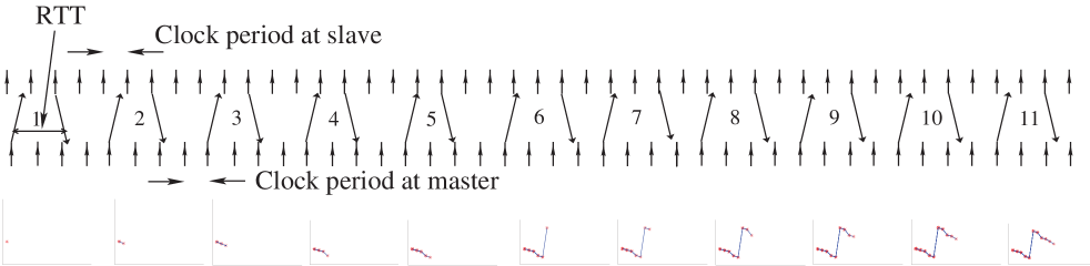
Figure 4: A diagram depicting the clock mechanism. Note that the RTT measurements, plotted below, vary depending on the shift of the slave clock edge relative to the master clock.

At instance ‘5’ Ping from master is received by slave at a clock edge and hence results in smallest RTT. Whereas, at instance ‘6’ slave receives Ping narrowly after the clock edge and hence waits nearly a full clock duration to start its delay count of a clock cycle. This results in largest RTT measurement at master. As can be seen, the clock offset and frequency results in a perodic time-varying remainder term $h(t)$ with a sawtooth-like waveform corresponding to the modulus function that follows from rounding.

In addition to the effect of the rounding operation, the remainder term in (4) is also subject to zero-mean random clock jitter, which we denote $v$. At measurement time instant $t_{i}$ we therefore model the remainder as

$$h(t_{i};f_{d},\phi)=\frac{T_{m}}{2\pi}\text{mod}_{2\pi}(f_{d}t+\phi+v(t_{i})),$$ (5)

where $T_{m}=1/f_{m}$. Finally, inserting (5) into (3) under $f_{d}\ll f_{m}$, (1) results in the following the RTT measurement model at time $t_{i}$:

$$y(t_{i})=\frac{T_{m}}{2\pi}\text{mod}_{2\pi}(f_{d}t_{i}+\phi+v(t_{i}))+\delta_{0}+\frac{2}{c}\rho+n(t_{i}),$$ (6)

where $n(t_{i})$ denotes zero-mean measurement noise. Figure 5 shows a measurement capture of above phenomena on our flexible UWB radio test-bed [18]. In Section V-E we validate the model (6) by means of residual analysis, justifying the approximations used above for the considered experimental setup.

II-C Signal Model and Measurements

Let $\mathbf{y}=[y(t_{1})\>\cdots\>y(t_{N})]^{\top}\in\mathbb{R}^{N}$ and $\mathbf{t}=[t_{1}\cdots\>t_{N}]^{\top}\in\mathbb{R}^{N}$ be the vector of $N$ measurements and time instances, respectively. Then model (6) can be written compactly in vector form:

$$\mathbf{y}=\mathbf{h}(f_{d},\phi,\mathbf{v})+\delta_{0}\mathbf{1}+\frac{2\rho}{c}\mathbf{1}+\mathbf{n}\,,$$ (7)

where

$$\mathbf{h}(f_{d},\phi,\mathbf{v})\triangleq\frac{T_{m}}{2\pi}\text{mod}_{2\pi}(f_{d}\mathbf{t}+\phi\mathbf{1}+\mathbf{v})\,.$$

The vectors $\mathbf{v}$ and $\mathbf{n}$ contain the random noise terms with unknown variances $\sigma^{2}_{v}$ and $\sigma^{2}_{n}$, respectively. The goal is to estimate $\rho$, $f_{d}$ and $\phi$ from $\mathbf{y}$.

Central to RTT measurement procedures is the device called time-to-digital converter (TDC) as is shown in Fig. 1. Commercially available TDCs can measure time with resolution up to $50$ ps [32]. As shown in Fig. 1, TDC measures the time difference between two events and thus measures RTT. The TDC has its own clock for coarse counting [32].

Here we wish to highlight a few important features:

• Measurement model (7) arises from sampling the slave clock over a wireless medium and measuring the relative clock drift using a TDC at master node.

• No timestamping and hence no data transfer is required between master and slave devices.

• Traditionally, clock parameters are estimated as shown in Fig. 2, where measured time monotonically increases. Long time measurements using a clock require high accuracy. Whereas, RTT measurements as seen in Fig. 5 require short time measurements, hence clock accuracy and stability is a lesser concern. When measuring smaller time duration the TDC clock skew is assumed to be negligible.

• Clock parameter information is available in the time domain as well as the frequency domain. The latter fact facilitates extracting information using frequency-based methods.

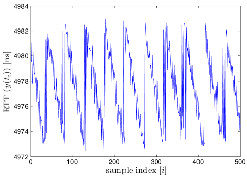
Figure 5: Experimental data record showing the “sawtooth” behavior of the RTT measurements. The data was obtained with the master and slave antennas placed 0.5 m apart, $\delta_{0}=4900$ ns.

Next, we introduce a conventional estimator for estimating $f_{d}$, $\phi$ and $\rho$ by unwrapping the saw-tooth measurement (7); an early work is [29], cf. discussion in [33, 24].

II-D Unwrapped Least Squares (ULS)

We consider the model in (6) and formulate a three-step unwrapped least-squares method (ULS). First, by approximating the arithmetic average of the modulus term in (6) as the amplitude of the sawtooth-like waveform, $T_{m}/2$, we obtain

$$\bar{y} =\frac{1}{N}\sum^{N}_{i=1}y(t_{i})$$

$$\simeq\frac{T_{m}}{2}+\delta_{0}+\frac{2\rho}{c}+\frac{1}{N}\sum^{N}_{i=1}n(t_{i}).$$

From this we form an approximate least-square estimate of the range

$$\hat{\rho} =\operatorname*{arg\,min}_{\rho}\;\left(\bar{y}-\frac{T_{m}}{2}-\delta_{0}-\frac{2\rho}{c}\right)^{2}$$

$$=\frac{c}{2}\left(\bar{y}-\frac{T_{m}}{2}-\delta_{0}\right)\,.$$

Then, we normalize the measurements $y(t_{i})$ to the $\left[-\pi,\pi\right)$-interval as follows:

$$z(t_{i})\triangleq\frac{2\pi}{T_{m}}\left(y(t_{i})-\bar{y}\right)\,.$$

Next, we apply a ‘phase-unwrapping’ algorithm, denoted by $\mathcal{U}(\mathbf{z})$ where $\mathbf{z}=[z(t_{1})\cdots z(t_{N})]^{\top}$ [24, 29, 34]. This algorithm adds multiples of $\pm 2\pi$ rad to the phase when the absolute difference between consecutive elements is greater than $\pi$ rad. Finally, we obtain $\hat{\phi}$ and $\hat{f}_{d}$ by solving the following linear least-squares problem on the unwrapped samples:

$$\begin{split}[\hat{f}_{d},\hat{\phi}]&=\operatorname*{arg\,min}_{f_{d},\>\phi}\>\left\|\mathcal{U}(\mathbf{z})-f_{d}\mathbf{t}-\phi\mathbf{1}\right\|^{2}_{2}.\end{split}$$ (8)

Whilst the ULS estimator is computationally efficient, erroneously unwrapped samples by $\mathcal{U}(\cdot)$ which occur in poor signal conditions lead to performance degradation.

Furthermore, as formulated it is not robust with respect to noise outliers and its estimates may deteriorate significantly. The presence of outliers is a common issue in practical wireless measurement systems. As an evaluation example, the wireless localization scenario is considered in [35]. In such a scenario, outliers in the time-of-arrival measurements are present due to propagation channel conditions, and robust regression techniques are employed for the purpose of reducing the adverse impact of outliers on localization performance.

III Proposed Estimators

In view of the limitations of the unwrapped least squares approach described above, we develop two alternative methods to estimate the offset frequency $f_{d}$, offset phase $\phi$ and range $\rho$ in (7).

III-A Periodogram and Correlation Peaks (PCP)

In the first approach we exploit the periodicity of the signal model (6) to obtain a frequency estimate. Using the periodogram [36] we can compute an estimate up to an unknown sign,

$$\check{f}_{d}=\operatorname*{arg\,max}_{f_{d}\in F}\;\left|\sum^{N}_{i=1}y(t_{i})e^{-j2\pi f_{d}t_{i}}\right|^{2},$$

where $F\subset[0,f_{\text{max}}]$ is a uniform grid of frequencies. Under uniform sampling, the estimate can be computed efficiently using the fast Fourier transform. Note that $f_{d}$ determines the slope of the periodic sawtooth waveform in (6), cf. Fig. 5. The sign of $f_{d}$ can be resolved jointly with phase estimation by correlating the observed signal with sawtooth waveforms based on $\check{f}_{d}$ and $-\check{f}_{d}$, corresponding to positive and negative slopes.

Then using the estimate $\check{f}_{d}$ a waveform $\mathbf{p}(\phi,s)=\text{mod}_{2\pi}(s\check{f}_{d}\mathbf{t}+\phi\mathbf{1})$ is generated, for a fixed frequency sign $s=\{-1,1\}$ and nominal phase $\phi$. The phase estimate, and the resolved sign of the frequency, is then obtained by the correlation peak,

$$[\hat{\phi},\hat{s}]=\operatorname*{arg\,max}_{\phi\in\Phi,\>s\in\{-1,1\}}\;|\mathbf{y}^{\top}\mathbf{p}(\phi,s)|,$$

where $\Phi\subset[0,2\pi)$ is a uniform grid of phases. The frequency estimate is $\hat{f}_{d}=\hat{s}\check{f}_{d}$. Finally, the range estimate is obtained by a direct least-squares fit using (7) which results in a particularly simple form. Using vector notation, it can be written as

$$\hat{\rho} =\operatorname*{arg\,min}_{\rho}\left\|\mathbf{y}-\frac{T_{m}}{2\pi}\mathbf{p}(\hat{\phi},\hat{s})-\delta_{0}\mathbf{1}-\frac{2\rho}{c}\mathbf{1}\right\|^{2}_{2}$$

$$=\frac{c}{2N}\mathbf{1}^{\top}\left(\mathbf{y}-\frac{T_{m}}{2\pi}\mathbf{p}(\hat{\phi},\hat{s})-\delta_{0}\mathbf{1}\right).$$

We summarize this low-complexity three-step approach as computing the periodogram and correlation peaks (PCP). This approach circumvents the need for phase unwrapping the data and utilizes frequency domain characteristics of measurements.

III-B Weighted Least Squares (WLS)

In the second approach we address the issue of robust estimation in the presence of noise outliers, using a weighted squared-error criterion

$$J(f_{d},\phi,\rho)\triangleq\left\|\mathbf{y}-\mathbf{h}(f_{d},\phi,\mathbf{0})-\delta_{0}\mathbf{1}-2c^{-1}\rho\mathbf{1}\right\|^{2}_{\mathbf{W}},$$ (9)

and find the minimizing arguments. Here $\mathbf{W}=\text{diag}(\mathbf{w})\succeq\mathbf{0}\in\mathbb{R}^{N\times N}_{+}$ is a diagonal weight matrix. The weights $\mathbf{w}$ can be chosen to mitigate the effect of outliers by downweighting the samples likely to be outliers, as discussed in the next subsection. This makes WLS robust with respect to outliers. Setting uniform weights $\mathbf{w}\propto\mathbf{1}$ reduces (9) to a standard least-squares criterion.

We begin by minimizing (9) with respect to $\rho$. This gives

$$\hat{\rho}=\frac{c\mathbf{w}^{\top}(\mathbf{y}-\mathbf{h}(f_{d},\phi,\mathbf{0})-\delta_{0}\mathbf{1})}{2\mathbf{1}^{\top}\mathbf{w}}\;.$$ (10)

Inserting the estimate (10) back into (9) and defining $\mathbf{r}(f_{d},\phi)\triangleq\mathbf{y}-\mathbf{h}(f_{d},\phi,\mathbf{0})-\delta_{0}\mathbf{1}$, we can write the minimization with respect to $f_{d}$ and $\phi$ as a two-dimensional grid search

$$\begin{split}[\hat{f}_{d},\hat{\phi}]&=\operatorname*{arg\,min}_{f_{d}\in F,\>\phi\in\Phi}\>\|\mathbf{w}^{1/2}\odot\mathbf{r}(f_{d},\phi)\|^{2}_{2}-\frac{|\mathbf{w}^{\top}\mathbf{r}(f_{d},\phi)|^{2}}{\mathbf{1}^{\top}\mathbf{w}},\end{split}$$ (11)

where $F\subset[-f_{\text{max}},f_{\text{max}}]$ and $\Phi\subset[0,2\pi)$ denote the grids. See the appendix for the derivation.

III-C Choosing the Weights for Outlier-prone Data

For applying the WLS method derived in Section III-B to outlier prone data, we propose to choose the $i$-th element $w_{i}$ of the weight vector $\mathbf{w}$ as follows:

$$w_{i}=\left\{\begin{array}[]{cl}1&\mbox{if }\left|y(t_{i})-\hat{\mu}_{1/2}\left(\mathbf{y}\right)\right|\leq 3\hat{\sigma}_{\text{mad}}\left(\mathbf{y}\right)\\ 0&\mbox{otherwise,}\end{array}\right.$$ (14)

where $\hat{\mu}_{1/2}\left(\cdot\right)$ denotes the sample median operator, and $\hat{\sigma}_{\text{mad}}$ denotes the normalized Median Absolute Deviation (nMAD), which is defined, cf. [35], as

$$\hat{\sigma}_{\text{mad}}\left(\mathbf{y}\right)=1.483\cdot\hat{\mu}_{1/2}\left(\mathbf{y}-\mathbf{1}\hat{\mu}_{1/2}\left(\mathbf{y}\right)\right)\,.$$

As the signal model (6) has no trend and a constant offset, this choice of weights (14) takes large deviations from the median to be an indicator of a likely outlier and downweights the corresponding samples.

We note that other outlier-rejection strategies are possible [37], but are not presented here; see [38] for an extensive survey. An advantage of the proposed strategy is that it is automatic, since it does not require any input or parameter tuning by the user. Moreover, in the considered context, another desirable feature of the strategy is its tight integration in the WLS framework. Finally, the proposed strategy gives good results in a practical outlier-prone scenario, as we show in the experimental evaluation of Section V.

IV Numerical Results

In this section, we explore the properties of the model in (7) and evaluate the performance of the proposed estimators in realistic scenarios.

IV-A Simulation Setup

The numerical simulations have been performed, unless otherwise indicated, using the following fixed values of the parameters of interest: $f_{d}=-32$ Hz, $\rho=2$ m. For each Monte Carlo iteration, the initial phase $\phi$ is set to a random value according to a uniform distribution in the $\left[0,2\pi\right)$ interval. Unless otherwise noted, a record comprised of $N=100$ samples is generated for each Monte Carlo iteration according to the model in (7). The true value of the master clock frequency is $T_{m}=10^{-8}$ s, the value of $\delta_{0}$ is $5\times 10^{-6}$ s and a measurement update period of $T_{s}=10^{-3}$ s has been used. Taking into account the model in (7), we define

$$\mbox{SNR}_{c}\triangleq 10\log_{10}\frac{T^{2}_{m}}{\sigma_{n}^{2}}\,,\quad\mbox{SNR}_{j}\triangleq 10\log_{10}\frac{\left(2\pi\right)^{2}}{\sigma_{v}^{2}}\,.$$

$\mbox{SNR}_{c}$ is signal-to-noise ratio over the wireless channel and $\mbox{SNR}_{j}$ is signal to noise ratio of the clock jitter noise [39]. The channel noise for simulations is generated in seconds and the jitter noise is the dimensionless phase noise as can be seen from (7). The performances are evaluated using the root mean-square error (RMSE) and computed by averaging over 1000 Monte Carlo iterations.

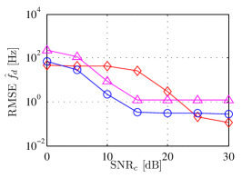
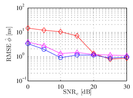
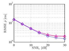
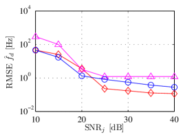
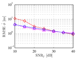
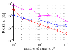
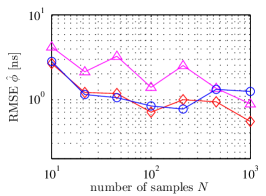
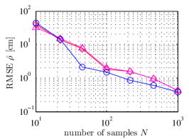
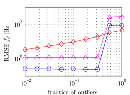
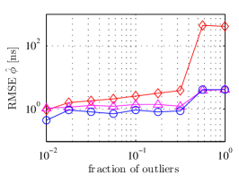
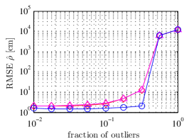
Figure 6: Simulation results, averaged over 1000 Monte Carlo iterations. (a)-(c) varying SNR_c, with SNR${}_{j}=40$ dB. (d)-(f) varying SNR_j, with SNR${}_{c}=30$ dB. (g)-(i) varying the number of samples $N$, with SNR${}_{j}=$ SNR${}_{c}=40$ dB. (j)-(l) in the presence of outliers, varying the fraction of randomly-inserted outliers, with SNR${}_{j}=$ SNR${}_{c}=40$ dB.

IV-B Simulation Results

A complete characterization of the Monte Carlo simulation results is provided in Fig. 6. Due to the fixed resolution of the search grid, WLS and PCP exhibit quantization effects, as shown e.g. in the asymptotic constant behavior at high SNR in Fig. 6 a. Potentially, these effects can be overcome by refining estimates using standard interpolation, zero padding, or adaptive grid search methods. However, their performance is still satisfactory. In fact, all considered estimators are able to obtain accuracy of the order of $1$ Hz or better, when SNR_c and SNR_j are greater than $20$ dB.

Furthermore, we studied the behavior of the proposed methods as the number of samples $N$ varies. The simulation results are shown in Fig. 6 g - 6 i. The proposed WLS estimator shows improved accuracy in small-sample conditions with respect to ULS and PCP, which is advantageous in scenarios with slowly time-varying parameters. The performance of ULS at high SNR and for large $N$ is generally better than PCP and WLS, as shown in Fig. 6 a, d, and g. This is consistent with the expected behavior. As noise vanishes, in fact, the unwrapping procedure results in a linear trend, which can be estimated statistically efficiently by the linear least-squares method.

Finally, in order to analyze the effect of outliers, we performed a set of Monte Carlo simulations substituting a fraction of the data with outliers, uniformly distributed in the $\left[3.5\cdot 10^{-6}\,,4.9\cdot 10^{-6}\right]$ s interval. The outliers are inserted at randomly-selected locations, yielding the results in Fig. 6 j - 6 l. The proposed WLS estimator has considerably improved robustness with respect to the other considered methods. Moreover, it exhibits a threshold behavior, reaching a breakdown point when the fraction of outliers is approximately equal to $40\%$. On the other hand, ULS shows a degraded performance even at a low fraction of outliers, in Fig. 6 g and 6 h, therefore validating the proposed WLS approach. PCP operates first in the frequency domain which gives it a degree of insensitivity to outliers.

IV-C Figure of Merit

The numerical results in Fig. 6 show that, using the considered RTT clock measurement mechanism and the proposed WLS estimator, 100 samples are sufficient to achieve an estimation accuracy of Hertz-order for clock frequency difference, nano-second order for initial phase difference and decimeter-order for ranging in practical noisy and outlier-prone conditions. This can be verified from the curves in Fig. 6 (g)-(i), where an SNR${}_{c}=$SNR${}_{j}=40$ dB is considered. Then, from Fig. 6 (a)-(f) it is possible to observe that such accuracy level is still achieved for SNR_c as low as $10$ dB and SNR_j as low as $20$ dB. More importantly, this accuracy is achieved by the proposed WLS estimator when up to 30$\%$ of the measured data are outliers, as shown in Fig. 6 (j)-(l). Notice that $N=100$ samples correspond to an observation time of $0.1$ s for the considered update period of $T_{s}=10^{-3}$ s, which we have chosen to be of the same order of magnitude as our practical experimental setup. Such an observation time is feasible for most practical applications of joint wireless synchronization and ranging.

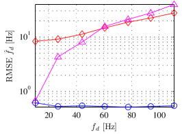
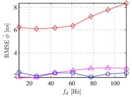
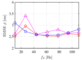
Figure 7: Numerical simulations: RMSE performance of the proposed estimators for different values of the parameter $f_{d}$. Here, SNR${}_{c}=20$ dB, SNR${}_{j}=20$ dB, $N=200$, and no outliers are present. Results are obtained by averaging over 1000 Monte Carlo iterations.

IV-D Sensitivity to Parameter Variations

To evaluate the performance of the considered estimators when the parameter $f_{d}$ varies, we provide the simulation results in Fig. 7, showing that WLS is insensitive to the value of $f_{d}$. On the other hand, ULS and PCP show considerable degradation of the frequency difference estimation performance as $f_{d}$ increases, see Fig. 7(a). As far as the range is concerned, we note that the model in (7) is linear in the range $\rho$, thus it is expected from the theory that the behavior does not change significantly for different values of $\rho$. This is confirmed numerically in Fig. 7(c), where the observed performance is approximately constant.

V Experimental Results

We applied the proposed estimators to experimental data obtained from an in-house test-bed which is based on the IR-UWB technology [18]. In the following, we provide a description of the experimental setup, we evaluate the performance of the considered estimators (ULS, PCP, WLS) on measured data, and eventually we discuss the validation of the proposed model in (7).

V-A Experimental Setup

Experimental setup is shown in Fig. 8. Each of the two nodes was running on its own clock which was provided by a local oscillator in the ML505 evaluation board using a Xilinx Virtex-5 FPGA [40]. Since the two local oscillators were not synchronized, a non-zero frequency difference between the two oscillators was present. In the experimental setup, the master node was programmed to repeat the RTT measurement procedure with a fixed sampling rate of $5$ kHz, and then transfer each result from the TDC to the host computer, where it was stored and used for offline processing. The apparatus and components used in the experiments are relatively low cost and easily available. This brings the proposed idea closer to practice.

As can be seen from Fig. 8, while capturing measurements, we capture ground-truth values of the parameters. The ground-truth values are used for analyzing RMSE of the estimates over measured data. The ground truth of range ($\rho$) is measured using a handheld laser distance meter [41]. Ground-truth values of master and slave clock frequencies ($f_{m},f_{s}$) are captured using Agilent 53230A frequency counter [42]. Ground-truth of phase ($\phi$) is obtained by capturing the clock state using primitive delays in FPGA. The clock of slave node is propagated through these delays and the received first Ping in a sequence Pings from master triggers capture of the clock phase [43].

We placed the master and slave nodes on two carts in line-of-sight conditions in the office-like indoor environment depicted in Fig. 9. For each considered distance a record of 65356 RTT measurement values was acquired. In the experimental conditions, we observed an SNR_c varying from approximately $14$ dB at a distance of $0.5$ m to approximately $0$ dB at the maximum operating distance of about $4$ m. Furthtermore, the SNR_j is approximately $40$ dB, and the fraction of outliers varies from about 5$\%$ up to approximately 20$\%$.

The amplitude of the observed sawtooth waveform is approximately $10$ ns as can be seen in Fig. 5, which is consistent with the nominal clock frequency of $100$ MHz of the FPGA boards used. Furthermore, the period is approximately 30 samples which, considering the sampling frequency of $5$ kHz, corresponds to a frequency difference in the order of $200$ Hz. Such a difference is consistent with the tolerance specification of the local oscillators used in the experiments.

The raw RTT data from the experimental measurement platform was directly used as the input for the WLS estimation algorithm. Whereas, the raw data was pre-processed by a coarse outlier-rejection method before being input into the ULS and PCP algorithms. In particular, the pre-processing outlier rejection method consists of the identification of the outliers by means of the same criterion in (14), and in the following substitution rule: if the outlier is isolated, namely the preceding and following samples are not outliers, then a linear interpolation is performed. Specifically, the outlier sample is replaced by the average of the following and preceding sample. Conversely, if the outlier is not isolated, i.e. if the preceding or following samples are also outliers, the outlier sample is replaced by the median of the entire record.

For validation purposes, we also performed a characterization of ULS and PCP without using the pre-processing step. Results of such characterization, not presented here for brevity, show a considerable performance degradation of one order of magnitude or more with respect to WLS.

Therefore, in the following subsections, we provide results from experimental tests where the pre-processing method is applied to ULS and PCP.

V-B Frequency Difference Experimental Results

We acquired RTT data from the system at four master-slave distances from $1$ m to $4$ m at $1$ m steps. Simultaneously, the related ground-truth data, i.e. the true master-slave clock frequency difference, was acquired using the setup above and found to be approximately $-30$ Hz with small variations among datasets at different distances.

Subsequently, the acquired data was segmented into records, each consisting of 1000 consecutive samples. Each record was processed using the three considered methods. The resulting estimates were compared with the ground-truth, to obtain the results shown in Fig. 11. The proposed WLS method outperforms both the other considered methods, and its performance is relatively insensitive to variations in range. Moreover, the global RMSE, computed taking into account data acquired at all distances, is equal to $0.96$ Hz for the proposed WLS estimator. Thus, the capability of sub-Hertz relative frequency measurement in experimental conditions is demonstrated.

Furthermore, a data record illustrating the presence of outliers is shown in Fig. 10. The presence of outliers can be explained by analyzing the behavior of the receiver employed. In our experimental setup, in fact, the energy-detection receiver cannot distinguish between a proper response signal and an external RF interference signal. Therefore, when external interference bursts cross the pre-defined threshold in the energy detector, they cause spurious detections. Furthermore, the wideband noise which is inherently present in UWB systems can also cause spurious detections. Such spurious detections cause outliers during the RTT measurement procedure.

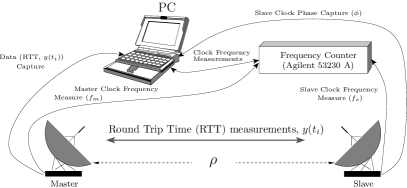
Figure 8: Diagram of the experimental setup.

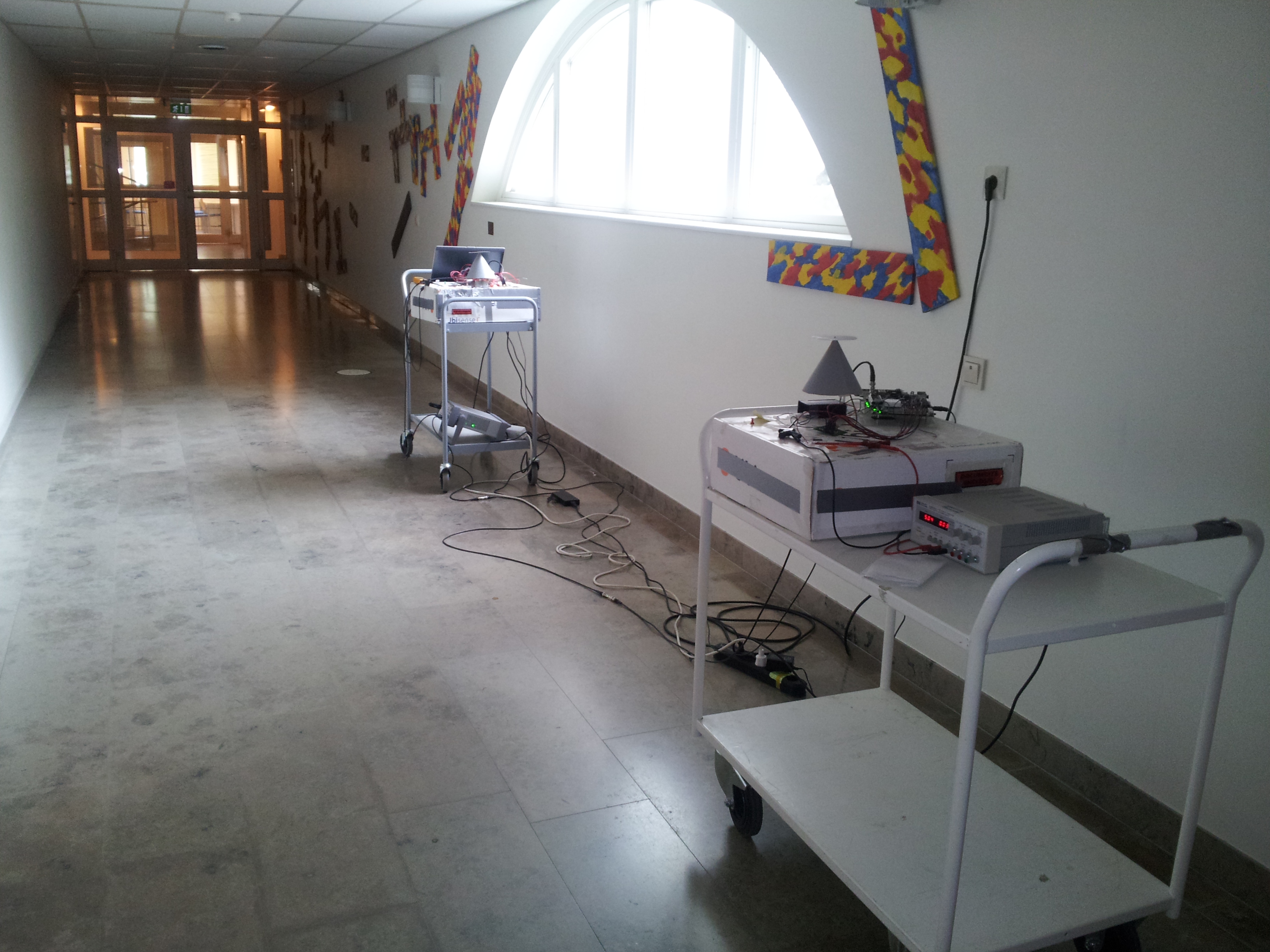
Figure 9: Picture of the experimental setup.

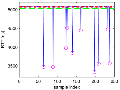
Figure 10: Experimental data record showing outliers denoted with magenta circular markers. The data was obtained with the master and slave antennas placed 5 m apart. The dashed green line denotes the sample mean, which is clearly influenced by the outliers, and the dotted red line denotes the sample median which is robust against outliers.

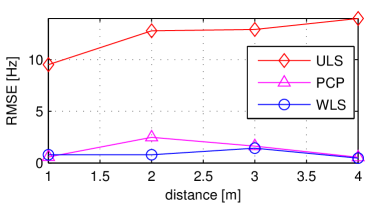
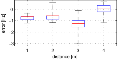
Figure 11: Experimental results for the estimation of frequency difference. (a) RMSE of the frequency difference estimates vs range, for the three considered methods. (b) box plot of the frequency deviation estimation error vs range, for the proposed WLS estimator. The blue edges of each box denote the 25th and 75th percentiles, the central red mark denotes the median, and the top and bottom ends of the black dashed lines denote the maximum and minimum values, respectively.

V-C Phase Experimental Results

Figure 12 shows error between measured phase and estimated phase for various estimators. Since the phase parameter is same for one set of measurements, computing RMSE of phase estimate would require many set of measurements which is practically difficult and time consuming. Hence, instead of RMSE plots, a few phase error estimates are shown in the figure. As can be seen, the phase estimation error is of the order of $1$ ns for WLS and PCP estimators. As expected from simulation results, phase estimation error of ULS is very large.

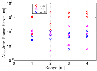
Figure 12: Phase error measurements.

V-D Range Experimental Results

In order to relate the measured RTT to the master-slave range, we performed a calibration procedure based on that described in detail in [18]. The calibration procedure removes various systematic delays, particularly delay in RF front end of the transceivers. In particular, 1000 RTT samples were acquired at a set of known distances from $0.5$ m to $4.5$ m at $0.5$ m steps. Then, the calibration curve was calculated by applying a fifth-order polynomial fitting to the experimental data. The range estimate characterization was then performed on an independent dataset, acquired at four distances from $1$ m to $4$ m at $1$ m steps. We denote the latter dataset as the validation dataset. For each distance in the validation dataset, we acquired multiple 1000-sample records and processed each record using all the considered methods. The range estimation results are summarized in Fig. 13. As clearly noticeable from Fig. 13a, the difference between the three considered estimation methods is less than $1$ cm and, therefore, negligible. The resulting global RMSE, which is calculated over the entire validation dataset, is $17$  cm for the proposed WLS method.

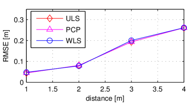
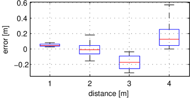
Figure 13: Experimental results for the estimation of range. (a) RMSE of the range estimation error vs actual range, for the three considered methods. (b) box plot of the range estimation error vs actual range, for the proposed WLS estimator. The blue edges of each box denote the 25th and 75th percentiles, the central red mark denotes the median, and the top and bottom ends of the black dashed lines denote the maximum and minimum values, respectively.

V-E Residual Analysis

Figure 14 shows the estimated autocorrelation function over the residuals of the WLS estimator. The residuals are obtained after subtracting noiseless signal template as in (7) using WLS estimates from the measured data at $4$ m. The procedure of analyzing residuals is similar to as discussed in [44]. Fig. 14 also plots the $99\%$ confidence bounds for a white noise sequence. As can be seen, virtually all ACF points fall within these bounds except at the zero lag which thus validates the model proposed in (7).

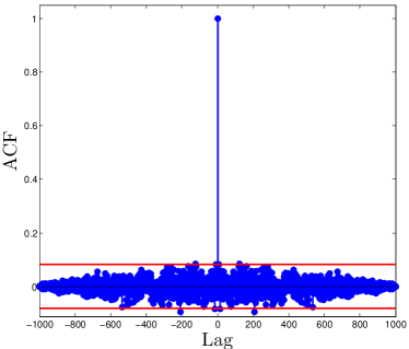
Figure 14: Autocorrelation function over the residuals of WLS, with 99% confidence interval of a white noise sequence. Measurements at $4$ m.

VI Conclusion

In this paper we have proposed a new method to generate wireless measurements for joint clock parameter estimation and range estimation between the clocks of two nodes. We have formulated a mathematical model which captures the measurement generating phenomena. Further, we have developed two robust estimators (PCP and WLS) with different complexities and have compared their performance with the popular ULS estimator. The estimators were compared by simulations using the proposed model. We suggested outlier rejection techniques to handle real-world measurements and compared the estimator performances using data generated by a UWB testbed, reporting favorable experimental RMSE.

We envision that this method has a two-fold use: firstly as a building-block in positioning systems which require wireless node-to-node synchronization. Secondly, this method will give rise to applications where accurate wireless clock synchronization would be beneficial, such as in the internet-of-things, and the machine-to-machine communication frameworks.

To derive the WLS estimator in the efficient form of (11), we first define the matrix

$$\begin{split}\boldsymbol{\Pi}\triangleq\mathbf{1}(\mathbf{1}^{\top}\mathbf{W}\mathbf{1})^{-1}\mathbf{1}^{\top}\mathbf{W}=\frac{\mathbf{1}\mathbf{w}^{\top}}{\mathbf{1}^{\top}\mathbf{w}},\end{split}$$

where the equality follows from $\mathbf{W}\mathbf{1}=\mathbf{w}$. Next, recall that $\mathbf{r}(f_{d},\phi)=\mathbf{y}-h(f_{d},\phi,\mathbf{0})-\delta_{0}\mathbf{1}$. Inserting (10) back into (9), yields a concentrated cost function which we can re-write:

$$\begin{split}J(f_{d},\phi,\hat{\rho})&=\|\mathbf{r}-\boldsymbol{\Pi}\mathbf{r}\|^{2}_{\mathbf{W}}\\ &=\mathbf{r}^{\top}\mathbf{W}\mathbf{r}-2\mathbf{r}^{\top}\mathbf{W}\boldsymbol{\Pi}\mathbf{r}+\mathbf{r}^{\top}\boldsymbol{\Pi}^{\top}\mathbf{W}\boldsymbol{\Pi}\mathbf{r}\\ &=\mathbf{r}^{\top}\mathbf{W}\mathbf{r}-\mathbf{r}^{\top}\mathbf{W}\boldsymbol{\Pi}\mathbf{r}\\ &=\|\mathbf{W}^{1/2}\mathbf{r}\|^{2}_{2}-\frac{\mathbf{r}^{\top}\mathbf{W}\mathbf{1}\mathbf{w}^{\top}\mathbf{r}}{\mathbf{1}^{\top}\mathbf{w}}\\ &=\|\mathbf{w}^{1/2}\odot\mathbf{r}\|^{2}_{2}-\frac{|\mathbf{w}^{\top}\mathbf{r}|^{2}}{\mathbf{1}^{\top}\mathbf{w}},\end{split}$$

using the fact that $\boldsymbol{\Pi}^{\top}\mathbf{W}\boldsymbol{\Pi}=\mathbf{W}\boldsymbol{\Pi}$, thus reproducing (11).

References

- [1] J. Gubbi, R. Buyya, S. Marusic, and M. Palaniswami, “Internet of things (IoT): A vision, architectural elements, and future directions,” Future Generation Computer Systems, vol. 29, no. 7, pp. 1645–1660, 2013.
- [2] S.-Y. Lien, K.-C. Chen, and Y. Lin, “Toward ubiquitous massive accesses in 3gpp machine-to-machine communications,” Communications Magazine, IEEE, vol. 49, pp. 66–74, April 2011.
- [3] Z. Fadlullah, M. Fouda, N. Kato, A. Takeuchi, N. Iwasaki, and Y. Nozaki, “Toward intelligent machine-to-machine communications in smart grid,” Communications Magazine, IEEE, vol. 49, pp. 60–65, April 2011.
- [4] Ubisense, “Ubisense RTLS system.” http://www.ubisense.net/en/, 2014.
- [5] J. Zheng and Y.-C. Wu, “Joint time synchronization and localization of an unknown node in wireless sensor networks,” Signal Processing, IEEE Transactions on, vol. 58, pp. 1309–1320, March 2010.
- [6] B. Denis, J.-B. Pierrot, and C. Abou-Rjeily, “Joint distributed synchronization and positioning in UWB ad hoc networks using toa,” Microwave Theory and Techniques, IEEE Transactions on, vol. 54, pp. 1896–1911, June 2006.
- [7] M. Gholami, S. Gezici, and E. Strom, “TDOA based positioning in the presence of unknown clock skew,” Communications, IEEE Transactions on, vol. 61, pp. 2522–2534, June 2013.
- [8] S. Chepuri, G. Leus, and A. van der Veen, “Joint localization and clock synchronization for wireless sensor networks,” in Signals, Systems and Computers (ASILOMAR), 2012 Conference Record of the Forty Sixth Asilomar Conference on, pp. 1432–1436, Nov 2012.
- [9] S. Chepuri, R. Rajan, G. Leus, and A.-J. van der Veen, “Joint clock synchronization and ranging: Asymmetrical time-stamping and passive listening,” Signal Processing Letters, IEEE, vol. 20, pp. 51–54, Jan 2013.
- [10] B. Etzlinger, F. Meyer, H. Wymeersch, F. Hlawatsch, G. Muller, and A. Springer, “Cooperative simultaneous localization and synchronization: Toward a low-cost hardware implementation,” in Sensor Array and Multichannel Signal Processing Workshop (SAM), 2014 IEEE 8th, pp. 33–36, June 2014.
- [11] P. Carroll, K. Mahmood, S. Zhou, H. Zhou, X. Xu, and J.-H. Cui, “On-demand asynchronous localization for underwater sensor networks,” Signal Processing, IEEE Transactions on, vol. 62, pp. 3337–3348, July 2014.
- [12] H. Wymeersch, J. Lien, and M. Win, “Cooperative localization in wireless networks,” Proceedings of the IEEE, vol. 97, pp. 427–450, Feb 2009.
- [13] S. Gezici, Z. Tian, G. Giannakis, H. Kobayashi, A. Molisch, H. Poor, and Z. Sahinoglu, “Localization via ultra-wideband radios: a look at positioning aspects for future sensor networks,” Signal Processing Magazine, IEEE, vol. 22, pp. 70–84, July 2005.
- [14] S. Dwivedi, D. Zachariah, A. De Angelis, and P. Händel, “Cooperative decentralized localization using scheduled wireless transmissions,” Communications Letters, IEEE, vol. 17, pp. 1240–1243, June 2013.
- [15] D. Mills, “Internet time synchronization: the network time protocol,” Communications, IEEE Transactions on, vol. 39, pp. 1482–1493, Oct 1991.
- [16] S. Ganeriwal, R. Kumar, and M. B. Srivastava, “Timing-sync protocol for sensor networks,” in Proceedings of the 1st international conference on Embedded networked sensor systems, pp. 138–149, ACM, 2003.
- [17] J. Elson, L. Girod, and D. Estrin, “Fine-grained network time synchronization using reference broadcasts,” ACM SIGOPS Operating Systems Review, vol. 36, no. SI, pp. 147–163, 2002.
- [18] A. De Angelis, S. Dwivedi, and P. Händel, “Characterization of a flexible UWB sensor for indoor localization,” IEEE Trans. Instrum. Meas., vol. 62, pp. 905–913, may 2013.
- [19] C.-C. Chui and R. Scholtz, “Time transfer in impulse radio networks,” Communications, IEEE Transactions on, vol. 57, pp. 2771–2781, September 2009.
- [20] P. Carbone, A. Cazzorla, P. Ferrari, A. Flammini, A. Moschitta, S. Rinaldi, T. Sauter, and E. Sisinni, “Low complexity UWB radios for precise wireless sensor network synchronization,” Instrumentation and Measurement, IEEE Transactions on, vol. 62, pp. 2538–2548, Sept 2013.
- [21] Y.-C. Wu, Q. Chaudhari, and E. Serpedin, “Clock synchronization of wireless sensor networks,” Signal Processing Magazine, IEEE, vol. 28, pp. 124–138, Jan 2011.
- [22] B. Etzlinger, H. Wymeersch, and A. Springer, “Cooperative synchronization in wireless networks,” Signal Processing, IEEE Transactions on, vol. 62, pp. 2837–2849, June 2014.
- [23] N. Freris, S. Graham, and P. Kumar, “Fundamental limits on synchronizing clocks over networks,” Automatic Control, IEEE Transactions on, vol. 56, pp. 1352–1364, June 2011.
- [24] I. Skog and P. Händel, “Synchronization by two-way message exchanges: Cramér-rao bounds, approximate maximum likelihood, and offshore submarine positioning,” Signal Processing, IEEE Transactions on, vol. 58, pp. 2351–2362, April 2010.
- [25] D. Zachariah, A. De Angelis, S. Dwivedi, and P. Händel, “Self-localization of asynchronous wireless nodes with parameter uncertainties,” Signal Processing Letters, IEEE, vol. 20, pp. 551–554, June 2013.
- [26] D. Zachariah, A. Angelis, S. Dwivedi, and P. Händel, “Schedule-based sequential localization in asynchronous wireless networks,” EURASIP Journal on Advances in Signal Processing, vol. 2014, no. 1, 2014.
- [27] Y. Shang, W. Ruml, Y. Zhang, and M. P. Fromherz, “Localization from mere connectivity,” in Proceedings of the 4th ACM international symposium on Mobile ad hoc networking & computing, pp. 201–212, ACM, 2003.
- [28] A. Conti, M. Guerra, D. Dardari, N. Decarli, and M. Win, “Network experimentation for cooperative localization,” Selected Areas in Communications, IEEE Journal on, vol. 30, pp. 467–475, February 2012.
- [29] S. Tretter, “Estimating the frequency of a noisy sinusoid by linear regression (corresp.),” Information Theory, IEEE Transactions on, vol. 31, pp. 832–835, Nov 1985.
- [30] I. Skog and P. Händel, “Time synchronization errors in loosely coupled gps-aided inertial navigation systems,” Intelligent Transportation Systems, IEEE Transactions on, vol. 12, pp. 1014–1023, Dec 2011.
- [31] S. Moon, P. Skelly, and D. Towsley, “Estimation and removal of clock skew from network delay measurements,” in INFOCOM ’99. Eighteenth Annual Joint Conference of the IEEE Computer and Communications Societies. Proceedings. IEEE, vol. 1, pp. 227–234 vol.1, Mar 1999.
- [32] ACAM, “acam - Solutions in Time.” http://www.acam.de/, 2014. [Online; accessed 17-June-2014].
- [33] B. Volker and P. Handel, “Frequency estimation from proper sets of correlations,” Signal Processing, IEEE Transactions on, vol. 50, no. 4, pp. 791–802, 2002.
- [34] Mathworks, “Matlab ’unwrap’ function.” http://www.mathworks.se/help/matlab/ref/unwrap.html, 2014. [Online; accessed 17-June-2014].
- [35] A. Zoubir, V. Koivunen, Y. Chakhchoukh, and M. Muma, “Robust estimation in signal processing: A tutorial-style treatment of fundamental concepts,” Signal Processing Magazine, IEEE, vol. 29, no. 4, pp. 61–80, 2012.
- [36] P. Stoica and R. L. Moses, Spectral analysis of signals. Pearson/Prentice Hall Upper Saddle River, NJ, 2005.
- [37] P. J. Rousseeuw, “Least median of squares regression,” Journal of the American statistical association, vol. 79, no. 388, pp. 871–880, 1984.
- [38] V. J. Hodge and J. Austin, “A survey of outlier detection methodologies,” Artificial Intelligence Review, vol. 22, no. 2, pp. 85–126, 2004.
- [39] T. Neu, “Clock jitter analyzed in the time domain, part 1.” http://www.ti.com/lit/an/slyt379/slyt379.pdf, 2010.
- [40] Xilinx, “Ug347 ml505 evaluation platform, user guide.” http://www.xilinx.com/support/documentation/boards_and_kits/ug347.pdf, 2011.
- [41] FLUKE, “Laser distance meter.” http://www.fluke.com/fluke/auen/laser-distance-meters/fluke-411d-laser-distance-meter.htm?PID=69331, 2014.
- [42] Agilent, “53230A 350 MHz Universal Frequency Counter/Timer, 12 digits/s, 20 ps.” http://www.home.agilent.com/en/pd-1893420-pn-53230A/350-mhz-universal-frequency-counter-timer-12-digits-s-20-ps?&cc=SE&lc=eng, 2014. [Online; accessed 17-June-2014].
- [43] S. Dwivedi and P. Händel, “Precise clock parameter estimation and ground truth capture for clock error measurements using FPGAs,” in International IEEE Symposium on Precision Clock Synchronization for Measurement, Control and Communication (ISPCS), (Austin, Tx), September 2014.
- [44] MathWorks, “Residual Analysis with Autocorrelation.” http://www.mathworks.se/help/signal/ug/residual-analysis-with-autocorrelation.html, 2014. [Online; accessed 17-June-2014].