On inhomogeneous Strichartz estimates for fractional Schrödinger equations and their applications

Abstract.

In this paper we obtain some new inhomogeneous Strichartz estimates for the fractional Schrödinger equation in the radial case. Then we apply them to the well-posedness theory for the equation $i\partial_{t}u+|\nabla|^{\alpha}u=V(x,t)u$, $1<\alpha<2$, with radial $\dot{H}^{\gamma}$ initial data below $L^{2}$ and radial potentials $V\in L_{t}^{r}L_{x}^{w}$ under the scaling-critical range $\alpha/r+n/w=\alpha$.

1. Introduction

To begin with, let us consider the following Cauchy problem

$$\begin{cases}i\partial_{t}u+|\nabla|^{\alpha}u=F(x,t),\quad 1<\alpha<2,\\ u(x,0)=f(x),\end{cases}$$ (1.1)

associated with the fractional Schrödinger equation

$$i\partial_{t}u+|\nabla|^{\alpha}u=V(x,t)u$$ (1.2)

where $V:\mathbb{R}^{n+1}\rightarrow\mathbb{C}$ is a potential. This equation has recently attracted interest from mathematical physics. This is because fractional quantum mechanics introduced by Laskin [16] is governed by the equation where it is conjectured that physical realizations may be limited to the cases of $1<\alpha<2$. Of course, the case $\alpha=2$ corresponds to the ordinary quantum mechanics.

By Duhamel’s principle, the solution of (1.1) is given by

$$u(x,t)=e^{it|\nabla|^{\alpha}}f(x)-i\int_{0}^{t}e^{i(t-s)|\nabla|^{\alpha}}F(\cdot,s)ds,$$ (1.3)

where the propagator $e^{it|\nabla|^{\alpha}}$ is given by means of the Fourier transform, as follows:

$$e^{it|\nabla|^{\alpha}}f(x)=\frac{1}{(2\pi)^{n}}\int_{\mathbb{R}^{n}}e^{ix\cdot\xi+it|\xi|^{\alpha}}\widehat{f}(\xi)d\xi.$$

Then the standard approach to the problem (1.1) is to obtain the corresponding Strichartz estimates which control space-time integrability of (1.3) in view of that of the initial datum $f$ and the forcing term $F$.

In the classical case $\alpha=2$, the Strichartz estimates originated by Strichartz [23] have been extensively studied by many authors ([9, 14, 2, 12, 8, 24, 15, 17, 18, 5, 6, 20]). Over the past several years, considerable attention has been paid to the fractional order where $1<\alpha<2$ in the radial case (see [21, 11, 13] and references therein). From these works, when $2n/(2n-1)\leq\alpha<2$, the homogeneous Strichartz estimate

$$\|e^{it|\nabla|^{\alpha}}f\|_{L^{q}_{t}L^{p}_{x}}\lesssim\|f\|_{\dot{H}^{\gamma}}$$ (1.4)

holds for radial functions $f\in\dot{H}^{\gamma}(\mathbb{R}^{n})$ if

$$\frac{\alpha}{q}+\frac{n}{p}=\frac{n}{2}-\gamma,\quad 2\leq q\leq\infty\quad\mbox{and}\quad(q,p)\neq(2,\frac{4n-2}{2n-3}).$$ (1.5)

Here the condition (1.5) is optimal if $2n/(2n-1)<\alpha<2$. But when $\alpha=2n/(2n-1)$, (1.4) is unknown for the endpoint $(q,p)=(2,(4n-2)/(2n-3))$. Also, it is known that the estimate does not hold in general if $f$ does not have radial symmetry.

Now, by duality and the Christ-Kiselev lemma ([4]), one may use (1.4) with $\gamma=0$ to get some inhomogeneous estimates

$$\Big{\|}\int_{0}^{t}e^{i(t-s)|\nabla|^{\alpha}}F(\cdot,s)ds\Big{\|}_{L^{q}_{t}L^{p}_{x}}\lesssim\|F\|_{L^{\widetilde{q}^{\prime}}_{t}L^{\widetilde{p}^{\prime}}_{x}}$$ (1.6)

for $(q,p)$ and $(\widetilde{q},\widetilde{p})$ which satisfy (1.5) with $\gamma=0$ and $q>\widetilde{q}^{\prime}$. This means that $(q,p)$ and $(\widetilde{q},\widetilde{p})$ lie on the segment $AD$ in Figure 1. However, these trivial estimates are not enough to imply the well-posedness for the equation (1.2) with the initial data $f\in\dot{H}^{\gamma}(\mathbb{R}^{n})$ beyond the case $\gamma=0$. When $\gamma\neq 0$ we need to obtain (1.6) on a wider range of $(q,p)$ and $(\widetilde{q},\widetilde{p})$. See Section 2 for details.

Let us first mention the following necessary conditions for (1.6):

$$\alpha(\frac{1}{q}+\frac{1}{\widetilde{q}})-n(1-\frac{1}{p}-\frac{1}{\widetilde{p}})=0$$ (1.7)

and

$$\frac{1}{q}+\frac{n}{p}<\frac{n}{2},\quad\frac{1}{\widetilde{q}}+\frac{n}{\widetilde{p}}<\frac{n}{2}.$$ (1.8)

The first is just the scaling condition and the second will be shown in Section 4.

Our main result in this paper is the following theorem where we obtain (1.6) on the open segment $BC$ in Figure 1.

Theorem 1.1.

Let $n\geq 2$ and $2n/(2n-1)\leq\alpha<2$. Assume that $F(x,t)$ is a radial function with respect to the spatial variable $x$. Then we have

$$\Big{\|}\int_{0}^{t}e^{i(t-s)|\nabla|^{\alpha}}F(\cdot,s)ds\Big{\|}_{L^{q}_{x,t}}\lesssim\|F\|_{L^{\widetilde{q}^{\prime}}_{x,t}}$$ (1.9)

if

$$\frac{1}{q},\frac{1}{\widetilde{q}}<\frac{n}{2(n+1)}\quad\mbox{and}\quad\frac{1}{q}+\frac{1}{\widetilde{q}}=\frac{n}{n+\alpha}.$$ (1.10)

Remark 1.2.

It should be noted that the range (1.10) is sharp. Namely, the second condition in (1.10) is the scaling condition for (1.9) (see (1.7)), and the first one is the necessary condition (1.8) when $q=p$ and $\widetilde{q}=\widetilde{p}$.

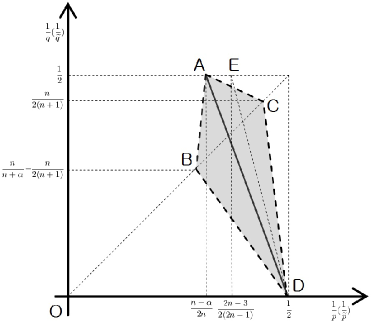
Figure 1. The range for Corollary 1.3. Here the open segment $(B,C)$ is the range for (1.9), and $[A,D]$ is the range for (1.6).

From interpolation between (1.6) and (1.9), we can directly obtain further estimates when $(q,p)$ and $(\widetilde{q},\widetilde{p})$ are contained in the open quadrangle with vertices $A,B,D,C$. Precisely, we have the following corollary.

Corollary 1.3.

Let $n\geq 2$ and $2n/(2n-1)\leq\alpha<2$. Assume that $F(x,t)$ is a radial function with respect to the spatial variable $x$, and that $(q,p)$ and $(\widetilde{q},\widetilde{p})$ satisfy the necessary conditions (1.7) and (1.8). Then we have

$$\Big{\|}\int_{0}^{t}e^{i(t-s)|\nabla|^{\alpha}}F(\cdot,s)ds\Big{\|}_{L^{q}_{t}L^{p}_{x}}\lesssim\|F\|_{L^{\widetilde{q}^{\prime}}_{t}L^{\widetilde{p}^{\prime}}_{x}}$$ (1.11)

if the following conditions hold:

• For $(q,p)$,

  $$\frac{-n(n+2-\alpha)}{(2\alpha-1)n+\alpha}(\frac{1}{p}-\frac{1}{2})<\frac{1}{q}<\frac{-n}{(\alpha-1)n+\alpha}(\frac{1}{p}-\frac{n-\alpha}{2n})+\frac{1}{2},$$ (1.12)

  and

  $$\frac{1}{p}>\frac{(\alpha-1)n^{2}-\alpha^{2}n-\alpha^{2}}{((2\alpha-1)n+\alpha)n}\frac{1}{q}+\frac{\alpha(n+2-\alpha)}{2((2\alpha-1)n+\alpha)}.$$ (1.13)

• Similarly for $(\widetilde{q},\widetilde{p})$.

Let us give more details about the conditions in the above corollary. The line $BD$ in Figure 1 is when the equality holds in the first inequality of (1.12). Similarly, the lines $AC$ and $AB$ correspond to the second inequality in (1.12) and the inequality (1.13), respectively. Finally, the line $CD$ is sharp because it is determined from the necessary condition (1.8).

Now we apply the above Strichartz estimates to the well-posedness theory for the fractional Schrödinger equation in the radial case:

$$\begin{cases}i\partial_{t}u+|\nabla|^{\alpha}u=V(x,t)u,\quad 1<\alpha<2,\\ u(x,0)=f(x),\end{cases}$$ (1.14)

where we assume that $u$, $f$ and $V$ are radial functions with respect to the spatial variable $x$. We obtain the following well-posedness for (1.14) with $\dot{H}^{\gamma}$ initial data $f$ below $L^{2}$ and potentials $V\in L_{t}^{r}L_{x}^{w}$ under the scaling-critical range $\alpha/r+n/w=\alpha$. The Cauchy problem (1.14) was studied in [7, 19] particularly when $\alpha=2$ and $\gamma=0$.

Theorem 1.4.

Let $\frac{2n}{2n-1}\leq\alpha<2$ and $\frac{-(\alpha-1)n}{2(n+1)}<\gamma\leq 0$ for $n\geq 2$. Assume that $f\in\dot{H}^{\gamma}(\mathbb{R}^{n})$ and $V\in L_{t}^{r}([0,T];L_{x}^{w}(\mathbb{R}^{n}))$ for some $T>0$. Then there exists a unique solution $u\in C([0,T];\dot{H}^{\gamma}(\mathbb{R}^{n}))\cap L_{t}^{q}([0,T];L_{x}^{p}(\mathbb{R}^{n}))$ of (1.14) if

$$\frac{\alpha}{q}+\frac{n}{p}=\frac{n}{2}-\gamma,\quad\frac{\alpha}{r}+\frac{n}{w}=\alpha,$$ (1.15)

$$\frac{-\gamma}{\alpha-1}<\frac{1}{q}<\frac{\gamma}{(\alpha-1)n}+\frac{1}{2},$$ (1.16)

and

$$1-\frac{1}{q}-\frac{n(n+\alpha)(\alpha-1)+2\gamma((2\alpha-1)n+\alpha)}{2n(n+\alpha)(\alpha-1)}<\frac{1}{r}<1-\frac{1}{q}+\frac{\gamma(n+2-\alpha)}{(n+\alpha)(\alpha-1)}.$$ (1.17)

Remark 1.5.

The condition $\alpha/r+n/w=\alpha$ on the potential is critical in the sense of scaling. Indeed, $u_{\epsilon}(x,t)=u(\epsilon x,\epsilon^{\alpha}t)$ takes (1.14) into $i\partial_{t}u_{\epsilon}+|\nabla|^{\alpha}u_{\epsilon}=V_{\epsilon}(x,t)u_{\epsilon}$ with $V_{\epsilon}(x,t)=\epsilon^{\alpha}V(\epsilon x,\epsilon^{\alpha}t)$. Hence the norm

$$\|V_{\epsilon}\|_{L_{t}^{r}L_{x}^{w}}=\|V_{\epsilon}\|_{L_{t}^{r}(\mathbb{R};L_{x}^{w}(\mathbb{R}^{n}))}=\epsilon^{\alpha-\alpha/r-n/w}\|V\|_{L_{t}^{r}L_{x}^{w}}$$

is independent of $\epsilon$ precisely when $\alpha/r+n/w=\alpha$.

Remark 1.6.

In Proposition 3.9 of [11], the inhomogeneous estimates were shown in certain region that lies below the segment $ED$ in Figure 1. (Note that $(1/q,1/p)\in ED$ if and only if $q,p\geq 2$ and $2/q+(2n-1)/p=n-1/2$. Also, the point $E$ is the same as $A$ when $\alpha=2n/(2n-1)$.) By interpolation between these and our estimates, we can also obtain further estimates in the triangle with vertices $A,C,E$. We omit the details since it does not affect the range $\frac{-(\alpha-1)n}{2(n+1)}<\gamma\leq 0$ of $\gamma$ in Theorem 1.4 (see Section 2).

The rest of the paper is organized as follows. In Section 2, we prove Theorem 1.4 by making use of the Strichartz estimates (1.4) and (1.11). Section 3 is devoted to proving Theorem 1.1, and in Section 4 we show the necessary condition (1.8). In the final section, Section 5, we show Lemma 3.5 which gives some estimates for Bessel functions and is used for the proof of Theorem 1.1.

Throughout the paper, we shall use the letter $C$ to denote positive constants which may be different at each occurrence. We also use the symbol $\widehat{f}$ to denote the Fourier transform of $f$, and denote $A\lesssim B$ and $A\sim B$ to mean $A\leq CB$ and $CB\leq A\leq CB$, respectively, with unspecified constants $C>0$.

2. Application

In this section we prove Theorem 1.4. The proof is quite standard but we need to observe that if $(q,p)$ and $(\widetilde{q},\widetilde{p})$ satisfy the inhomogeneous estimate (1.11), then the midpoint of them lies on the segment $AD$. Note that $(1/q,1/p)\in AD$ if and only if $q,p\geq 2$ and $\alpha/q+n/p=n/2$. Hence, if $\alpha/q+n/p=n/2-\gamma$ for $\gamma\in\mathbb{R}$, then $(\widetilde{q},\widetilde{p})$ should satisfy $\alpha/\widetilde{q}+n/\widetilde{p}=n/2+\gamma$ to give (1.11). In what follows, it will be convenient to keep in mind this key observation.

By Duhamel’s principle, the solution of (1.14) is given by

$$\Phi(u):=e^{it|\nabla|^{\alpha}}f(x)-i\int_{0}^{t}e^{i(t-s)|\nabla|^{\alpha}}V(\cdot,s)u(\cdot,s)ds.$$ (2.1)

Then the standard fixed-point argument is to choose the solution space on which $\Phi$ is a contraction mapping. The Strichartz estimates play a central role in this step. Indeed, by the estimates (1.4) and (1.11), we see that

$$\|\Phi(u)\|_{L_{t}^{q}([0,T];L_{x}^{p})}\leq C\|f\|_{\dot{H}^{\gamma}}+C\|Vu\|_{L^{\widetilde{q}^{\prime}}_{t}([0,T];L^{\widetilde{p}^{\prime}}_{x})}$$ (2.2)

if

$$\frac{-(\alpha-1)n}{2(n+1)}<\gamma\leq 0$$ (2.3)

$$\frac{\alpha}{q}+\frac{n}{p}=\frac{n}{2}-\gamma,\quad\frac{\alpha}{\widetilde{q}}+\frac{n}{\widetilde{p}}=\frac{n}{2}+\gamma,$$ (2.4)

$$\frac{-\gamma}{\alpha-1}<\frac{1}{q}<\frac{\gamma}{(\alpha-1)n}+\frac{1}{2},$$ (2.5)

and

$$\frac{\gamma(n+2-\alpha)}{(n+\alpha)(\alpha-1)}<\frac{1}{\widetilde{q}}<\frac{n(n+\alpha)(\alpha-1)+2\gamma((2\alpha-1)n+\alpha)}{2n(n+\alpha)(\alpha-1)}.$$ (2.6)

Here, the conditions (2.3) and (2.5) are given from that the line $\frac{\alpha}{q}+\frac{n}{p}=\frac{n}{2}-\gamma$ lies in the closed triangle with vertices $A,C,D$ except the closed segments $[A,C],[C,D]$. Note that $\gamma=\frac{-(\alpha-1)n}{2(n+1)}$ when this line passes through the point $C$. Similarly, the condition (2.6) is given from that the line $\frac{\alpha}{\widetilde{q}}+\frac{n}{\widetilde{p}}=\frac{n}{2}+\gamma$ lies in the closed triangle with vertices $A,B,D$ except the closed segments $[A,B],[B,D]$.

By Hölder’s inequality, we now get

$$\|\Phi(u)\|_{L_{t}^{q}([0,T];L_{x}^{p})}\leq C\|f\|_{\dot{H}^{\gamma}}+C\|V\|_{L^{r}_{t}([0,T];L^{w}_{x})}\|u\|_{L^{q}_{t}([0,T];L^{p}_{x})}$$

if $\alpha/r+n/w=\alpha$ and the condition (1.17) holds. Indeed, when applying Hölder’s inequality to the second term in the right-hand side of (2.2), the conditions $\alpha/r+n/w=\alpha$ and (1.17) follow from (2.4) and (2.6), respectively.

From the above argument and the linearity, it follows that

$$\|\Phi(u)-\Phi(v)\|_{L_{t}^{q}([0,T];L_{x}^{p})} \leq C\|V\|_{L^{r}_{t}([0,T];L^{w}_{x})}\|u-v\|_{L^{q}_{t}([0,T];L^{p}_{x})}$$

$$\leq\frac{1}{2}\|u-v\|_{L^{q}_{t}([0,T];L^{p}_{x})},$$

which says that $\Phi$ is a contraction mapping, if $T$ is sufficiently small. But here, since the above process works also on time-translated small intervals if $u(\cdot,t)\in\dot{H}^{\gamma}(\mathbb{R}^{n})$ for all $t\geq 0$, the smallness assumption on $T$ can be removed by iterating the process a finite number of times. For this we will show that

$$\|u\|_{L_{t}^{\infty}\dot{H}_{x}^{\gamma}}\lesssim\|f\|_{\dot{H}^{\gamma}}+\|V\|_{L^{r}_{t}L^{w}_{x}}\|u\|_{L^{q}_{t}L^{p}_{x}}.$$ (2.7)

From (2.1), we first see that

$$\|u\|_{L_{t}^{\infty}\dot{H}_{x}^{\gamma}}\lesssim\|e^{it|\nabla|^{\alpha}}D^{\gamma}f\|_{L_{t}^{\infty}L_{x}^{2}}+\Big{\|}\int_{0}^{t}e^{i(t-s)|\nabla|^{\alpha}}D^{\gamma}(V(\cdot,s)u(\cdot,s))ds\Big{\|}_{L_{t}^{\infty}L_{x}^{2}}.$$

Since $e^{it|\nabla|^{\alpha}}$ is an isometry in $L^{2}$, the first term in the right-hand side is clearly bounded by $\|f\|_{\dot{H}^{\gamma}}$. On the other hand, by the inhomogeneous estimate (1.6) the second term is bounded by $\|D^{\gamma}(Vu)\|_{L_{t}^{\widetilde{u}^{\prime}}L_{x}^{\widetilde{v}^{\prime}}}$, where $\widetilde{u},\widetilde{v}\geq 2$ and $\alpha/\widetilde{u}+n/\widetilde{v}=n/2$. Here we use the Sobolev embedding

$$\|g\|_{L^{b}}\lesssim\|D^{\beta}g\|_{L^{a}},$$

where $1/a-1/b=\beta/n$ with $0\leq\beta<n/a$ and $1<a<\infty$, and Hölder’s inequality to get

$$\|D^{\gamma}(Vu)\|_{L_{t}^{\widetilde{u}^{\prime}}L_{x}^{\widetilde{v}^{\prime}}} \lesssim\|Vu\|_{L_{t}^{\widetilde{u}^{\prime}}L_{x}^{a}}$$

$$\leq\|V\|_{L_{t}^{r}L_{x}^{w}}\|u\|_{L_{t}^{q}L_{x}^{p}}.$$

The required conditions here are summarized as follows:

$$\widetilde{u},\widetilde{v}\geq 2,\quad\frac{\alpha}{\widetilde{u}}+\frac{n}{\widetilde{v}}=\frac{n}{2},$$

$$\frac{1}{a}-\frac{1}{\widetilde{v}^{\prime}}=\frac{-\gamma}{n},\quad 0\leq-\gamma<\frac{n}{a},\quad 1<a<\infty,$$

$$\frac{1}{\widetilde{u}^{\prime}}=\frac{1}{r}+\frac{1}{q},\quad\frac{1}{a}=\frac{1}{w}+\frac{1}{p}.$$

But, the inequalities $\widetilde{u},\widetilde{v}\geq 2$ and $1<a<\infty$ are satisfied automatically from the conditions on $q,r,p,w$ in Theorem 1.4. On the other hand, the inequality $0\leq-\gamma<\frac{n}{a}$ is redundant because $\widetilde{v}\geq 2$. The remaining four equalities is reduced to the following one equality

$$\frac{\alpha}{q}+\frac{n}{p}-\frac{n}{2}+\gamma=-(\frac{\alpha}{r}+\frac{n}{w}-\alpha)$$

which is clearly satisfied from the condition (1.15). Consequently, we get (2.7).

3. Inhomogeneous Strichartz estimates

In this section we prove Theorem 1.1. Let us first consider the multiplier operators $P_{k}$ for $k\in\mathbb{Z}$ defined by

$$\widehat{P_{k}f}=\phi(|\cdot|/2^{k})\widehat{f},$$

where $\phi:\mathbb{R}\rightarrow[0,1]$ is a smooth cut-off function which is supported in $(1/2,2)$ and satisfies $\sum_{k\in\mathbb{Z}}\phi(\cdot/2^{k})=1$. Then we will obtain the following frequency localized estimates (Proposition 3.1) which imply Theorem 1.1.

Proposition 3.1.

Let $n\geq 2$ and $2n/(2n-1)\leq\alpha<2$. Assume that $F(x,t)$ is a radial function with respect to the spatial variable $x$. Then we have

$$\Big{\|}\int_{\mathbb{R}}e^{i(t-s)|\nabla|^{\alpha}}P_{k}F(\cdot,s)ds\Big{\|}_{L^{q}_{x,t}}\lesssim\|F\|_{L^{\widetilde{q}^{\prime}}_{x,t}}$$ (3.1)

uniformly in $k\in\mathbb{Z}$ if

$$\frac{1}{q},\frac{1}{\widetilde{q}}<\frac{n}{2(n+1)}\quad\mbox{and}\quad\frac{1}{q}+\frac{1}{\widetilde{q}}=\frac{n}{n+\alpha}.$$ (3.2)

Indeed, since $q>2$ from the first condition in (1.10), by the Littlewood-Paley theorem and Minkowski integral inequality, one can see that

$$\Big{\|}\int_{\mathbb{R}}e^{i(t-s)|\nabla|^{\alpha}}F(\cdot,s)ds\Big{\|}_{L^{q}_{x,t}}^{2} \leq C\Big{\|}\Big{(}\sum_{k\in\mathbb{Z}}\Big{|}\int_{\mathbb{R}}e^{i(t-s)|\nabla|^{\alpha}}P_{k}F(\cdot,s)ds\Big{|}^{2}\Big{)}^{1/2}\Big{\|}_{L^{q}_{x,t}}^{2}$$

$$\leq C\sum_{k\in\mathbb{Z}}\Big{\|}\int_{\mathbb{R}}e^{i(t-s)|\nabla|^{\alpha}}P_{k}\big{(}\sum_{|j-k|\leq 1}P_{j}F(\cdot,s)\big{)}ds\Big{\|}_{L^{q}_{x,t}}^{2}.$$

Now, by (3.1), the right-hand side in the above is bounded by

$$C\sum_{k\in\mathbb{Z}}\big{\|}\sum_{|j-k|\leq 1}P_{j}F\big{\|}_{L^{\widetilde{q}^{\prime}}_{x,t}}^{2}.$$

Since $\widetilde{q}^{\prime}<2$, using the Minkowski integral inequality and Littlewood-Paley theorem, this is bounded by $C\|F\|_{L^{\widetilde{q}^{\prime}}_{x,t}}^{2}$. By this boundedness and $\widetilde{q}^{\prime}<2<q$, one may now use the Christ-Kiselev lemma ([4]) to obtain

$$\Big{\|}\int_{0}^{t}e^{i(t-s)|\nabla|^{\alpha}}F(\cdot,s)ds\Big{\|}_{L^{q}_{x,t}}\lesssim\|F\|_{L^{\widetilde{q}^{\prime}}_{x,t}}$$

as desired.

Now it remains to prove the above proposition.

3.1. Proof of Proposition 3.1

Since we are assuming the scaling condition in (3.2), by rescaling $(x,t)\rightarrow(\lambda x,\lambda^{\alpha}t)$, we may show (3.1) only for $k=0$.

Let us first consider $x=rx^{\prime}$, $y=\lambda y^{\prime}$ and $\xi=\rho\xi^{\prime}$ for $x^{\prime},y^{\prime},\xi^{\prime}\in S^{n-1}$, where $r=|x|$, $\lambda=|y|$ and $\rho=|\xi|$. Then by using the fact (see [22], p. 347) that

$$\int_{S^{n-1}}e^{-ir\rho x^{\prime}\cdot\xi^{\prime}}dx^{\prime}=c_{n}(r\rho)^{-\frac{n-2}{2}}J_{\frac{n-2}{2}}(r\rho),$$

where $J_{m}$ denotes the Bessel function with order $m$, it is easy to see that

$$\int_{\mathbb{R}}e^{i(t-s)|\nabla|^{\alpha}}P_{0}F(\cdot,s)ds$$ (3.3)

$$=\int_{\mathbb{R}}\int_{\mathbb{R}}\int_{\mathbb{R}}\int_{S^{n-1}}\int_{S^{n-1}}e^{i\rho(rx^{\prime}-\lambda y^{\prime})\cdot\xi^{\prime}+i(t-s)\rho^{\alpha}}\phi(\rho)F(\lambda y^{\prime},s)(\lambda\rho)^{n-1}dy^{\prime}d\xi^{\prime}d\rho d\lambda ds$$

$$=r^{-\frac{n-2}{2}}\int_{\mathbb{R}}\lambda^{-\frac{n-2}{2}}\bigg{(}\int_{\mathbb{R}}e^{i(t-s)\rho^{\alpha}}J_{\frac{n-2}{2}}(r\rho)J_{\frac{n-2}{2}}(\lambda\rho)\rho\phi(\rho)d\rho\bigg{)}\big{[}\lambda^{n-1}F(\lambda y^{\prime},s)\big{]}d\lambda ds.$$

Now we define the operators $T_{j}h$, $j\geq 0$, as

$$T_{0}h(r,t)=\chi_{(0,1)}(r)~{}r^{-\frac{n-2}{2}}\int_{0}^{\infty}e^{it\rho^{\alpha}}J_{\frac{n-2}{2}}(r\rho)\varphi(\rho)h(\rho)d\rho$$ (3.4)

and for $j\geq 1$

$$T_{j}h(r,t)=\chi_{[2^{j-1},2^{j})}(r)~{}r^{-\frac{n-2}{2}}\int_{0}^{\infty}e^{it\rho^{\alpha}}J_{\frac{n-2}{2}}(r\rho)\varphi(\rho)h(\rho)d\rho,$$ (3.5)

where $\chi_{A}$ denotes the characteristic function of a set $A$ and $\varphi^{2}(\rho)=\rho\phi(\rho)$. Then the adjoint operator $T^{*}_{k}$ of $T_{k}$ is given by

$$T^{*}_{0}H(\rho)=\varphi(\rho)\int_{\mathbb{R}}e^{-is\rho^{\alpha}}\int_{0}^{\infty}\chi_{(0,1)}(\lambda)~{}\lambda^{-\frac{n-2}{2}}J_{\frac{n-2}{2}}(\lambda\rho)H(\lambda,s)d\lambda ds$$

and for $k\geq 1$

$$T^{*}_{k}H(\rho)=\varphi(\rho)\int_{\mathbb{R}}e^{-is\rho^{\alpha}}\int_{0}^{\infty}\chi_{[2^{k-1},2^{k})}(\lambda)~{}\lambda^{-\frac{n-2}{2}}J_{\frac{n-2}{2}}(\lambda\rho)H(\lambda,s)d\lambda ds.$$ (3.6)

Hence, since $F(\lambda y^{\prime},s)$ is independent of $y^{\prime}\in S^{n-1}$, by setting $H(\lambda,s)=F(\lambda y^{\prime},s)$, it follows from (3.3) that

$$\int_{\mathbb{R}}e^{i(t-s)|\nabla|^{\alpha}}P_{0}F(\cdot,s)ds=\sum_{j,k\geq 0}T_{j}T^{*}_{k}(\lambda^{n-1}H).$$

Now we are reduced to showing that

$$\Big{\|}\sum_{j,k\geq 0}T_{j}T^{*}_{k}(\lambda^{n-1}H)\Big{\|}_{L^{q}_{t}\mathfrak{L}^{q}_{r}}\lesssim\|H\|_{L^{\widetilde{q}^{\prime}}_{t}\mathfrak{L}^{\widetilde{q}^{\prime}}_{r}},$$ (3.7)

where we denote by $\mathfrak{L}^{q}_{r}$ the space $L^{q}(r^{n-1}dr)$.

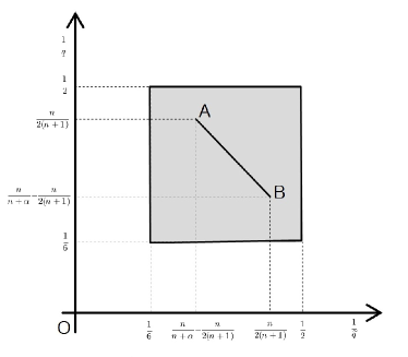
Figure 2. The range of $q,\widetilde{q}$ for Lemma 3.2. Here the open segment $(A,B)$ is the range for Proposition 3.1 (see (3.2)).

From now on, we will show (3.7) by making use of the following lemma which will be obtained in Subsection 3.2.

Lemma 3.2.

Let $n\geq 2$ and $2n/(2n-1)\leq\alpha<2$. Then we have for $j,k\geq 0$

$$\|T_{j}T^{*}_{k} (\lambda^{n-1}H)\|_{L^{q}_{t}\mathfrak{L}^{q}_{r}}$$

$$\lesssim 2^{j(\frac{2n+1}{2q}-\frac{2n-1}{4})}2^{k(\frac{2n+1}{2\widetilde{q}}-\frac{2n-1}{4})}2^{\frac{-|j-k|}{2}(\frac{1}{2}-\max(\frac{1}{q},\frac{1}{\widetilde{q}}))}\|H\|_{L^{\widetilde{q}^{\prime}}_{t}\mathfrak{L}^{\widetilde{q}^{\prime}}_{r}}$$

if $2\leq q,\widetilde{q}\leq 6$ (see Figure 2).

The case $2n/(2n-1)<\alpha<2$. We first decompose the sum over $j,k$ into two parts, $j\leq k$ and $j\geq k$:

$$\sum_{j,k\geq 0} \|T_{j}T^{*}_{k}(\lambda^{n-1}H)\|_{L^{q}_{t}\mathfrak{L}^{q}_{r}}$$

$$\leq\sum_{j=0}^{\infty}\sum_{k=j}^{\infty}\|T_{j}T^{*}_{k}(\lambda^{n-1}H)\|_{L^{q}_{t}\mathfrak{L}^{q}_{r}}+\sum_{k=0}^{\infty}\sum_{j=k}^{\infty}\|T_{j}T^{*}_{k}(\lambda^{n-1}H)\|_{L^{q}_{t}\mathfrak{L}^{q}_{r}}.$$

When $j\leq k$, using Lemma 3.2, we then have

$$\sum_{j=0}^{\infty}\sum_{k=j}^{\infty} \|T_{j}T^{*}_{k}(\lambda^{n-1}H)\|_{L^{q}_{t}\mathfrak{L}^{q}_{r}}$$

$$\lesssim\sum_{j=0}^{\infty}\sum_{k=j}^{\infty}2^{j(\frac{2n+1}{2q}-\frac{2n-1}{4})}2^{k(\frac{2n+1}{2\widetilde{q}}-\frac{2n-1}{4})}2^{\frac{-|j-k|}{2}(\frac{1}{2}-\max(\frac{1}{q},\frac{1}{\widetilde{q}}))}\|H\|_{L^{\widetilde{q}^{\prime}}_{t}\mathfrak{L}^{\widetilde{q}^{\prime}}_{r}}$$

$$=\sum_{j=0}^{\infty}2^{j(\frac{2n+1}{2q}-\frac{2n-2}{4}-\frac{1}{2}\max(\frac{1}{q},\frac{1}{\widetilde{q}}))}\sum_{k=j}^{\infty}2^{k(\frac{2n+1}{2\widetilde{q}}-\frac{n}{2}+\frac{1}{2}\max(\frac{1}{q},\frac{1}{\widetilde{q}}))}\|H\|_{L^{\widetilde{q}^{\prime}}_{t}\mathfrak{L}^{\widetilde{q}^{\prime}}_{r}}.$$

Note here that the first condition in (3.2) implies

$$\frac{2n+1}{2\widetilde{q}}-\frac{n}{2}+\frac{1}{2}\max(\frac{1}{q},\frac{1}{\widetilde{q}})\leq(n+1)\max(\frac{1}{q},\frac{1}{\widetilde{q}})-\frac{n}{2}<0.$$ (3.8)

From this, it follows that

$$\sum_{j=0}^{\infty}2^{j(\frac{2n+1}{2q}-\frac{2n-2}{4}-\frac{1}{2}\max(\frac{1}{q},\frac{1}{\widetilde{q}}))}\sum_{k=j}^{\infty} 2^{k(\frac{2n+1}{2\widetilde{q}}-\frac{n}{2}+\frac{1}{2}\max(\frac{1}{q},\frac{1}{\widetilde{q}}))}$$

$$\lesssim\sum_{j=0}^{\infty}2^{j(\frac{2n+1}{2}(\frac{1}{q}+\frac{1}{\widetilde{q}})-\frac{2n-1}{2})}.$$

On the other hand, the second condition in (3.2) implies

$$\frac{2n+1}{2}(\frac{1}{q}+\frac{1}{\widetilde{q}})-\frac{2n-1}{2}<0$$ (3.9)

since $\alpha>2n/(2n-1)$. Consequently, we get

$$\sum_{j=0}^{\infty}\sum_{k=j}^{\infty}\|T_{j}T^{*}_{k}(\lambda^{n-1}H)\|_{L^{q}_{t}\mathfrak{L}^{q}_{r}} \lesssim\sum_{j=0}^{\infty}2^{j(\frac{2n+1}{2}(\frac{1}{q}+\frac{1}{\widetilde{q}})-\frac{2n-1}{2})}\|H\|_{L^{\widetilde{q}^{\prime}}_{t}\mathfrak{L}^{\widetilde{q}^{\prime}}_{r}}$$

$$\lesssim\|H\|_{L^{\widetilde{q}^{\prime}}_{t}\mathfrak{L}^{\widetilde{q}^{\prime}}_{r}}$$

as desired. The other part where $j\geq k$ follows clearly from the same argument.

The case $\alpha=2n/(2n-1)$. The previous argument is no longer available in this case, since the left-hand side in (3.9) becomes zero. But here we deduce (3.7) from bilinear interpolation between bilinear form estimates which follow from Lemma 3.2. This enables us to gain some summability as before.

Let us first define the bilinear operators $B_{j,k}$ by

$$B_{j,k}(H,\widetilde{H})=\Big{\langle}T^{*}_{k}(\lambda^{n-1}H),T^{*}_{j}(\lambda^{n-1}\widetilde{H})\Big{\rangle}_{L^{2}_{r,t}},$$

where $\langle\,\,,\,\rangle$ denotes the usual inner product on the space $L^{2}_{r,t}$. Then it is enough to show the following bilinear form estimate

$$\Big{|}\sum_{j,k\geq 0}B_{j,k}(H,\widetilde{H})\Big{|}\lesssim\|H\|_{L^{\widetilde{q}^{\prime}}_{t}\mathfrak{L}^{\widetilde{q}^{\prime}}_{r}}\|\widetilde{H}\|_{L^{q^{\prime}}_{t}\mathfrak{L}^{q^{\prime}}_{r}}.$$ (3.10)

In fact, from (3.10) we get

$$\Big{\|}\sum_{j,k\geq 0}T_{j}T^{*}_{k}(\lambda^{n-1}H)\Big{\|}_{L^{q}_{t}\mathfrak{L}^{q}_{r}} =\sup_{\|\widetilde{H}\|_{L^{q^{\prime}}_{r,t}}=1}\iint\sum_{j,k\geq 0}T_{j}T^{*}_{k}(\lambda^{n-1}H)~{}r^{\frac{n-1}{q}}\widetilde{H}(r,t)drdt$$

$$=\sup_{\|\widetilde{H}\|_{L^{q^{\prime}}_{r,t}}=1}\sum_{j,k\geq 0}\Big{\langle}T^{*}_{k}(\lambda^{n-1}H),T^{*}_{j}(r^{\frac{n-1}{q}}\widetilde{H})\Big{\rangle}_{L^{2}_{r,t}}$$

$$\lesssim\sup_{\|\widetilde{H}\|_{L^{q^{\prime}}_{r,t}}=1}\|H\|_{L^{\widetilde{q}^{\prime}}_{t}\mathfrak{L}^{\widetilde{q}^{\prime}}_{r}}\|r^{-\frac{n-1}{q^{\prime}}}\widetilde{H}\|_{L^{q^{\prime}}_{t}\mathfrak{L}^{q^{\prime}}_{r}}=\|H\|_{L^{\widetilde{q}^{\prime}}_{t}\mathfrak{L}^{\widetilde{q}^{\prime}}_{r}}$$

as desired.

For (3.10), we first decompose the sum over $j,k$ into two parts, $j\leq k$ and $j\geq k$:

$$\Big{|}\sum_{j,k\geq 0}B_{j,k}(H,\widetilde{H})\Big{|}\leq\sum_{j=0}^{\infty}\Big{|}\sum_{k=j}^{\infty}B_{j,k}(H,\widetilde{H})\Big{|}+\sum_{k=0}^{\infty}\Big{|}\sum_{j=k}^{\infty}B_{j,k}(H,\widetilde{H})\Big{|}.$$

Then we will use the following estimate which follows from Hölder’s inequality and Lemma 3.2:

$$|B_{j,k}(H,\widetilde{H})| =\iint\widetilde{H}(r,s)r^{\frac{n-1}{q^{\prime}}}r^{\frac{n-1}{q}}T_{j}T^{*}_{k}(\lambda^{n-1}H)drds$$

$$\leq\|\widetilde{H}\|_{L^{q^{\prime}}_{t}\mathfrak{L}^{q^{\prime}}_{r}}\big{\|}T_{j}T^{*}_{k}(\lambda^{n-1}H)\big{\|}_{L^{q}_{t}\mathfrak{L}^{q}_{r}}$$

$$\lesssim 2^{j(\frac{2n+1}{2q}-\frac{2n-1}{4})}2^{k(\frac{2n+1}{2\widetilde{q}}-\frac{2n-1}{4})}2^{\frac{-|j-k|}{2}(\frac{1}{2}-\max(\frac{1}{q},\frac{1}{\widetilde{q}}))}\|H\|_{L^{\widetilde{q}^{\prime}}_{t}\mathfrak{L}^{\widetilde{q}^{\prime}}_{p}}\|\widetilde{H}\|_{L^{q^{\prime}}_{t}\mathfrak{L}^{q^{\prime}}_{r}}$$

for $2\leq q,\widetilde{q}\leq 6$. By using this and (3.8), the first part where $j\leq k$ is now bounded as follows:

$$\sum_{j=0}^{\infty}\Big{|}\sum_{k=j}^{\infty}B_{j,k}(H,\widetilde{H})\Big{|}$$

$$\lesssim\sum_{j=0}^{\infty}\sum_{k=j}^{\infty}2^{j(\frac{2n+1}{2q}-\frac{2n-1}{4})}2^{k(\frac{2n+1}{2\widetilde{q}}-\frac{2n-1}{4})}2^{\frac{-|j-k|}{2}(\frac{1}{2}-\max(\frac{1}{q},\frac{1}{\widetilde{q}}))}\|H\|_{L^{\widetilde{q}^{\prime}}_{t}\mathfrak{L}^{\widetilde{q}^{\prime}}_{r}}\|\widetilde{H}\|_{L^{q^{\prime}}_{t}\mathfrak{L}^{q^{\prime}}_{r}}$$

$$=\sum_{j=0}^{\infty}2^{j(\frac{2n+1}{2q}-\frac{2n-2}{4}-\frac{1}{2}\max(\frac{1}{q},\frac{1}{\widetilde{q}}))}\sum_{k=j}^{\infty}2^{k(\frac{2n+1}{2\widetilde{q}}-\frac{n}{2}+\frac{1}{2}\max(\frac{1}{q},\frac{1}{\widetilde{q}}))}\|H\|_{L^{\widetilde{q}^{\prime}}_{t}\mathfrak{L}^{\widetilde{q}^{\prime}}_{r}}\|\widetilde{H}\|_{L^{q^{\prime}}_{t}\mathfrak{L}^{q^{\prime}}_{r}}$$

$$\lesssim\sum_{j=0}^{\infty}2^{j(\frac{2n+1}{2}(\frac{1}{q}+\frac{1}{\widetilde{q}})-\frac{2n-1}{2})}\|H\|_{L^{\widetilde{q}^{\prime}}_{t}\mathfrak{L}^{\widetilde{q}^{\prime}}_{r}}\|\widetilde{H}\|_{L^{q^{\prime}}_{t}\mathfrak{L}^{q^{\prime}}_{r}}$$ (3.11)

for $2(n+1)/n<q,\widetilde{q}\leq 6$. If one applies this bound directly for $q,\widetilde{q}$ satisfying the conditions in Proposition 3.1 as in the previous case, then one can not sum over $j$ because $\frac{2n+1}{2}(\frac{1}{q}+\frac{1}{\widetilde{q}})-\frac{2n-1}{2}=0$ when $\alpha=2n/(2n-1)$. But here we will make use of the following bilinear interpolation lemma (see [1], Section 3.13, Exercise 5(b)) together with (3.1) to give

$$\sum_{j=0}^{\infty}\Big{|}\sum_{k=j}^{\infty}B_{j,k}(H,\widetilde{H})\Big{|}\lesssim\|H\|_{L^{\widetilde{q}^{\prime}}_{t}\mathfrak{L}^{\widetilde{q}^{\prime}}_{r}}\|\widetilde{H}\|_{L^{q^{\prime}}_{t}\mathfrak{L}^{q^{\prime}}_{r}}.$$ (3.12)

Lemma 3.3.

For $i=0,1$, let $A_{i},B_{i},C_{i}$ be Banach spaces and let $T$ be a bilinear operator such that

$$T:A_{0}\times B_{0}\rightarrow C_{0},$$

$$T:A_{0}\times B_{1}\rightarrow C_{1},$$

$$T:A_{1}\times B_{0}\rightarrow C_{1}.$$

Then one has, for $\theta=\theta_{0}+\theta_{1}$ and $1/q+1/r\geq 1$,

$$T:(A_{0},A_{1})_{\theta_{0},q}\times(B_{0},B_{1})_{\theta_{1},r}\rightarrow(C_{0},C_{1})_{\theta,1}.$$

Here, $0<\theta_{i}<\theta<1$ and $1\leq q,r\leq\infty$.

Indeed, let us first consider the vector-valued bilinear operator $T$ defined by

$$T(H,\widetilde{H})=\big{\{}T_{j}(H,\widetilde{H})\big{\}}_{j\geq 0},$$

where $T_{j}=\sum_{k=j}^{\infty}B_{j,k}$. Then, (3.12) is equivalent to

$$T:L^{\widetilde{q}^{\prime}}_{t}\mathfrak{L}^{\widetilde{q}^{\prime}}_{r}\times L^{q^{\prime}}_{t}\mathfrak{L}^{q^{\prime}}_{r}\rightarrow\ell_{1}^{0}(\mathbb{C}),$$ (3.13)

where $\ell^{a}_{p}(\mathbb{C})$, $a\in\mathbb{R}$, $1\leq p\leq\infty$, denotes the weighted sequence space equipped with the norm

$$\|\{x_{j}\}_{j\geq 0}\|_{\ell^{a}_{p}}=\begin{cases}\big{(}\sum_{j\geq 0}2^{jap}|x_{j}|^{p}\big{)}^{\frac{1}{p}}\quad\text{if}\quad p\neq\infty,\\ \,\sup_{j\geq 0}2^{ja}|x_{j}|\quad\text{if}\quad p=\infty.\end{cases}$$

Now, by (3.1) we see that

$$\|T(H,\widetilde{H})\|_{\ell_{\infty}^{\beta(\widetilde{q},q)}(\mathbb{C})}\lesssim\|H\|_{L^{\widetilde{q}^{\prime}}_{t}\mathfrak{L}^{\widetilde{q}^{\prime}}_{r}}\|\widetilde{H}\|_{L^{q^{\prime}}_{t}\mathfrak{L}^{q^{\prime}}_{r}},$$ (3.14)

where $2(n+1)/n<q,\widetilde{q}\leq 6$ and

$$\beta(\widetilde{q},q)=\frac{2n-1}{2}-\frac{2n+1}{2}(\frac{1}{q}+\frac{1}{\widetilde{q}}).$$

Also, for $(\widetilde{q},q)$ satisfying (3.2), we can take a sufficiently small $\epsilon>0$ such that the ball $B((\frac{1}{\widetilde{q}},\frac{1}{q}),3\epsilon)$ with center $(\frac{1}{\widetilde{q}},\frac{1}{q})$ and radius $3\epsilon$ is contained in the region of $(\frac{1}{\widetilde{q}},\frac{1}{q})$ given by $2(n+1)/n<q,\widetilde{q}\leq 6$ (see Figure 2). Now, we choose $\widetilde{q}_{0},\widetilde{q}_{1},q_{0},q_{1}$ such that

$$\frac{1}{\widetilde{q}_{0}}=\frac{1}{\widetilde{q}}-\epsilon,\quad\frac{1}{\widetilde{q}_{1}}=\frac{1}{\widetilde{q}}+2\epsilon,\quad\frac{1}{q_{0}}=\frac{1}{q}-\epsilon,\quad\frac{1}{q_{1}}=\frac{1}{q}+2\epsilon.$$

Then it is easy to check that

$$\beta(\widetilde{q}_{0},q_{0})=(2n+1)\epsilon,\quad\beta(\widetilde{q}_{0},q_{1})=-\frac{2n+1}{2}\epsilon,\quad\beta(\widetilde{q}_{1},q_{0})=-\frac{2n+1}{2}\epsilon,$$

and we get from (3.14) the following three bounds

$$T:L^{\widetilde{q}_{0}^{\prime}}_{t}\mathfrak{L}^{\widetilde{q}_{0}^{\prime}}_{r}\times L^{q_{0}^{\prime}}_{t}\mathfrak{L}^{q_{0}^{\prime}}_{r}\rightarrow\ell^{(2n+1)\epsilon}_{\infty}(\mathbb{C}),$$

$$T:L^{\widetilde{q}_{0}^{\prime}}_{t}\mathfrak{L}^{\widetilde{q}_{0}^{\prime}}_{r}\times L^{q_{1}^{\prime}}_{t}\mathfrak{L}^{q_{1}^{\prime}}_{r}\rightarrow\ell^{-\frac{2n+1}{2}\epsilon}_{\infty}(\mathbb{C}),$$

$$T:L^{\widetilde{q}_{1}^{\prime}}_{t}\mathfrak{L}^{\widetilde{q}_{1}^{\prime}}_{r}\times L^{q_{0}^{\prime}}_{t}\mathfrak{L}^{q_{0}^{\prime}}_{r}\rightarrow\ell^{-\frac{2n+1}{2}\epsilon}_{\infty}(\mathbb{C}).$$

Then, by applying Lemma 3.3 with $\theta_{0}=\theta_{1}=1/3$ and $q=r=2$, we get

$$T:(L^{\widetilde{q}_{0}^{\prime}}_{t}\mathfrak{L}^{\widetilde{q}_{0}^{\prime}}_{r},L^{\widetilde{q}_{1}^{\prime}}_{t}\mathfrak{L}^{\widetilde{q}_{1}^{\prime}}_{r})_{1/3,2}\times(L^{q_{0}^{\prime}}_{t}\mathfrak{L}^{q_{0}^{\prime}}_{r},L^{q_{1}^{\prime}}_{t}\mathfrak{L}^{q_{1}^{\prime}}_{r})_{1/3,2}\rightarrow(\ell^{(2n+1)\epsilon}_{\infty}(\mathbb{C}),\ell^{-\frac{2n+1}{2}\epsilon}_{\infty}(\mathbb{C}))_{2/3,1}.$$

Since $L_{t}^{p}\mathfrak{L}_{r}^{p}=L_{t,r}^{p}(r^{n-1}drdt)$, by applying the real interpolation space identities in the following lemma, one can easily deduce (3.13) from the above boundedness.

Lemma 3.4 (Theorems 5.4.1 and 5.6.1 in [1]).

Let $0<\theta<1$ and $1\leq q_{0},q_{1},q\leq\infty$. Then one has

$$(L^{q_{0}}(w_{0}),L^{q_{1}}(w_{1}))_{\theta,2}=L^{q}(w)$$

if $\frac{1}{q}=\frac{1-\theta}{q_{0}}+\frac{\theta}{q_{1}}$ and $w(x)=w_{0}(x)^{1-\theta}w_{1}(x)^{\theta}$, and if $s=(1-\theta)s_{0}+\theta s_{1}$

$$(\ell^{s_{0}}_{q_{0}},\ell^{s_{1}}_{q_{1}})_{\theta,q}=\ell^{s}_{q}.$$

It is clear from the same argument that the second part where $j\geq k$ is bounded as follows:

$$\sum_{k=0}^{\infty}\Big{|}\sum_{j=k}^{\infty}B_{j,k}(H,\widetilde{H})\Big{|}\lesssim\|H\|_{L^{q^{\prime}}_{t}\mathfrak{L}^{q^{\prime}}_{r}}\|\widetilde{H}\|_{L^{\widetilde{q}^{\prime}}_{t}\mathfrak{L}^{\widetilde{q}^{\prime}}_{r}}.$$

Consequently, we have the desired estimate (3.10).

3.2. Proof of Lemma 3.2

It remains to prove Lemma 3.2. We have to prove the following estimate: For $j,k\geq 0$,

$$\|T_{j}T^{*}_{k} (\lambda^{n-1}H)\|_{L^{q}_{t}\mathfrak{L}^{q}_{r}}$$

$$\lesssim 2^{j(\frac{2n+1}{2q}-\frac{2n-1}{4})}2^{k(\frac{2n+1}{2\widetilde{q}}-\frac{2n-1}{4})}2^{\frac{-|j-k|}{2}(\frac{1}{2}-\max(\frac{1}{q},\frac{1}{\widetilde{q}}))}\|H\|_{L^{\widetilde{q}^{\prime}}_{t}\mathfrak{L}^{\widetilde{q}^{\prime}}_{r}}$$ (3.15)

if $2\leq q,\widetilde{q}\leq 6$. The proof is divided into the case $j,k\geq 1$ and the cases where $j=0$ or $k=0$.

The case $j,k\geq 1$. First we claim that for $2\leq q,\widetilde{q}\leq 6$,

$$\|T_{j}T^{*}_{k}(\lambda^{n-1}H)\|_{L^{q}_{t}\mathfrak{L}^{q}_{r}}\lesssim 2^{j(\frac{2n+1}{2q}-\frac{2n-1}{4})}2^{k(\frac{2n+1}{2\widetilde{q}}-\frac{2n-1}{4})}\|H\|_{L^{\widetilde{q}^{\prime}}_{t}\mathfrak{L}^{\widetilde{q}^{\prime}}_{r}}.$$ (3.16)

Indeed, we note that for $j\geq 1$ and $2\leq q\leq 6$,

$$\|T_{j}h\|_{L^{q}_{t}\mathfrak{L}^{q}_{r}}\lesssim 2^{j(\frac{2n+1}{2q}-\frac{2n-1}{4})}\|h\|_{2}$$ (3.17)

which follows immediately from applying Proposition 3.1 in [3] with $\varpi(\rho)=-\rho^{\alpha}$, $R\sim 2^{j}$, and $p=q$. Then by the usual $TT^{\ast}$ argument, it is not difficult to see that (3.17) implies

$$\|T_{j}T^{*}_{k}H\|_{L^{q}_{t}\mathfrak{L}^{q}_{r}}\lesssim 2^{j(\frac{2n+1}{2q}-\frac{2n-1}{4})}2^{k(\frac{2n+1}{2\widetilde{q}}-\frac{2n-1}{4})}\|H\lambda^{-(n-1)}\|_{L^{\widetilde{q}^{\prime}}_{s}\mathfrak{L}^{\widetilde{q}^{\prime}}_{\lambda}}$$

for $j,k\geq 1$ and $2\leq q,\widetilde{q}\leq 6$. Replacing $H$ with $\lambda^{n-1}H$, this gives (3.16).

When $|j-k|\leq 1$, (3.2) follows now directly from (3.16). So we are reduced to showing (3.2) when $|j-k|>1$. For this we will obtain

$$\|T_{j}T^{*}_{k}(\lambda^{n-1}H)\|_{L^{\infty}_{t}\mathfrak{L}^{\infty}_{r}}\lesssim 2^{-j\frac{2n-1}{4}}2^{-k\frac{2n-1}{4}}2^{-\frac{1}{4}|j-k|}\|H\|_{L^{1}_{t}\mathfrak{L}^{1}_{r}}$$ (3.18)

when $|j-k|>1$. By interpolation between the estimates (3.16) and (3.18), we then get (3.2) when $|j-k|>1$. Indeed, when $\max(\frac{1}{q},\frac{1}{\widetilde{q}})=\frac{1}{q}$, by interpolation between (3.16) with $q=2$ and (3.18), it is easy to check that (3.2) holds for $2\leq q\leq\infty$ and $\widetilde{q}/3\leq q\leq\widetilde{q}$. This range of $q,\widetilde{q}$ is wider than what is given by $2\leq q,\widetilde{q}\leq 6$. When $\max(\frac{1}{q},\frac{1}{\widetilde{q}})=\frac{1}{\widetilde{q}}$, one can similarly get (3.2) by interpolation between (3.16) with $\widetilde{q}=2$ and (3.18).

Now it remains to show the estimate (3.18). From (3.5) and (3.6), we first write

$$T_{j}T^{*}_{k}H(r,t)=\iint K(r,\lambda,t-s)H(\lambda,s)d\lambda ds,$$

where $K(r,\lambda,t)$ is given as

$$K(r,\lambda,t)=\frac{\chi_{[2^{j-1},2^{j})}(r)}{r^{\frac{n-2}{2}}}\frac{\chi_{[2^{k-1},2^{k})}(\lambda)}{\lambda^{\frac{n-2}{2}}}\int e^{it\rho^{\alpha}}J_{\frac{n-2}{2}}(r\rho)J_{\frac{n-2}{2}}(\lambda\rho)\varphi^{2}(\rho)d\rho.$$

Then, (3.18) would follow from the uniform bound

$$\|K\|_{L^{\infty}_{r,\lambda,t}}\lesssim 2^{-j\frac{2n-1}{4}}2^{-k\frac{2n-1}{4}}2^{-\frac{1}{4}|j-k|}.$$ (3.19)

To show this bound, we will divide $K$ into four parts based on the following estimates for Bessel functions $J_{\nu}(r)$.

Lemma 3.5.

For $r>1$ and $Re\,\nu>-1/2$,

$$J_{\nu}(r)=\frac{\sqrt{2}}{\sqrt{\pi r}}\cos(r-\frac{\nu\pi}{2}-\frac{\pi}{4})-\frac{(\nu-\frac{1}{2})\Gamma(\nu+\frac{3}{2})}{(2\pi)^{\frac{1}{2}}(r)^{\frac{3}{2}}\Gamma(\nu+\frac{1}{2})}\sin(r-\frac{\nu\pi}{2}-\frac{\pi}{4})+E_{\nu}(r),$$

where

$$|E_{\nu}(r)|\leq C_{\nu}r^{-\frac{5}{2}}$$ (3.20)

and

$$|\frac{d}{dr}E_{\nu}(r)|\leq C_{\nu}(r^{-\frac{5}{2}}+r^{-\frac{7}{2}}).$$ (3.21)

Assuming this lemma which will be shown in Section 5, we see that

$$J_{\frac{n-2}{2}}(\lambda\rho)=(c_{n}(\lambda\rho)^{-\frac{1}{2}}+c_{n}(\lambda\rho)^{-\frac{3}{2}})e^{\pm i\lambda\rho}+E_{\frac{n-2}{2}}(\lambda\rho)$$ (3.22)

and

$$J_{\frac{n-2}{2}}(r\rho)=(c_{n}(r\rho)^{-\frac{1}{2}}+c_{n}(r\rho)^{-\frac{3}{2}})e^{\pm ir\rho}+E_{\frac{n-2}{2}}(r\rho),$$

where the letter $c_{n}$ stands for constants different at each occurrence and depending only on $n$. Now we write

$$J_{\frac{n-2}{2}}(\lambda\rho)J_{\frac{n-2}{2}}(r\rho)=\sum_{l=1}^{4}J_{l}(r,\lambda,\rho),$$

where

$$J_{1}(r,\lambda,\rho) =(c_{n}(\lambda\rho)^{-\frac{1}{2}}+c_{n}(\lambda\rho)^{-\frac{3}{2}})e^{\pm i\lambda\rho}(c_{n}(r\rho)^{-\frac{1}{2}}+c_{n}(r\rho)^{-\frac{3}{2}})e^{\pm ir\rho},$$

$$J_{2}(r,\lambda,\rho) =(c_{n}(\lambda\rho)^{-\frac{1}{2}}+c_{n}(\lambda\rho)^{-\frac{3}{2}})e^{\pm i\lambda\rho}E_{\frac{n-2}{2}}(r\rho),$$

$$J_{3}(r,\lambda,\rho) =(c_{n}(r\rho)^{-\frac{1}{2}}+c_{n}(r\rho)^{-\frac{3}{2}})e^{\pm ir\rho}E_{\frac{n-2}{2}}(\lambda\rho),$$

$$J_{4}(r,\lambda,\rho) =E_{\frac{n-2}{2}}(\lambda\rho)E_{\frac{n-2}{2}}(r\rho).$$

Then, $K$ is divided as $K=\sum_{l=1}^{4}K_{l}$, where

$$K_{l}(r,\lambda,t)=\frac{\chi_{[2^{j-1},2^{j})}(r)}{r^{\frac{n-2}{2}}}\frac{\chi_{[2^{k-1},2^{k})}(\lambda)}{\lambda^{\frac{n-2}{2}}}\int e^{it\rho^{\alpha}}J_{l}(r,\lambda,\rho)\varphi^{2}(\rho)d\rho.$$

First, it follows easily from (3.20) that

$$\|K_{4}\|_{L^{\infty}_{r,\lambda,t}}\lesssim 2^{-j\frac{n+3}{2}}2^{-k\frac{n+3}{2}}\leq 2^{-j\frac{2n-1}{4}}2^{-k\frac{2n-1}{4}}2^{-\frac{1}{4}|j-k|}.$$

Next, we shall consider $K_{1}$. Since the factors $(\lambda\rho)^{-\frac{3}{2}}$ and $(r\rho)^{-\frac{3}{2}}$in $J_{1}$ would give a better boundedness than $(\lambda\rho)^{-\frac{1}{2}}$ and $(r\rho)^{-\frac{1}{2}}$, respectively, we only need to show the bound (3.19) for

$$\widetilde{K}_{1}(r,\lambda,t)=\frac{\chi_{[2^{j-1},2^{j})}(r)}{r^{\frac{n-2}{2}}}\frac{\chi_{[2^{k-2},2^{k})}(\lambda)}{\lambda^{\frac{n-2}{2}}}(\lambda r)^{-\frac{1}{2}}\int e^{it\rho^{\alpha}\pm i\lambda\rho\pm ir\rho}\rho^{-1}\varphi^{2}(\rho)d\rho.$$

Let us now decompose $\widetilde{K}_{1}$ as

$$\widetilde{K}_{1}(r,\lambda,t) =\chi_{\{\frac{2^{m(j,k)}}{8}<|t|<8\cdot 2^{m(j,k)}\}}(t)\widetilde{K}_{1}(r,\lambda,t)$$

$$+(1-\chi_{\{\frac{2^{m(j,k)}}{8}<|t|<8\cdot 2^{m(j,k)}\}}(t))\widetilde{K}_{1}(r,\lambda,t),$$

where $m(j,k)=\max(j,k)$. When $\frac{2^{m(j,k)}}{8}<|t|<8\cdot 2^{m(j,k)}$, by the van der Corput lemma (see [22], Chap. VIII) it follows that

$$\Big{|}\int e^{it\rho^{\alpha}\pm i\lambda\rho\pm ir\rho}\rho^{-1}\varphi^{2}(\rho)d\rho\Big{|}\lesssim 2^{-\frac{1}{2}m(j,k)}.$$

Hence, we get

$$\big{\|}\chi_{\{\frac{2^{m(j,k)}}{8}<|t|<8\cdot 2^{m(j,k)}\}}(t)\widetilde{K}_{1}\big{\|}_{L^{\infty}_{r,\lambda,t}} \lesssim 2^{-k\frac{n-1}{2}}2^{-j\frac{n-1}{2}}2^{-\frac{1}{2}m(j,k)}$$

$$=2^{-j\frac{2n-1}{4}}2^{-k\frac{2n-1}{4}}2^{-\frac{1}{4}|j-k|}.$$

For the second part where $|t|>8\cdot 2^{m(j,k)}$ or $|t|<\frac{2^{m(j,k)}}{8}$, we first note that

$$\int\Big{(}1-\frac{\alpha(\alpha-1)t\rho^{\alpha-2}}{i(\pm\lambda\pm r+\alpha t\rho^{\alpha-1})^{2}}\Big{)}e^{\pm i\lambda\rho\pm ir\rho+it\rho^{\alpha}}\rho^{-1}\varphi^{2}(\rho)d\rho$$

$$\qquad\qquad=\Big{[}\frac{1}{i(\pm\lambda\pm r+\alpha t\rho^{\alpha-1})}e^{\pm i\lambda\rho\pm ir\rho+it\rho^{\alpha}}\rho^{-1}\varphi^{2}(\rho)\Big{]}_{\rho=1/2}^{\rho=2}$$

$$\qquad\qquad-\int\frac{1}{i(\pm\lambda\pm r+\alpha t\rho^{\alpha-1})}e^{\pm i\lambda\rho\pm ir\rho+it\rho^{\alpha}}\frac{d}{d\rho}\Big{(}\rho^{-1}\varphi^{2}(\rho)\Big{)}d\rho$$

by integration by parts. Since we are handling the case where $|j-k|>1$, we see that $|\pm\lambda\pm r+\alpha t\rho^{\alpha-1}|\gtrsim 2^{m(j,k)}$ when $|t|>8\cdot 2^{m(j,k)}$ or $|t|<\frac{2^{m(j,k)}}{8}$. Hence, using this, we get

$$\Big{|}\int e^{\pm i\lambda\rho\pm ir\rho+it\rho^{\alpha}}\rho^{-1}\varphi^{2}(\rho)d\rho\Big{|} \leq\int\Big{|}\frac{\alpha(\alpha-1)t\rho^{\alpha-2}}{(\pm\lambda\pm r+\alpha t\rho^{\alpha-1})^{2}}\rho^{-1}\varphi^{2}(\rho)\Big{|}d\rho$$

$$\quad+\Big{|}\Big{[}\frac{1}{(\pm\lambda\pm r+\alpha t\rho^{\alpha-1})}\rho^{-1}\varphi^{2}(\rho)\Big{]}_{\rho=1/2}^{\rho=2}\Big{|}$$

$$\quad+\int\Big{|}\frac{1}{(\pm\lambda\pm r+\alpha t\rho^{\alpha-1})}\frac{d}{d\rho}\Big{(}\rho^{-1}\varphi^{2}(\rho)\Big{)}\Big{|}d\rho$$

$$\lesssim 2^{-m(j,k)}.$$

This implies

$$\|(1-\chi_{\{\frac{2^{m(j,k)}}{8}<|t|<8\cdot 2^{m(j,k)}\}}(t))\widetilde{K}_{1}\|_{L^{\infty}_{r,\lambda,t}} \lesssim 2^{-k\frac{n-1}{2}}2^{-j\frac{n-1}{2}}2^{-m(j,k)}$$

$$\leq 2^{-j\frac{2n-1}{4}}2^{-k\frac{2n-1}{4}}2^{-\frac{1}{4}|j-k|}.$$

It remains to bound $K_{2}$ and $K_{3}$. We shall show the bound (3.19) only for $K_{2}$ because the same type of argument used for $K_{2}$ works clearly on $K_{3}$. Since the factor $(\lambda\rho)^{-\frac{3}{2}}$ in $J_{2}$ would give a better boundedness than $(\lambda\rho)^{-\frac{1}{2}}$, we only need to show the bound (3.19) for

$$\widetilde{K}_{2}(r,\lambda,t)=\frac{\chi_{[2^{j-1},2^{j})}(r)}{r^{\frac{n-2}{2}}}\frac{\chi_{[2^{k-1},2^{k})}(\lambda)}{\lambda^{\frac{n-2}{2}}}\int e^{it\rho^{\alpha}\pm i\lambda\rho}E_{\frac{n-2}{2}}(r\rho)(\lambda\rho)^{-\frac{1}{2}}\varphi^{2}(\rho)d\rho.$$

Let us now decompose $\widetilde{K}_{2}$ as

$$\widetilde{K}_{2}(r,\lambda,t) =\chi_{\{\frac{2^{m(j,k)}}{8}<|t|<8\cdot 2^{m(j,k)}\}}(t)\widetilde{K}_{2}(r,\lambda,t)$$

$$+(1-\chi_{\{\frac{2^{m(j,k)}}{8}<|t|<8\cdot 2^{m(j,k)}\}}(t))\widetilde{K}_{2}(r,\lambda,t),$$

where $m(j,k)=\max(j,k)$. When $\frac{2^{m(j,k)}}{8}<|t|<8\cdot 2^{m(j,k)}$, by the van der Corput lemma as before, it follows that

$$|\chi_{\{\frac{2^{m(j,k)}}{8}<|t|<8\cdot 2^{m(j,k)}\}}(t) \widetilde{K}_{2}(r,\lambda,t)|$$

$$\lesssim \frac{\chi_{[2^{k-1},2^{k})}(\lambda)\chi_{[2^{j-1},2^{j})}(r)}{\lambda^{\frac{n-2}{2}}r^{\frac{n-2}{2}}}\lambda^{-\frac{1}{2}}2^{-\frac{1}{2}m(j,k)}$$

$$\times \sup_{\rho\in[1/2,2]}\Big{\{}E_{\frac{n-2}{2}}(r\rho)\rho^{-\frac{1}{2}}\varphi^{2}(\rho),\frac{d}{d\rho}\big{(}E_{\frac{n-2}{2}}(r\rho)\rho^{-\frac{1}{2}}\varphi^{2}(\rho)\big{)}\Big{\}}.$$

By (3.20) and (3.21) in Lemma 3.5, we see

$$|E_{\frac{n-2}{2}}(r\rho)|\lesssim r^{-\frac{5}{2}}\quad\text{and}\quad|\frac{d}{d\rho}E_{\frac{n-2}{2}}(r\rho)|\lesssim r^{-\frac{3}{2}}$$ (3.23)

for $1/2\leq\rho\leq 2$. Thus, we get

$$\big{\|}\chi_{\{\frac{2^{m(j,k)}}{8}<|t|<8\cdot 2^{m(j,k)}\}}(t)\widetilde{K}_{2}\big{\|}_{L^{\infty}_{r,\lambda,t}} \lesssim 2^{-k\frac{n-1}{2}}2^{-j\frac{n-2}{2}}2^{-\frac{1}{2}m(j,k)}2^{-j\frac{3}{2}}$$

$$\leq 2^{-j\frac{2n-1}{4}}2^{-k\frac{2n-1}{4}}2^{-\frac{1}{4}|j-k|}.$$

For the second part where $|t|>8\cdot 2^{m(j,k)}$ or $|t|<\frac{2^{m(j,k)}}{8}$, we will use the following trivial bound when $m(j,k)=j$ and $r\sim 2^{j}$:

$$\Big{|}\int e^{it\rho^{\alpha}\pm i\lambda\rho}E_{\frac{n-2}{2}}(r\rho)\rho^{-\frac{1}{2}}\varphi^{2}(\rho)d\rho\Big{|} \leq\int\big{|}E_{\frac{n-2}{2}}(r\rho)\rho^{-\frac{1}{2}}\varphi^{2}(\rho)\big{|}d\rho$$

$$\lesssim 2^{-\frac{5}{2}j}=2^{-m(j,k)}2^{-\frac{3}{2}j}$$

which follows from (3.23). On the other hand, when $m(j,k)=k$ and $r\sim 2^{j}$, we will also show

$$\Big{|}\int e^{it\rho^{\alpha}\pm i\lambda\rho}E_{\frac{n-2}{2}}(r\rho)\rho^{-\frac{1}{2}}\varphi^{2}(\rho)d\rho\Big{|}\lesssim 2^{-m(j,k)}2^{-\frac{3}{2}j}.$$

Indeed, by integration by parts we see that

$$\int\Big{(}1-\frac{\alpha(\alpha-1)t\rho^{\alpha-2}}{i(\pm\lambda+\alpha t\rho^{\alpha-1})^{2}}\Big{)}e^{\pm i\lambda\rho+it\rho^{\alpha}}E_{\frac{n-2}{2}}(r\rho)\rho^{-\frac{1}{2}}\varphi^{2}(\rho)d\rho$$

$$\qquad\qquad=\Big{[}\frac{1}{i(\pm\lambda+\alpha t\rho^{\alpha-1})}e^{\pm i\lambda\rho+it\rho^{\alpha}}E_{\frac{n-2}{2}}(r\rho)\rho^{-\frac{1}{2}}\varphi^{2}(\rho)\Big{]}_{\rho=1/2}^{\rho=2}$$

$$\qquad\qquad-\int\frac{1}{i(\pm\lambda+\alpha t\rho^{\alpha-1})}e^{\pm i\lambda\rho+it\rho^{\alpha}}\frac{d}{d\rho}\Big{(}E_{\frac{n-2}{2}}(r\rho)\rho^{-\frac{1}{2}}\varphi^{2}(\rho)\Big{)}d\rho.$$

Since $m(j,k)=k$, one can easily check that $|\pm\lambda+\alpha t\rho^{\alpha-1}|\gtrsim 2^{m(j,k)}$ when $|t|>8\cdot 2^{m(j,k)}$ or $|t|<\frac{2^{m(j,k)}}{8}$. Hence, using this and (3.23), we get

$$\Big{|}\int e^{\pm i\lambda\rho+it\rho^{\alpha}} E_{\frac{n-2}{2}}(r\rho)\rho^{-\frac{1}{2}}\varphi^{2}(\rho)d\rho\Big{|}$$

$$\leq\int\Big{|}\frac{\alpha(\alpha-1)t\rho^{\alpha-2}}{(\pm\lambda+\alpha t\rho^{\alpha-1})^{2}}E_{\frac{n-2}{2}}(r\rho)\rho^{-\frac{1}{2}}\varphi^{2}(\rho)\Big{|}d\rho$$

$$+\Big{|}\Big{[}\frac{1}{(\pm\lambda+\alpha t\rho^{\alpha-1})}E_{\frac{n-2}{2}}(r\rho)\rho^{-\frac{1}{2}}\varphi^{2}(\rho)\Big{]}_{\rho=1/2}^{\rho=2}\Big{|}$$

$$+\int\Big{|}\frac{1}{(\pm\lambda+\alpha t\rho^{\alpha-1})}\frac{d}{d\rho}\Big{(}E_{\frac{n-2}{2}}(r\rho)\rho^{-\frac{1}{2}}\varphi^{2}(\rho)\Big{)}\Big{|}d\rho$$

$$\lesssim 2^{-m(j,k)}2^{-\frac{3}{2}j}$$

as desired. Consequently, if $r\sim 2^{j}$

$$\Big{|}\int e^{it\rho^{\alpha}\pm i\lambda\rho}E_{\frac{n-2}{2}}(r\rho)\rho^{-\frac{1}{2}}\varphi^{2}(\rho)d\rho\Big{|}\lesssim 2^{-m(j,k)}2^{-\frac{3}{2}j}$$

when $|t|>8\cdot 2^{m(j,k)}$ or $|t|<\frac{2^{m(j,k)}}{8}$. This implies

$$\|(1-\chi_{\{\frac{2^{m(j,k)}}{8}<|t|<8\cdot 2^{m(j,k)}\}}(t))\widetilde{K}_{2}\|_{L^{\infty}_{r,\lambda,t}} \lesssim 2^{-k\frac{n-1}{2}}2^{-j\frac{n-2}{2}}2^{-m(j,k)}2^{-\frac{3}{2}j}$$

$$\leq 2^{-j\frac{2n-1}{4}}2^{-k\frac{2n-1}{4}}2^{-\frac{1}{4}|j-k|}.$$

The cases where $j=0$ or $k=0$. Now we consider the following cases where $j=0$ or $k=0$ in (3.2):

$$\|T_{0}T^{*}_{k}(\lambda^{n-1}H)\|_{L^{q}_{t}\mathfrak{L}^{q}_{r}}\lesssim 2^{k(\frac{2n+1}{2\widetilde{q}}-\frac{2n-1}{4})}2^{\frac{-k}{2}\big{(}\frac{1}{2}-\max(\frac{1}{q},\frac{1}{\widetilde{q}})\big{)}}\|H\|_{L^{\widetilde{q}^{\prime}}_{t}\mathfrak{L}^{\widetilde{q}^{\prime}}_{r}},$$ (3.24)

$$\|T_{j}T^{*}_{0}(\lambda^{n-1}H)\|_{L^{q}_{t}\mathfrak{L}^{q}_{r}}\lesssim 2^{j(\frac{2n+1}{2q}-\frac{2n-1}{4})}2^{\frac{-j}{2}\big{(}\frac{1}{2}-\max(\frac{1}{q},\frac{1}{\widetilde{q}})\big{)}}\|H\|_{L^{\widetilde{q}^{\prime}}_{t}\mathfrak{L}^{\widetilde{q}^{\prime}}_{r}},$$ (3.25)

and

$$\big{\|}T_{0}T^{*}_{0}(\lambda^{n-1}H)\big{\|}_{L^{q}_{t}\mathfrak{L}^{q}_{r}}\lesssim\|H\|_{L^{\widetilde{q}^{\prime}}_{t}\mathfrak{L}^{\widetilde{q}^{\prime}}_{r}},$$ (3.26)

where $j,k\geq 1$ and $2\leq q,\widetilde{q}\leq 6$.

Since the second estimate (3.25) follows easily from the first one using the dual characterisation of $L^{p}$ spaces and a property of adjoint operators, we only show (3.24) and (3.26) repeating the previous argument. But here we use the following estimates (see [10], p. 426) for Bessel functions instead of Lemma 3.5: For $0\leq r<1$ and $Re\,\nu>-1/2$,

$$|J_{\nu}(r)|\leq C_{\nu}r^{\nu}\quad\text{and}\quad\big{|}\frac{d}{dr}J_{\nu}(r)\big{|}\leq C_{\nu}r^{\nu-1}.$$ (3.27)

First we shall show (3.26). Recall that

$$T_{0}h(t,r)=\chi_{(0,1)}(r)r^{-\frac{n-2}{2}}\int_{0}^{\infty}e^{it\rho^{\alpha}}J_{\frac{n-2}{2}}(r\rho)\varphi(\rho)h(\rho)d\rho.$$

Then, by changing variables $\rho=\rho^{\alpha}$, we see that

$$\int_{0}^{\infty}e^{it\rho^{\alpha}}J_{\frac{n-2}{2}}(r\rho)\varphi(\rho)h(\rho)d\rho=\alpha^{-1}\int_{0}^{\infty}e^{it\rho}J_{\frac{n-2}{2}}(r\rho^{1/{\alpha}})\varphi(\rho^{1/{\alpha}})h(\rho^{1/{\alpha}})\rho^{1/{\alpha}-1}d\rho.$$

Thus, using Plancherel’s theorem in $t$ and (3.27), we get

$$\|T_{0}h\|_{L_{t}^{2}\mathcal{L}_{r}^{2}} =\|T_{0}h\|_{\mathcal{L}_{r}^{2}L_{t}^{2}}$$

$$=C\Big{\|}\chi_{(0,1]}(r)r^{-\frac{n-2}{2}}J_{\frac{n-2}{2}}(r\rho^{1/{\alpha}})\varphi(\rho^{1/{\alpha}})h(\rho^{1/{\alpha}})\rho^{1/{\alpha}-1}\Big{\|}_{\mathcal{L}_{r}^{2}L_{\rho}^{2}}$$

$$=C\Big{(}\int_{0}^{1}r^{-(n-2)}\int_{1/2}^{2}|J_{\frac{n-2}{2}}(r\rho)|^{2}|h(\rho)|^{2}\rho^{1-{\alpha}}d\rho r^{n-1}dr\Big{)}^{1/2}$$

$$\lesssim\Big{(}\int_{1/2}^{2}|h(\rho)|^{2}\rho^{1-{\alpha}}\int_{0}^{1}Cr(r\rho)^{n-2}drd\rho\Big{)}^{1/2}$$

$$\lesssim\Big{(}\int_{1/2}^{2}|h(\rho)|^{2}d\rho\Big{)}^{1/2}$$

$$=\|h\|_{L^{2}}.$$ (3.28)

Also, by Hölder’s inequality,

$$\|T_{0}h\|_{L_{t}^{\infty}\mathcal{L}_{r}^{\infty}}\lesssim\|h\|_{2}.$$

By interpolation between this and (3.2), we obtain

$$\|T_{0}h\|_{L^{q}_{t}\mathfrak{L}^{q}_{r}}\lesssim\|h\|_{2}$$ (3.29)

for $2\leq q\leq\infty$. Then, by the usual $TT^{\ast}$ argument as before, this implies

$$\|T_{0}T^{*}_{0}(\lambda^{n-1}H)\|_{L^{q}_{t}\mathfrak{L}^{q}_{r}}\lesssim\|H\|_{L^{\widetilde{q}^{\prime}}_{t}\mathfrak{L}^{\widetilde{q}^{\prime}}_{r}}$$

for $2\leq q,\widetilde{q}\leq\infty$.

Now we turn to (3.24). First, by using (3.29) and the dual estimate of (3.17), we see that

$$\|T_{0}T^{*}_{k}(\lambda^{n-1}H)\|_{L^{q}_{t}\mathfrak{L}^{q}_{r}} \lesssim\|T^{*}_{k}(\lambda^{n-1}H)\|_{2}$$

$$\lesssim 2^{k(\frac{2n+1}{2\widetilde{q}}-\frac{2n-1}{4})}\|H\|_{L^{\widetilde{q}^{\prime}}_{t}\mathfrak{L}^{\widetilde{q}^{\prime}}_{r}}$$

for $2\leq q\leq\infty$ and $2\leq\widetilde{q}\leq 6$. Then, (3.24) would follow from interpolation between this and the following estimate as before (see the paragraph below (3.18)):

$$\|T_{0}T^{*}_{k}(\lambda^{n-1}H)\|_{L^{\infty}_{t}\mathfrak{L}^{\infty}_{r}}\lesssim 2^{-k\frac{n}{2}}\|H\|_{L^{1}_{t}\mathfrak{L}^{1}_{r}}.$$ (3.30)

Now we are reduced to showing (3.30). From (3.4) and (3.6), we first write

$$T_{0}T^{*}_{k}H(r,t)=\iint K(r,\lambda,t-s)H(\lambda,s)d\lambda ds,$$

where

$$K(r,\lambda,t)=\frac{\chi_{(0,1)}(r)}{r^{\frac{n-2}{2}}}\frac{\chi_{[2^{k-1},2^{k})}(\lambda)}{\lambda^{\frac{n-2}{2}}}\int e^{it\rho^{\alpha}}J_{\frac{n-2}{2}}(r\rho)J_{\frac{n-2}{2}}(\lambda\rho)\varphi^{2}(\rho)d\rho.$$

Then, we only need to show that

$$\|K(r,\lambda,t)\|_{L^{\infty}_{r,\lambda,t}}\lesssim 2^{-k\frac{n}{2}}.$$ (3.31)

Recall from (3.22) that

$$J_{\frac{n-2}{2}}(\lambda\rho)=(c_{n}(\lambda\rho)^{-\frac{1}{2}}+c_{n}(\lambda\rho)^{-\frac{3}{2}})e^{\pm i\lambda\rho}+E_{\frac{n-2}{2}}(\lambda\rho).$$ (3.32)

By (3.23) and (3.27), the part of $K$ coming from $E_{\frac{n-2}{2}}(\lambda\rho)$ in $\eqref{jj}$ is bounded as follows:

$$\Big{|}\frac{\chi_{(0,1)}(r)}{r^{\frac{n-2}{2}}}\frac{\chi_{[2^{k-1},2^{k})}(\lambda)}{\lambda^{\frac{n-2}{2}}}\int e^{it\rho^{\alpha}}J_{\frac{n-2}{2}}(r\rho)E_{\frac{n-2}{2}}(\lambda\rho)\varphi^{2}(\rho)d\rho\Big{|}\lesssim 2^{-k\frac{n+3}{2}}\leq 2^{-k\frac{n}{2}}.$$

Now we may consider only the part of $K$ coming from $(\lambda\rho)^{-\frac{1}{2}}$, because the factor $(\lambda\rho)^{-\frac{3}{2}}$ in $\eqref{jj}$ would give a better boundedness than $(\lambda\rho)^{-\frac{1}{2}}$. Namely, we have to show the bound (3.31) for

$$\widetilde{K}(r,\lambda,t)=\frac{\chi_{(0,1)}(r)}{r^{\frac{n-2}{2}}}\frac{\chi_{[2^{k-1},2^{k})}(\lambda)}{\lambda^{\frac{n-2}{2}}}\int e^{it\rho^{\alpha}\pm i\lambda\rho}J_{\frac{n-2}{2}}(r\rho)(\lambda\rho)^{-\frac{1}{2}}\varphi^{2}(\rho)d\rho.$$

Let us now decompose $\widetilde{K}$ as

$$\widetilde{K}(r,\lambda,t)=\chi_{\{\frac{2^{k}}{8}<|t|<8\cdot 2^{k}\}}(t)\widetilde{K}(r,\lambda,t)+(1-\chi_{\{\frac{2^{k}}{8}<|t|<8\cdot 2^{k}\}}(t))\widetilde{K}(r,\lambda,t).$$

When $\frac{2^{k}}{8}<|t|<8\cdot 2^{k}$, by the van der Corput lemma as before, it follows that

$$|\chi_{\{\frac{2^{k}}{8}<|t|<8\cdot 2^{k}\}}(t) \widetilde{K}(r,\lambda,t)|$$

$$\lesssim \frac{\chi_{[2^{k-1},2^{k})}(\lambda)\chi_{(0,1)}(r)}{\lambda^{\frac{n-2}{2}}r^{\frac{n-2}{2}}}\lambda^{-\frac{1}{2}}2^{-\frac{1}{2}k}$$

$$\times \sup_{\rho\in[1/2,2]}\Big{\{}J_{\frac{n-2}{2}}(r\rho)\rho^{-\frac{1}{2}}\varphi^{2}(\rho),\frac{d}{d\rho}\big{(}J_{\frac{n-2}{2}}(r\rho)\rho^{-\frac{1}{2}}\varphi^{2}(\rho)\big{)}\Big{\}}.$$

By (3.27), we see

$$|J_{\frac{n-2}{2}}(r\rho)|\leq Cr^{\frac{n-2}{2}}\quad\text{and}\quad\big{|}\frac{d}{d\rho}J_{\frac{n-2}{2}}(r\rho)\big{|}\leq Cr^{\frac{n-2}{2}}$$

for $1/2\leq\rho\leq 2$. Thus, we get

$$\big{\|}\chi_{\{\frac{2^{k}}{8}<|t|<8\cdot 2^{k}\}}(t)\widetilde{K}\big{\|}_{L^{\infty}_{r,\lambda,t}}\lesssim 2^{-k\frac{n}{2}}.$$

On the other hand, by integration by parts we see that

$$\int\Big{(}1-\frac{\alpha(\alpha-1)t\rho^{\alpha-2}}{i(\pm\lambda+\alpha t\rho^{\alpha-1})^{2}}\Big{)}e^{\pm i\lambda\rho+it\rho^{\alpha}}J_{\frac{n-2}{2}}(r\rho)\rho^{-\frac{1}{2}}\varphi^{2}(\rho)d\rho$$

$$\qquad\qquad=\Big{[}\frac{1}{i(\pm\lambda+\alpha t\rho^{\alpha-1})}e^{\pm i\lambda\rho+it\rho^{\alpha}}J_{\frac{n-2}{2}}(r\rho)\rho^{-\frac{1}{2}}\varphi^{2}(\rho)\Big{]}_{\rho=1/2}^{\rho=2}$$

$$\qquad\qquad-\int\frac{1}{i(\pm\lambda+\alpha t\rho^{\alpha-1})}e^{\pm i\lambda\rho+it\rho^{\alpha}}\frac{d}{d\rho}\Big{(}J_{\frac{n-2}{2}}(r\rho)\rho^{-\frac{1}{2}}\varphi^{2}(\rho)\Big{)}d\rho.$$

One can also easily check that $|\pm\lambda+\alpha t\rho^{\alpha-1}|\gtrsim 2^{k}$ when $|t|>8\cdot 2^{k}$ or $|t|<\frac{2^{k}}{8}$. Hence, using this and (3.27), we get

$$\Big{|}\int e^{\pm i\lambda\rho+it\rho^{\alpha}} J_{\frac{n-2}{2}}(r\rho)\rho^{-\frac{1}{2}}\varphi^{2}(\rho)d\rho\Big{|}$$

$$\leq\int\Big{|}\frac{\alpha(\alpha-1)t\rho^{\alpha-2}}{(\pm\lambda+\alpha t\rho^{\alpha-1})^{2}}J_{\frac{n-2}{2}}(r\rho)\rho^{-\frac{1}{2}}\varphi^{2}(\rho)\Big{|}d\rho$$

$$+\Big{|}\Big{[}\frac{1}{(\pm\lambda+\alpha t\rho^{\alpha-1})}J_{\frac{n-2}{2}}(r\rho)\rho^{-\frac{1}{2}}\varphi^{2}(\rho)\Big{]}_{\rho=1/2}^{\rho=2}\Big{|}$$

$$+\int\Big{|}\frac{1}{(\pm\lambda+\alpha t\rho^{\alpha-1})}\frac{d}{d\rho}\Big{(}J_{\frac{n-2}{2}}(r\rho)\rho^{-\frac{1}{2}}\varphi^{2}(\rho)\Big{)}\Big{|}d\rho$$

$$\lesssim 2^{-k}r^{\frac{n-2}{2}}$$

when $|t|>8\cdot 2^{k}$ or $|t|<\frac{2^{k}}{8}$. This implies

$$\|(1-\chi_{\{\frac{2^{k}}{8}<|t|<8\cdot 2^{k}\}}(t))\widetilde{K}\|_{L^{\infty}_{r,\lambda,t}}\lesssim 2^{-k\frac{n-2}{2}}2^{-k}=2^{-k\frac{n}{2}}.$$

4. Sharpness of Theorem 1.1

In this section we discuss the sharpness of Theorem 1.1. We will show that (1.8) is a necessary condition for (1.6) (see Remark 1.2). If (1.8) is valid with a pair $(q,p)$ on the left and a pair $(\widetilde{q},\widetilde{p})$ on the right, then it must be also valid when one switches the roles of $(q,p)$ and $(\widetilde{q},\widetilde{p})$. By this duality relation, we only need to show the first condition $n/p+1/q<n/2$ in (1.8).

Let $\phi$ be a smooth cut-off function supported in the interval $[1,2]$. Let us now define $F(y,s)$ by

$$\widehat{F(\cdot,s)}(\xi)=\chi_{(0,1)}(s)\phi(|\xi|).$$

Then one can easily see that $\|F\|_{L^{\widetilde{q}^{\prime}}_{s}L^{\widetilde{p}^{\prime}}_{y}}\lesssim 1$, and

$$\Big{\|}\int_{0}^{t}e^{i(t-s)|\nabla|^{\alpha}} F(\cdot,s)ds\Big{\|}_{L^{q}_{t}L^{p}_{x}}$$

$$\geq\Big{\|}\int_{0}^{1}\int e^{ix\cdot\xi+i(t-s)|\xi|^{\alpha}}\phi(|\xi|)d\xi ds\Big{\|}_{L^{q}_{t}((N,\infty);L^{p}_{x}(\frac{t}{2}<|x|<t))}$$

$$=\Big{\|}\int e^{ix\cdot\xi+it|\xi|^{\alpha}}\Big{(}\frac{e^{-i|\xi|^{\alpha}}-1}{-i|\xi|^{\alpha}}\Big{)}\phi(|\xi|)d\xi\Big{\|}_{L^{q}_{t}((N,\infty);L^{p}_{x}(\frac{t}{2}<|x|<t))}$$

by taking integration with respect to $s$ as

$$\int_{0}^{1}e^{-is|\xi|^{\alpha}}ds=\frac{e^{-i|\xi|^{\alpha}}-1}{-i|\xi|^{\alpha}}.$$

Now we recall from [22] (see p. 344 there) that

$$I(\lambda):=\int e^{i\lambda\psi(\xi)}\omega(\xi)d\xi\sim\lambda^{-\frac{n}{2}}\sum_{j=0}^{\infty}a_{j}\lambda^{-j}$$

where $a_{0}\neq 0$, $\psi$ has a nondegenerate critical point at some point $\xi_{0}$ (i.e., $\nabla\psi(\xi_{0})=0$ and the matrix $\big{[}\frac{\partial^{2}\psi}{\partial\xi_{i}\partial\xi_{j}}\big{]}(\xi_{0})$ is invertible), and $\omega$ is supported in a sufficiently small neighborhood of $\xi_{0}$. Applying this with $\psi(\xi)=\frac{1}{t}x\cdot\xi+|\xi|^{\alpha}$ and

$$\omega(\xi)=\Big{(}\frac{-e^{i|\xi|^{\alpha}}-1}{-i|\xi|^{\alpha}}\Big{)}\phi(|\xi|),$$

we get

$$\Big{|}\int e^{ix\cdot\xi+it|\xi|^{\alpha}}\Big{(}\frac{-e^{i|\xi|^{\alpha}}-1}{-i|\xi|^{\alpha}}\Big{)}\phi(|\xi|)d\xi\Big{|}\gtrsim t^{-\frac{n}{2}}$$

for sufficiently large $t$. Thus, if $N$ is sufficiently large,

$$\Big{\|}\int e^{ix\cdot\xi+it|\xi|^{\alpha}}\Big{(}\frac{-e^{i|\xi|^{\alpha}}-1}{-i|\xi|^{\alpha}}\Big{)} \phi(|\xi|)d\xi\Big{\|}_{L^{q}_{t}((N,\infty;L^{p}_{x}(\frac{t}{2}<|x|<t))}$$

$$\gtrsim\bigg{(}\int_{N}^{\infty}t^{-\frac{n}{2}q}\Big{(}\int_{\frac{t}{2}<|x|<t}dx\Big{)}^{\frac{q}{p}}dt\bigg{)}^{\frac{1}{q}}$$

$$\sim\Big{(}\int_{N}^{\infty}t^{nq(\frac{1}{p}-\frac{1}{2})}dt\Big{)}^{\frac{1}{q}}.$$

Consequently, if (1.6) holds,

$$\Big{(}\int_{N}^{\infty}t^{nq(1/p-1/2)}dt\Big{)}^{\frac{1}{q}}\lesssim 1.$$

But, this is not possible as $N\rightarrow\infty$ unless $nq(1/p-1/2)<-1$ which is equivalent to the condition $n/p+1/q<n/2$.

5. Appendix

Here we shall provide a proof of Lemma 3.5 for estimates of Bessel functions $J_{\nu}(r)$. It is based on easy but quite tedious calculations.

First, we recall from [10] (see p. 430 there) that for $r>1$ and $Re\,\nu>-1/2$,

$$J_{\nu}(r)=\frac{(r/2)^{\nu}}{\Gamma(\nu+\frac{1}{2})\Gamma(\frac{1}{2})}\Big{(}ie^{-ir}\int_{0}^{\infty}e^{-rt}(t^{2}+2it)^{\nu-\frac{1}{2}}dt-ie^{ir}\int_{0}^{\infty}e^{-rt}(t^{2}-2it)^{\nu-\frac{1}{2}}dt\Big{)},$$

where $\Gamma$ is the gamma function given by

$$\Gamma(z)=\int_{0}^{\infty}x^{z-1}e^{-x}dx,\quad Re\,z>0.$$ (5.1)

Then, using the following identities

$$ie^{-ir}(t^{2}+2it)^{\nu-\frac{1}{2}}=(2t)^{\nu-\frac{1}{2}}e^{-i(r-\frac{\nu\pi}{2}-\frac{\pi}{4})}(1-\frac{it}{2})^{\nu-\frac{1}{2}}$$

and

$$-ie^{ir}(t^{2}-2it)^{\nu-\frac{1}{2}}=(2t)^{\nu-\frac{1}{2}}e^{i(r-\frac{\nu\pi}{2}-\frac{\pi}{4})}(1+\frac{it}{2})^{\nu-\frac{1}{2}}$$

together with

$$(1-\frac{it}{2})^{\nu-\frac{1}{2}}=1-(\nu-\frac{1}{2})\frac{it}{2}+R_{\nu}(t)$$ (5.2)

and

$$(1+\frac{it}{2})^{\nu-\frac{1}{2}}=1+(\nu-\frac{1}{2})\frac{it}{2}+\widetilde{R}_{\nu}(t),$$ (5.3)

one can rewrite

$$J_{\nu}(r)=\frac{(2\pi)^{-\frac{1}{2}}r^{\nu}}{\Gamma(\nu+\frac{1}{2})} \bigg{(}e^{-i(r-\frac{\nu\pi}{2}-\frac{\pi}{4})}\int_{0}^{\infty}e^{-rt}t^{\nu-\frac{1}{2}}\Big{(}1-(\nu-\frac{1}{2})\frac{it}{2}+R_{\nu}(t)\Big{)}dt$$

$$+e^{i(r-\frac{\nu\pi}{2}-\frac{\pi}{4})}\int_{0}^{\infty}e^{-rt}t^{\nu-\frac{1}{2}}\Big{(}1+(\nu-\frac{1}{2})\frac{it}{2}+\widetilde{R}_{\nu}(t)\Big{)}dt\bigg{)}.$$

Here, $R_{\nu}(t)$ and $\widetilde{R}_{\nu}(t)$ are the remainder terms in Taylor series (5.2) and (5.3), respectively, which are given by

$$R_{\nu}(t)=(\nu-\frac{1}{2})(\nu-\frac{3}{2})(\frac{it}{2})^{2}(1-\frac{it_{*}}{2})^{\nu-\frac{5}{2}}$$

and

$$\widetilde{R}_{\nu}(t)=(\nu-\frac{1}{2})(\nu-\frac{3}{2})(\frac{it}{2})^{2}(1+\frac{it^{*}}{2})^{\nu-\frac{5}{2}}$$

for some $t_{*}$ and $t^{*}$ with $0<t_{*},t^{*}<t$.

Now we decompose $J_{\nu}(r)$ into three parts as $J_{\nu}(r)=I+II+III$, where

$$I=\frac{(2\pi)^{-\frac{1}{2}}r^{\nu}}{\Gamma(\nu+\frac{1}{2})}(e^{-i(r-\frac{\nu\pi}{2}-\frac{\pi}{4})}+e^{i(r-\frac{\nu\pi}{2}-\frac{\pi}{4})})\int_{0}^{\infty}e^{-rt}t^{\nu-\frac{1}{2}}dt,$$

$$II=\frac{(\nu-\frac{1}{2})(2\pi)^{-\frac{1}{2}}r^{\nu}}{2\Gamma(\nu+\frac{1}{2})}(-ie^{-i(r-\frac{\nu\pi}{2}-\frac{\pi}{4})}+ie^{i(r-\frac{\nu\pi}{2}-\frac{\pi}{4})})\int_{0}^{\infty}e^{-rt}t^{\nu+\frac{1}{2}}dt$$

and

$$III=\frac{(2\pi)^{-\frac{1}{2}}r^{\nu}}{\Gamma(\nu+\frac{1}{2})}\Big{(}\int_{0}^{\infty}\frac{e^{-rt}t^{\nu-\frac{1}{2}}R_{\nu}(t)}{e^{i(r-\frac{\nu\pi}{2}-\frac{\pi}{4})}}dt+\int_{0}^{\infty}\frac{e^{-rt}t^{\nu-\frac{1}{2}}\widetilde{R}_{\nu}(t)}{e^{-i(r-\frac{\nu\pi}{2}-\frac{\pi}{4})}}dt\Big{)}.$$

Then, from the definition (5.1) of $\Gamma$, we easily see that

$$I=\frac{\sqrt{2}}{\sqrt{\pi r}}\cos(r-\frac{\nu\pi}{2}-\frac{\pi}{4})$$

and

$$II=-\frac{(\nu-\frac{1}{2})\Gamma(\nu+\frac{3}{2})}{(2\pi)^{\frac{1}{2}}r^{\frac{3}{2}}\Gamma(\nu+\frac{1}{2})}\sin(r-\frac{\nu\pi}{2}-\frac{\pi}{4}).$$

Now, the lemma is proved by taking $E_{\nu}(r)=III$. Indeed, to show (3.20) and (3.21), we first note that when $Re\,\nu-5/2\leq 0$,

$$|R_{\nu}(t)|,\,|\widetilde{R}_{\nu}(t)|\leq C_{\nu}|(\nu-\frac{1}{2})(\nu-\frac{3}{2})|t^{2},$$ (5.4)

and when $Re\,\nu-5/2>0$,

$$|R_{\nu}(t)|,\,|\widetilde{R}_{\nu}(t)|\leq C_{\nu}|(\nu-\frac{1}{2})(\nu-\frac{3}{2})|t^{2}\max(t^{\nu-\frac{5}{2}},1).$$ (5.5)

Hence, when $Re\,\nu-5/2\leq 0$, by using (5.4) and (5.1), it follows that

$$|III|\leq C_{\nu}|\nu-\frac{1}{2}||\nu-\frac{3}{2}|\frac{\Gamma(\nu+\frac{5}{2})}{\Gamma(\nu+\frac{1}{2})}r^{-\frac{5}{2}}.$$

On the other hand, when $Re\,\nu-5/2>0$, by using (5.5) and (5.1), we see that

$$|III| \leq C_{\nu}|\nu-\frac{1}{2}||\nu-\frac{3}{2}|\frac{\max(\Gamma(\nu+\frac{5}{2})r^{-\frac{5}{2}},\Gamma(2\nu)r^{-\nu})}{\Gamma(\nu+\frac{1}{2})}$$

$$\leq C_{\nu}|\nu-\frac{1}{2}||\nu-\frac{3}{2}|\frac{\max(\Gamma(\nu+\frac{5}{2}),\Gamma(2\nu))}{\Gamma(\nu+\frac{1}{2})}r^{-\frac{5}{2}}.$$

Consequently, we get

$$|E_{\nu}(r)|\leq C_{\nu}r^{-\frac{5}{2}},$$

and (3.21) is similarly shown by differentiating $E_{\nu}(r)$ and using (5.4) and (5.5).

References

[1] J. Bergh and J. Löfström, Interpolation Spaces, An Introduction,
Springer-Verlag, Berlin-New York, 1976.
[2] T. Cazenave and F. B. Weissler, Rapidly decaying solutions of the nonlinear Schrödinger equation, Comm. Math. Phys. 147 (1992), 75-100.
[3] Y. Cho and S. Lee, Strichartz estimates in spherical coordinates,
Indiana Univ. Math. J. 62 (2013), 991-1020.
[4] M. Christ and A. Kiselev, Maximal operators associated to filtrations,
J. Funct. Anal. 179 (2001), 409-425.
[5] E. Cordero and F. Nicola, Strichartz estimates in Wiener amalgam spaces
for the Schrödinger equation, Math. Nachr. 281 (2008), 25-41.
[6] E. Cordero and F. Nicola, Some new Strichartz estimates for the Schrödinger equation,
J. Differential equations. 245 (2008), 1945-1974.
[7] P. D’Ancona, V. Pierfelice and N. Visciglia, Some remarks on the Schrödinger equation with a potential in , Math. Ann. 333 (2005), 271-290.
[8] D. Foschi, Inhomogeneous Strichartz estimates,
J. Hyperbolic Differ. Equ. 2 (2005), 1-24.
[9] J. Ginibre and G. Velo, The global Cauchy problem for the nonlinear Schrödinger equation revisited, Ann. Inst. H. Poincaré Anal. Non Linéare 2 (1985), 309-327.
[10] L. Grafakos, Classical Fourier analysis, Second edition, Graduate Texts in Mathematics, 249. Springer, New York, 2008.
[11] Z. Guo and Y. Wang, Improved Strichartz estimates for a class of dispersive eqations in the radial case and their applications to nonlinear Schrödinger and wave equations,
J. Anal. Math. 124 (2014), 1-38.
[12] T. Kato, An -theory for nonlinear Schrödinger equations, Spectral and scattering theory and applications, Adv. Stud. Pure Math., vol. 23, Math. Soc. Japan, Tokyo (1994), 223-238.
[13] Y. Ke, Remark on the Strichartz estimates in the radial case,
J. Math. Anal. Appl. 387 (2012), 857-861.
[14] M. Keel and T. Tao, Endpoint Strichartz estimates,
Amer. J. Math. 120 (1998), 955-980.
[15] Y. Koh, Improved inhomogeneous Strichartz estimates for the Schrödinger equation,
J. Math. Anal. Appl. 373 (2011), 147-160.
[16] N. Laskin, Fractional quantum mechanics and Lévy path integrals,
Phys. Lett. A 268 (2000), 298-305.
[17] S. Lee and I. Seo, A note on unique continuation for the Schrödinger equation,
J. Math. Anal. Appl. 389 (2012), 461-468.
[18] S. Lee and I. Seo, On inhomogeneous Strichartz estimates for the Schrödinger equation, Rev. Mat. Iberoam. 30 (2014), 711-726.
[19] V. Naibo and A. Stefanov On some Schrödinger and wave equations with time dependent potentials, Math. Ann. 334 (2006), 325-338.
[20] I. Seo, Unique continuation for the Schrödinger equation with potentials in Wiener amalgam spaces, Indiana Univ. Math. J. 60 (2011), 1203-1227.
[21] S. Shao, Sharp linear and bilinear restriction estimate for paraboloids in the cylinderically symmetric case, Rev. Mat. Iberoam. 25 (2009), 1127-1168.
[22] E. M. Stein, Harmonic analysis: real-variable methods, orthogonality, and oscillatory integrals, Princeton Mathematical Series, 43. 1993.
[23] R. S. Strichartz, Restriction of Fourier transforms to quadratic surfaces and decay of solutions of wave equations, Duke Math. J. 44 (1977), 705-714.
[24] M. C. Vilela, Inhomogeneous Strichartz estimates for the Schrödinger equation,
Trans. Amer. Math. Soc. 359 (2007), 2123-2136.