Theoretical Emission Spectra of Atmospheres of Hot Rocky Super-Earths

Abstract

Motivated by recent detection of transiting high-density super-Earths, we explore the detectability of hot rocky super-Earths orbiting very close to their host stars. In the environment hot enough for their rocky surfaces to be molten, they would have the atmosphere composed of gas species from the magma oceans. In this study, we investigate the radiative properties of the atmosphere that is in the gas/melt equilibrium with the underlying magma ocean. Our equilibrium calculations yield Na, K, Fe, Si, SiO, O, and O₂ as the major atmospheric species. We compile the radiative-absorption line data of those species available in literature, and calculate their absorption opacities in the wavelength region of 0.1–100 $\mathrm{\mu m}$. Using them, we integrate the thermal structure of the atmosphere. Then, we find that thermal inversion occurs in the atmosphere because of the UV absorption by SiO. In addition, we calculate the ratio of the planetary to stellar emission fluxes during secondary eclipse, and find prominent emission features induced by SiO at 4 $\mathrm{\mu m}$ detectable by Spitzer, and those at 10 and 100 $\mathrm{\mu m}$ detectable by near-future space telescopes.

1. INTRODUCTION

We have recently entered a new era of characterizing the atmospheres of low-mass exoplanets with masses of $\lesssim$ 30 $M_{\oplus}$. Transmission and/or emission spectra have been obtained for several low-mass exoplanets in transit (e.g., Deming et al., 2007; Bean et al., 2010). Most of them are less dense than they would be if they were composed of silicate. Characterization of the relatively thick atmospheres of such exoplanets has been paid attention to as a first stepping stone towards an observational science as to habitable planets.

A next stepping stone would be detection and characterization of thin atmospheres of close-in low-mass exoplanets, the observed mass-radius relationships for which are consistent with theoretical ones for rocky planets (e.g., Fortney et al., 2007; Valencia et al., 2007; Grasset et al., 2009). In particular, of special interest in this study are rocky super-Earths with masses of $\leq$ 10 $M_{\oplus}$ and radii of $\leq$ 2 $R_{\oplus}$ that are orbiting so close to their host stars that their surface temperatures are over the vaporization temperature of rock, because of intense stellar irradiation. Such exoplanets are referred to as hot rocky super-Earths (HRSEs, hereafter) in this study. Examples of the transiting HRSEs detected so far are CoRoT-7 b (Léger et al., 2009), Kepler-10 b (Batalha et al., 2011), Kepler-78 b (Howard et al., 2013), and 55 Cnc e (Winn et al., 2011). They are likely to have atmospheres with chemical species of rocky origin.

Based on their chemical equilibrium calculations, Schaefer & Fegley (2009) presented the possible compositions of the “silicate atmosphere” that is in gas-melt equilibrium with the molten rocky surface with no highly volatile elements such as H, C, N, S, and Cl (i.e., volatile-free magma ocean). They considered temperatures, $T$, of 1500-3000 K and gravity of 36.2 $\rm m\,s^{-2}$, which corresponded to the planetary properties for CoRoT-7 b, and assumed several compositions for the volatile-free magma including the Earth’s continental and oceanic crusts, the bulk silicate Earth (BSE), and the bulk silicate Moon. Their calculations demonstrated that the atmosphere contained Na, O, O₂, and SiO as the major constituents. Also, they investigated changes in atmospheric composition due to partial loss of the atmosphere, and found that Na was selectively lost from the atmosphere, while Mg became more abundant with fractional loss.

Miguel et al. (2011) made a similar but more extensive investigation of the composition of atmospheres of volatile-free HRSEs. They considered wider ranges of temperature (1000 to 3500 K), planetary mass (1 to 10 $M_{\oplus}$), and planetary radius (1 to 2.5 $R_{\oplus}$). Also they considered komatiite in addition to BSE for the magma material. The resultant atmospheric compositions are basically similar to those from Schaefer & Fegley (2009): The major constituents are Na, O, O₂, and SiO, although Fe and Mg are more abundant than SiO at $T\lesssim$ 2000 K. They defined five types of HRSE atmosphere, depending on the abundance of the six species, and then classified Kepler planet candidates with radii of $\lesssim$ 2.5 $R_{\oplus}$, according to type.

Since the presence of such atmospheres is specific to rocky planets, observational detection of those atmospheres could add a piece of convincing evidence for rocky planets. Furthermore, identifying the atmospheric constituents could give constraints on the bulk composition and formation process of HRSEs. However, the properties and detectability of the atmospheres of the volatile-free HRSEs have not been examined yet. Thus, the aim of this study is to identify the radiative properties of the atmospheres on top of the global magma oceans of volatile-free HRSEs, and then assess their detectability. (In this study, we call such an atmosphere a mineral atmosphere.)

To this end, we model the thermal structure of the mineral atmospheres of HRSEs. The composition of the atmosphere is obtained numerically in section 2. Also, we compile the absorption line data for the major gas species, which are published in the literature or online, and then calculate the absorption opacities in section 3. Using the chemical compositions and absorption opacities, we integrate the thermal structure of the irradiated atmosphere in radiative equilibrium in section 4. Then, we evaluate the detectability of the chemical species in the mineral atmosphere through the emission spectra obtained during secondary eclipse in section 5. Finally, we discuss several effects to be examined in section 6 and then conclude this study in section 7.

2. CHEMICAL COMPOSITION

2.1. Element abundance and gas pressure

To calculate the element abundance and pressure of gas in gas/melt chemical equilibrium with silicate melt for a given temperature, we use the chemical equilibrium code MELTS (Ghiorso & Sack, 1995; Asimov & Ghiorso, 1998), which performs the free-energy minimization calculations. Figures 1 and 2 show the calculated total pressures and molar fractions of gas species, respectively, over a temperature range between 1500 and 3000 K for four magma compositions such as (a) BSE, (b) the Earth’s mid-ocean ridge basalts (MORB), (c) the Earth’s bulk crust, and (d) the Earth’s upper crust. The detail of the magma compositions is shown in Table 1. In this study, we consider the above four compositions of magma, following Schaefer & Fegley (2009), although the magma composition of exoplanets is uncertain. The actual magma composition depends not only on the element abundances but on the thermal history of the planet; exploring the details is beyond the scope of this study. Note that the choice among the four magma compositions has little impact on the emission spectra in the infra-red wavelength region. Detectable difference may arise in the visible emission spectra, which is discussed in section 6.6

The overall trend shown in Figs. 1 and 2 is similar with that found by Schaefer & Fegley (2009) and Miguel et al. (2011), who used the MAGMA chemical equilibrium code (Fegley & Cameron, 1987), instead of MELTS. For example, Na is the most abundant species in most of the temperature range, while SiO increases with temperature and becomes the most abundant one for $T\gtrsim 2800$ K for BSE and MORB, $T\gtrsim 2600$ K for the bulk crust, and $T\gtrsim 2500$ K for the upper crust. Also, the total vapor pressure is as small as $\sim$ $10^{-7}$ bar at $T$ = 1500 K and $\sim$ 0.1 bar at $T$ = 3000 K, for example (see Fig. 1).

A noticeable difference is seen in the abundance of potassium gas between our calculations and those by Schaefer & Fegley (2009) and Miguel et al. (2011). Our calculations yield much higher partial pressure of potassium: The ratio of the potassium to sodium partial pressures that we have obtained is larger by a factor of more than 100, relative to that calculated by Schaefer & Fegley (2009). This difference is due mainly to that in the adopted thermodynamic model for silicate melt. The melt model of MAGMA used in Schaefer & Fegley (2009) is ideal mixing of many simple and complex fictitious oxide species, which is calibrated for silicate melts with high-K₂O contents, whereas MELTS used in this study adopts a symmetric regular solution model with minimum melt components, which is calibrated by experimental results on natural systems with low-K₂O abundances. MAGMA would appropriately estimate potassium vapor pressure for high-K₂O melt as shown in Fig. 5 of Schaefer & Fegley (2004), but is not good for low-K₂O melt. By contrast, MELTS gives appropriate results for low-K₂O melt, which is of interest in this study (see Table 1). The impact on the emission spectrum from the mineral atmosphere is discussed in section 6.6.

Table 1Bulk compositions considered in this study

Oxide(wt%)	BSEa	MORBa	Bulk crustb	Upper crustb
SiO2	45.1	49.6	60.6	66.6
MgO	37.9	9.75	4.70	2.50
FeO	8.06	8.06	6.71	5.04
Al2O3	4.46	16.8	15.9	15.4
CaO	3.55	12.5	6.41	3.59
Na2O	0.36	2.18	3.07	3.27
Cr2O3	0.38	0.07	0.0004	0.0003
TiO2	0.20	0.9	0.72	0.64
K2O	0.03	0.07	1.81	2.80
P2O5	0.02	0.10	0.13	0.15

Notes. McDonough & Sun (1995), Rudnick & Gao (2003)

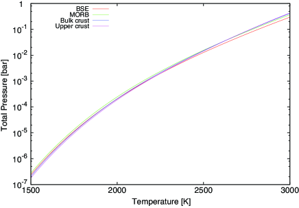
Figure 1.— Total pressures of gas in gas/melt equilibrium with magma of assumed composition are shown as functions of temperature. The assumed bulk compositions are the same as those of the bulk silicate Earth (BSE) (red), the Earth’s mid-ocean ridge basalts (MORB) (green), the Earth’s bulk crust (blue), and the Earth’s upper crust (magenta) (see Table 1 for the details).

(a) BSE

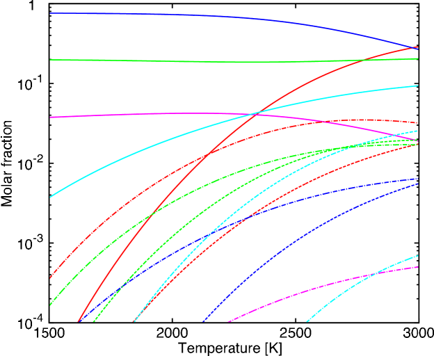
(b) MORB

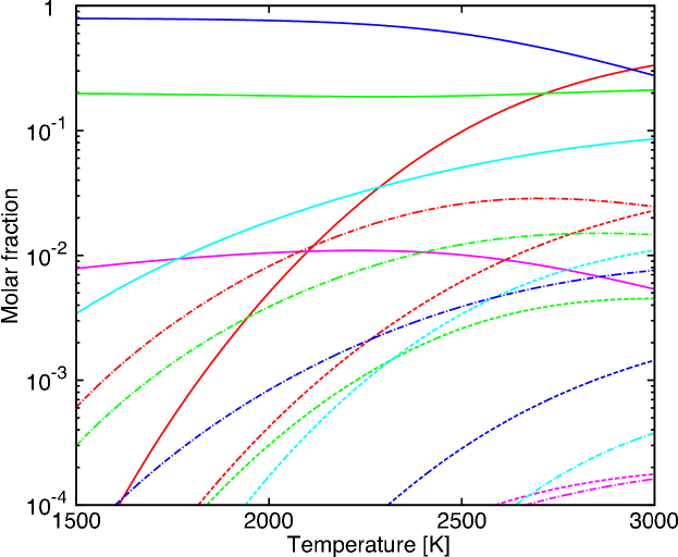
(c) Bulk crust

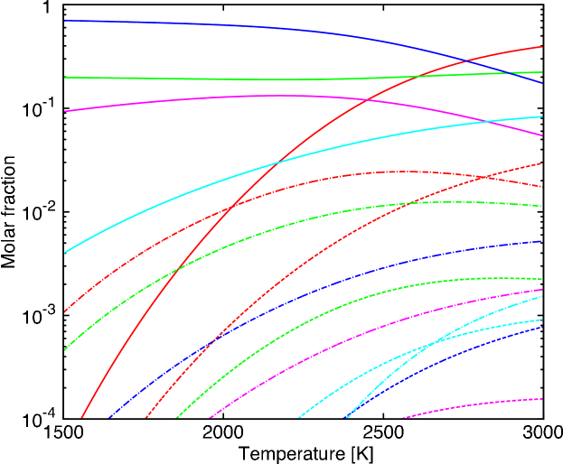
(d) Upper crust

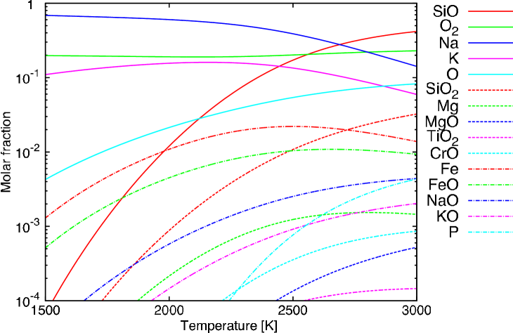
Figure 2.— Composition of gas in chemical equilibrium with molten silicate. Molar fractions of the gas species are shown as functions of temperature. The assumed bulk compositions are the same as those of (a) the bulk silicate Earth (BSE), (b) the Earth’s mid-ocean ridge basalts (MORB), (c) the Earth’s bulk crust, and (d) the Earth’s upper crust (see Table 1 for the details).

2.2. Gas phase equilibrium

To calculate the equilibrium abundances of gas species in the mineral atmosphere, we use the NASA CEA code (Gordon & McBride, 1996), which performs the free-energy minimization calculations. In practice, we calculate the abundances for some selected temperatures from 2000 K to 4500 K and pressures from 10^-8 bar to 10^-1 bar, which are of interest in this study, considering the gas phase equilibrium of a system composed of only the major elements such as O, Na, K, Si and Fe. We assume that the element abundances are vertically constant; their values are calculated in section 2.1.

In our atmosphere model, the molar fractions of Na, K and Fe gas vary little, compared to those of O, O₂, Si and SiO. O₂ and SiO tend to decrease and O and Si increase with altitude in low pressure regions in the atmosphere (see section 4), because of thermal dissociations of O₂ and SiO.

Although we ignore photo-chemical reactions in this study, the photo-dissociation of SiO may be important for the detectability of the atmosphere. We discuss the possibility of the photo-dissociation of SiO and the impact on the atmospheric structure and detectability in section 6.3.

3. ABSORPTION OPACITY

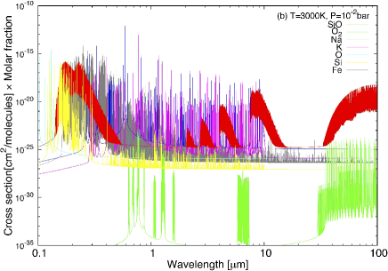
Figure 3.— Absorption cross sections of the seven major gas species, SiO (red), O₂ (green), Na (blue), K (magenta), Fe (grey), O (cyan), and Si(yellow) as functions of wavelength. Each cross section is multiplied by each molar fraction. The magma composition is assumed to be BSE (see Table 1). (a): The temperature is 2000 K and the pressure is $1\times 10^{-5}$ bar. The calculated molar fractions of Na, K, Fe, Si, SiO, O, and O₂ are $0.721$, $0.0407$, $0.001$, $1\times 10^{-6}$, $0.00731$, $0.0233$, and $0.189$, respectively. (b): The temperature is 3000 K and the pressure is $1\times 10^{-2}$ bar. The calculated molar fractions of Na, K, Fe, Si, SiO, O, and O₂ are $0.204$, $0.0142$, $0.01$, $1\times 10^{-3}$, $0.343$, $0.0991$, and $0.211$, respectively.

Among the chemical species shown in Figure 2, we consider line absorption by seven major species that include Na, K, Fe, O, O₂, Si and SiO. We neglect Rayleigh scattering, because the Rayleigh scattering opacities are mostly smaller than the absorption opacity of SiO at wavelengths of interest in this study, as discussed in section 6.1. Note that while TiO is known to be a strong absorber for visible ray (Allard et al., 2000; Plez, 1998), its absorption opacity is always smaller than Na absorption opacity in the visible and IR wavelength regions, because the molar fraction of TiO is negligibly small (e.g., $\sim 10^{-12}$ at $T$ = 1500 K and $\sim 10^{-6}$ at $T$ = 3000 K), compared to that of Na ($\gtrsim$ 0.1) in the atmosphere considered here.

Absorption opacities are calculated in the following way, except for O₂, for which we apply vibrational-rotational transitions in the HITRAN database (Rothman et al., 2013). In local thermodynamic equilibrium, the absorption cross section of species A for an energy transition from the $i$th level to the $j$th level, $\sigma_{\nu}^{\mathrm{A}}(i,j)$, is given as (Piskunov & Kupka, 2001)

$$\sigma^{\mathrm{A}}_{\nu}(i,j)= g_{i}f_{ij}\frac{\pi e^{2}}{m_{e}c}\frac{\exp({-E_{i}/kT})}{Q(T)}$$

$$\times\left\{1-\exp\left(\frac{E_{j}-E_{i}}{kT}\right)\right\}H(\nu,a),$$ (1)

where $\nu$ is the frequency, $g_{i}$ is the statistical weight of the $i$th energy level, $f_{ij}$ is the oscillator strength for a transition from the $i$th (lower) to $j$th (higher) level, $E_{i}$ and $E_{j}$ are excitation energies of the $i$th and $j$th energy levels, respectively, and $Q(T)$ is the partition function of the species at temperature $T$. $e$ is the elementary charge (= $4.803\times 10^{-10}$ esu), $m_{e}$ is the electron mass (= $9.1094\times 10^{-28}$ g), $c$ is the light velocity (= $2.9979246\times 10^{10}$ cm s^-1), and $k$ is the Boltzmann constant (= $1.3806488\times 10^{-16}$ erg K^-1). We take the values of $g_{i},f_{ij}$ and $E_{i}$ from Kurucz (1992) (see also Barton et al. (2013) for SiO). Also we take the values of $Q(T)$ for Na, K, Fe, Si and O from Irwin (1981) and for SiO from Rossi et al. (1985).

The function $H(\nu,a)$ is the line profile function given by (e.g., Rybicki & Lightman, 1986)

$$H(\nu,a)=\frac{V(\nu,a)}{\sqrt{\pi}\Delta\nu_{D}},$$ (2)

where $a$ is the line width parameter, $V(\nu,a)$ is the Voigt function, and $\Delta\nu_{D}$ is the Doppler width given by

$$\Delta\nu_{D}=\frac{\nu_{0}}{c}\sqrt{\frac{2kT}{m_{A}}},$$ (3)

where $m_{A}$ is the mass of the absorber and $\nu_{0}$ is the central frequency of the spectral line. The line width parameter $a$ is calculated with damping constants for natural broadening and van der Waals broadening as (Piskunov & Kupka, 2001)

$$a=\frac{\Gamma_{r}+\Gamma_{W}}{4\pi\Delta\nu_{D}}.$$ (4)

According to Unsold (1955) and Gray (1976), $\Gamma_{r}$ and $\Gamma_{W}$ are given by

$$\Gamma_{r}=0.222\times 10^{14}\lambda^{-2},$$ (5)

$$\Gamma_{W}=17 \times\left(0.3\times 10^{-30}\left[\frac{(l+1)^{2}}{(I-\chi_{j})^{2}}-\frac{(l+1)^{2}}{(I-\chi_{i})^{2}}\right]\right)^{2/5}$$

$$\times v^{3/5}N,$$ (6)

where $\lambda$ is wavelength in nm, $N$ is the total number density of the gas species in cm^-3, $I$ is the ionization potential in eV, $\chi_{i}$ is the excitation potential at the $i$th level in eV, and $l$ is the electric charge. $v$ is the relative thermal velocity defined by

$$v=v^{A}\sqrt{1+\frac{\mu^{A}}{\overline{\mu}}},$$ (7)

where $v^{A}$ is the thermal velocity of the absorber and $\mu^{A}$ and $\overline{\mu}$ are the molecular weight of the absorber and the mean molecular weight, respectively. As for the SiO absorption opacity, we assume $\Gamma_{W}=10^{-7}\times N$, following Kurucz & Avrett (1981). To calculate the line profile $H(\nu,a)$ numerically, we use a polynomial expansion of the Voigt function given by Kuntz (1997). We have confirmed that this approximation yields relative errors of the order of $10^{-4}$, which is small enough for our discussion in this study.

Figure 3 shows the cross section of each species multiplied by each molar fraction as a function of wavelength for $T=$ 2000 K(a) and 3000 K(b), respectively. The assumed pressures are $1.0\times 10^{-5}$ bar for $T$ = 2000 K and 0.01 bar for $T$ = 3000 K. The magma composition is assumed to be BSE. The calculated molar fractions of Na, K, Fe, Si, SiO, O, and O₂ are, respectively, $x_{\mathrm{Na}}=0.721$, $x_{\mathrm{K}}=0.0407$, $x_{\mathrm{Fe}}=0.001$, $x_{\mathrm{Si}}=10^{-6}$, $x_{\mathrm{SiO}}=0.00731$, $x_{\mathrm{O}}=0.0233$, and $x_{\mathrm{O_{2}}}=0.189$ for $T=$ 2000 K(a) and $x_{\mathrm{Na}}=0.204$, $x_{\mathrm{K}}=0.0142$, $x_{\mathrm{Fe}}=0.01$, $x_{\mathrm{Si}}=1\times 10^{-3}$, $x_{\mathrm{SiO}}=0.343$, $x_{\mathrm{O}}=0.0991$, and $x_{\mathrm{O_{2}}}=0.211$ for $T=$ 3000 K(b).

In Fig. 3a, the most abundant species Na (blue) presents a few hundred of strong absorption lines between 0.253 and 10.0 $\mathrm{\mu m}$, including the D line at 0.5893 $\mathrm{\mu m}$. Also, several hundred strong lines of K (magenta) that are distinguishable from the Na lines are also found between 0.286 and 10.0 $\mathrm{\mu m}$, including potassium doublet lines at 0.766 and 0.770 $\mathrm{\mu m}$. While SiO (red) is less abundant by a factor of about 100 than Na, millions of its electron-transition absorption lines dominate in the FUV wavelength region (0.14 - 0.3 $\mathrm{\mu m}$) and its absorption due to rotation-vibration transition dominates in several parts of the IR wavelength region, except narrow line peaks of Na, K and Fe. The O electron-transition absorption (cyan) dominates between 0.10 and 0.13 $\mathrm{\mu m}$. The several thousands lines of Fe (grey) dominates between 0.20 and 0.54 $\mathrm{\mu m}$. Although O₂ (green) is the second most abundant species, its absorption is obscured by the other absorptions except at a narrow range around 30 $\mathrm{\mu m}$. Also, the Si electron-transition absorption (yellow) is obscured by the SiO absorption in both Figs. 3a and 3b and presents many prominent absorption lines between 0.1 and 0.3 $\mathrm{\mu m}$.

In the higher-$T$ case shown in Fig. 3b, the SiO feature is more prominent. The electron-transition absorption in the FUV region is larger by about two orders of magnitude than that in Fig. 3a, because the molar fraction of SiO is larger by two orders of magnitude (see Fig. 2) and comparable with Na at 3000 K. The most remarkable difference in absorption feature between Fig. 3a and Fig. 3b is that the SiO rotation-vibration absorption dominates at all the wavelengths longer than about 3 $\mathrm{\mu m}$, except several hundreds of narrow lines of Na and K. The rises in the peak values of SiO are due to the increase in abundance, while the enhancement of pressure broadening also contributes to the rises in absorption between those peaks.

Other minor species might contribute to the opacity. As for Mg and P present in Fig. 2, we have confirmed that the absorption opacities of these species are negligibly small relative to the SiO absorption opacity in most of the wavelength region of interest, except for narrow ranges between 0.1 and 0.15 $\mu$m. Absorption line data of the diatomic molecules other than SiO in Fig. 2 are unavailable, to our knowledge. Thus, we have ignored their contribution.

Finally, for integrating the thermal structure of the atmosphere in the next section, we use the total absorption opacity, $\kappa_{\nu}$, calculated as

$$\rho\kappa_{\nu}=N\sum_{\mathrm{A}}x_{\mathrm{A}}\sigma^{\mathrm{A}}_{\nu}(i,j),$$ (8)

where $\rho$ is the mass density.

4. TEMPERATURE PROFILE

In this study, we simulate the one-dimensional plane-parallel thermal structure of the atmosphere that is in the radiative, hydrostatic, and chemical equilibrium. To do so, we integrate the so-called two-stream equations with the assumption of quasi-isotropic radiation, adopting the $\delta-$Eddington approximation (Toon et al., 1989):

$$\frac{dF^{+}_{\nu}}{d\tau_{\nu}} = \frac{7}{4}F^{+}_{\nu}+\frac{1}{4}F^{-}_{\nu}-2\pi B_{\nu}(T),$$ (9)

$$\frac{dF^{-}_{\nu}}{d\tau_{\nu}} = -\frac{1}{4}F^{+}_{\nu}-\frac{7}{4}F^{-}_{\nu}+2\pi B_{\nu}(T),$$ (10)

where $F^{+}_{\nu}$ and $F^{-}_{\nu}$ are the upward and downward radiative fluxes, respectively, $B_{\nu}(T)$ is the Planck function, and $\tau_{\nu}$ is the optical depth defined by

$$\frac{d\tau_{\nu}}{dz}=-\kappa_{\nu}\rho,$$ (11)

where $z$ is the altitude. In equations (9) and (10), we have assumed that the single-scattering albedo is 0, because absorption dominates scattering in most of the wavelength region of interest, as described above. The boundary conditions at the top and bottom of the atmosphere are respectively $F^{-}_{\nu}=0$ and $F^{+}_{\nu}=\pi B_{\nu}(T_{\mathrm{g}})$, where $T_{\mathrm{g}}$ is the ground temperature. To solve equations (9) and (10), we have used the widely-used algorithm developed by Toon et al. (1989). According to Toon et al. (1989), the error in the radiative fluxes caused by the two-stream approximation was typically less than 10%, which is small relative to uncertainties in physical properties of exoplanets.

The net radiative flux integrated over all frequencies is constant throughout the atmosphere in radiative equilibrium. For an irradiated atmosphere, the net radiative flux, $F_{\mathrm{net},\nu}$, is written as

$$F_{\mathrm{net},\nu}(\tau_{\nu})=F^{+}_{\nu}(\tau_{\nu})-F^{-}_{\nu}(\tau_{\nu})-\mu_{\ast}F^{\ast}_{\nu}e^{-\tau_{\nu}/\mu_{\ast}},$$ (12)

where $F_{\nu}^{\ast}$ is the incident stellar flux and $\mu_{\ast}$ is the cosine of the zenith angle of the incident stellar radiation. The radiative equilibrium condition is given as

$$\int^{\infty}_{0}F_{\mathrm{net},\nu}\,d\nu=F_{0},$$ (13)

where $F_{0}$ is the constant flux. An HRSE is subject to tidal heating. Its strength depends on orbital and internal properties of the HRSE (Barnes et al., 2010). The detailed consideration of the tidal heating effect is beyond the scope of this study (A brief discussion is made in section 6.4). In this study, we assume $F_{0}$ = 10 W/m² for numerical stability. For $F_{0}<10$ W/m², we have confirmed that choice of $F_{0}$ have little influence on the thermal structure of the atmosphere.

We consider a pressure range from $1\times 10^{-8}$ bar to the pressure at ground level, $P_{\mathrm{g}}$. Note that $P_{\mathrm{g}}$ is determined a posteriori, because $P_{\mathrm{g}}$ is the vapor pressure, which depends on the ground temperature, $T_{\mathrm{g}}$. Numerically, the atmosphere is vertically divided into 50 layers. The layers are prepared so that the size of each layer logarithmically increases with pressure. In addition, to integrate equations (9) and (10), we consider 100 spectral intervals in a frequency range between $1\times$10¹³ and 2$\times$10¹⁵ s^-1 such that the size of each interval logarithmically increases with frequency. We calculate the harmonic mean opacities using cross sections obtained in section 3. The calculation method of the mean opacities is described in Appendix A.

To find the thermal structure of the atmosphere in radiative equilibrium and also in gas-melt chemical equilibrium with the underlying magma ocean, we need three iterative procedures. Firstly, to find the radiative-equilibrium solution for given opacities and molar fractions of atmospheric gases, we integrate the equation of energy conservation,

$$\frac{dT_{n}}{d\widetilde{t}}=\frac{dF_{n}}{dP_{n}},$$ (14)

where $\widetilde{t}$ is a normalized time, $T_{n}$, $P_{n}$ and $F_{n}$ are the temperature, pressure, and net radiative flux in the $n$th layer, respectively. The integration is continued until $\left|F_{n}-F_{0}\right|/F_{0}$ becomes smaller than 1 % in all the layers.

Secondly, once we find the radiative-equilibrium solution, we calculate the opacities that are consistent with temperatures obtained above. In practice, to save memory and cpu time, we have prepared a numerical table in which the harmonic mean opacities (see Appendix A) in 100 spectral intervals are given as functions of $T$, $\log{P}$, and, the mean molecular weight, $\overline{\mu}$: The grids are prepared for $T$ = 2000, 2500, 3000, 3500, 4000, and 4500 K, $\log(P/\mathrm{bar})$ = $-1$, $-2$, $-3$, $-4$, and $-5$, and $\overline{\mu}$ = 25, 30, and 35. In the pressure range from $1\times 10^{-8}$ bar to $1\times 10^{-5}$ bar, we have ignored the pressure dependence of the opacity because $\Gamma_{r}>\Gamma_{W}$ in the range. Note that we have checked that the calculated flux differs by at most 5 %, even if a smaller table with $T$ = 2000, 3000, and 4000 K, $\log(P/\mathrm{bar})$ = $-1$, $-3$, and $-5$, and $\overline{\mu}$ = 25 and 35 is used. The convergence condition is that the temperature in each layer does not vary within less than 1 %.

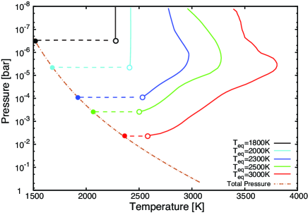
Figure 4.— Temperature-pressure profile in the mineral atmosphere on top of the BSE magma of a super-Earth with gravity of 25 m/s² for five choices of the substellar-point equilibrium temperature, $T_{\mathrm{eq}}$, of 1800 K (black), 2000 K (cyan), 2300 K (blue), 2500 K (green), and 3000 K (red) (see eq. [16]; $A_{p}=0$). The host star is assumed to be a Sun-like star with radius of 1 $R_{\odot}$ and effective temperature of 6000 K and emit the blackbody radiation of 6000 K. The solid lines show the day-side averaged profiles (i.e., the cosine of the stellar-light zenith angle $\mu_{*}=1/2$; see eq. [12]). The open circles show the temperatures at the bottom of the atmosphere, $T_{\mathrm{b}}$, and the filled circles show the temperatures at the ground, $T_{\mathrm{g}}$. The orange dotted line represents the total vapor pressure for the BSE composition, which corresponds to the ground.

(a) $T_{\mathrm{eq}}$ = 1800K

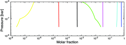
(b) $T_{\mathrm{eq}}$ = 2000K

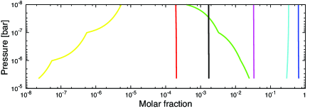
(c) $T_{\mathrm{eq}}$ = 2300K

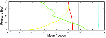
(d) $T_{\mathrm{eq}}$ = 2500K

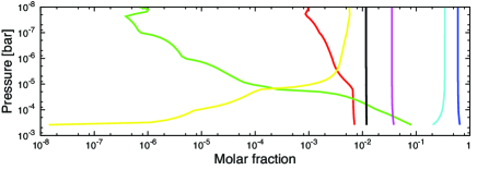
(e) $T_{\mathrm{eq}}$ = 3000K

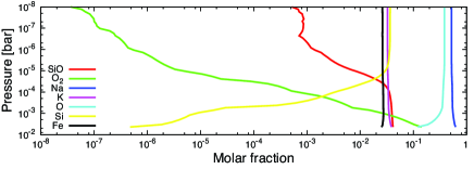
Figure 5.— The distribution of the seven major gas species in chemical equilibrium in the mineral atmosphere. Molar fractions of SiO (red), O₂ (green), Na (blue), K (magenta), Fe (grey), O (cyan) and Si(yellow) are shown as functions of pressure for five choices of the substellar-point equilibrium temperature; (a) $T_{\mathrm{eq}}$ = 1800K, (b) 2000K, (c) 2300K, (d) 2500K, and (e) 3000K. The corresponding temperature-pressure structure of the atmosphere is shown in Figure 4.

Finally, we have to find the solution in which the atmosphere is in equilibrium with the underlying magma ocean at its bottom. The ground pressure $P_{\mathrm{g}}$ and molar fractions $x_{\mathrm{A}}$ are functions of the ground temperature $T_{\mathrm{g}}$ (see section 2). From equations (12) and (13), the magma being assumed to be a blackbody, $T_{\mathrm{g}}$ is given as

$$\sigma T_{\mathrm{g}}^{4}=F_{0}+\int_{0}^{\infty}\left\{F^{-}_{n,\nu}(P_{\mathrm{g}})+\mu_{\ast}F^{\ast}_{\nu}e^{-\tau_{\nu,\mathrm{g}}/\mu_{\ast}}\right\}d\nu,$$ (15)

where $\sigma$ is the Stefan-Boltzmann constant ($=5.67\times 10^{-8}$W/m²K⁴) and $\tau_{\nu,\mathrm{g}}$ is the total optical depth of the atmosphere. We calculate $T_{\mathrm{g}}$ from Eq. (15) and then calculate $P_{\mathrm{g}}$ and $x_{\mathrm{A}}$. The gas chemical equilibrium composition in each layer, $x_{\mathrm{A}}$, is obtained by interpolating linearly the tabulated data made by the NASA CEA code. The grids are prepared for $T$ = 2000, 2500, 3000, 3500, 4000, and 4500 K, $\log(P/\mathrm{bar})$ = $-1$, $-2$, $-3$, $-4$, $-5$, $-6$, $-7$ and $-8$, and $T_{\mathrm{g}}$ being every one kelvin from 1500K to 3000K. The convergence condition is that $T_{\mathrm{g}}$ and the temperature in each layer do not vary within less than 1 %.

Figure 4 shows the calculated temperature profiles for different substellar-point equilibrium temperatures defined by

$$T_{\mathrm{eq}}^{4}=(1-A_{p})\frac{R_{\ast}^{2}}{D^{2}}T_{\ast}^{4},$$ (16)

where $R_{\ast}$ and $T_{\ast}$ are respectively the radius and temperature of the host star, $A_{p}$ is the planetary albedo, and $D$ is the orbital distance of the planet. Five values of $T_{\mathrm{eq}}$ are chosen: $T_{\mathrm{eq}}$ = 1800 K (black), 2000 K (cyan), 2300 K (blue), 2500 K (green), and 3000 K (red). The incident stellar flux is calculated as $F^{\ast}_{\nu}=T_{\mathrm{eq}}^{4}/T_{\ast}^{4}\times\pi B_{\nu}(T_{\ast})$. The solid lines represent the temperature profiles at $\mu_{*}=1/2$ (i.e., day-side average). Also, the open and filled circles show the temperatures at the bottom of the atmosphere, $T_{\mathrm{b}}$, and at the ground, $T_{\mathrm{g}}$, respectively. Figure 5 shows the calculated molar fraction profiles of seven major species for the atmosphere structure shown in Fig. 4. Here we have assumed $g$ = 25 m/s² and $A_{p}$ = 0. The host star is assumed to emit blackbody radiation of 6000 K. The magma composition is assumed to be BSE.

The most remarkable feature of the temperature profiles in Fig. 4 is the thermal inversion structure in the cases of $T_{\mathrm{eq}}\geq 2300$ K. As found in section 3, the absorption is more significant in the UV and visible wavelength regions (0.1 to $\sim$1 $\mathrm{\mu m}$) than in the IR region ($\sim$1 to 4 $\mathrm{\mu m}$), mainly because of the strong UV-ray absorption by SiO and visible-light absorption by the doublet lines of Na and K. (Note that most of the absorption lines of Fe, Na and K are too narrow to contribute to the mean opacity.) This means that the absorption of the incident stellar radiation is stronger compared to the intrinsic planetary radiation, which results in thermal inversion for $P$ $\geq 10^{-5}$bar. For $P$ $\leq 10^{-5}$bar, the temperature decreases with decreasing pressure, because the dissociation of SiO occurs as shown in Figure 5, so that the UV-ray absorption by SiO becomes weak.

Not only the thermal inversion region extends but $T_{\mathrm{g}}$ increases, as $T_{\mathrm{eq}}$ increases. In the case of $T_{\mathrm{eq}}$ = 3000 K, $T_{\mathrm{g}}$, is significantly smaller than $\mu_{*}^{1/4}T_{\mathrm{eq}}$. In contrast, $T_{\mathrm{g}}\simeq\mu_{\ast}^{1/4}T_{\mathrm{eq}}$ for low $T_{\mathrm{eq}}$, because the atmosphere is so optically thin that the ground is directly heated by stellar irradiation. In the cases of $T_{\mathrm{eq}}\leq 2000$ K, the atmosphere is thus isothermal. Note that jumps in temperature between $T_{\mathrm{b}}$ and $T_{\mathrm{g}}$ are found in Figure 4. This is because those atmospheres are optical thin for the incident stellar flux and any heat transfer process except radiative transfer is not taken into account. Thus, in reality, the atmosphere is not exactly isothermal, because there should be a conductive region with steep temperature gradient near the ground. Such structure, however, has little impact on the emission spectra that we use when discussing the detectability of HSREs in secondary eclipse (see section 5).

5. DETECTABILITY VIA SECONDARY ECLIPSE OBSERVATION

5.1. Secondary eclipse depth

Here we assess the detectability of the mineral atmospheres of HRSEs that we have modeled via the secondary eclipse observation. This observation enables us to infer the vertical temperature profile and composition of an exoplanetary atmosphere by obtaining planetary emission spectrum. In particular, the thermal inversion structure found in section 4 is expected to be detected.

The secondary eclipse observation measures the ratio of the planetary luminosity to the sum of the stellar and planetary luminosities. The ratio is often called the secondary eclipse depth, $\epsilon_{\lambda}$, which is given by

$$\epsilon_{\lambda}\simeq\left(\frac{R_{p}}{R_{*}}\right)^{2}\frac{F_{p,\lambda}+A_{p}F_{*,\lambda}}{F_{*,\lambda}},$$ (17)

where $F_{\ast,\lambda}$ is the emergent stellar flux and $F_{p,\lambda}$ is the emergent planetary flux calculated as

$$F_{p,\lambda}=\pi\int^{\infty}_{0}B_{\lambda}(T(\tau_{\lambda}))e^{-\tau_{\lambda}}d\tau_{\lambda}.$$ (18)

Below, as in section 4, we assume $g=25$ m/s², $A_{p}=0$, and blackbody stellar radiation of 6000 K. The magma composition is assumed to be BSE. Also, we suppose an HRSE with radii of 2 $R_{\oplus}$ orbiting a solar analog, namely $R_{p}/R_{\ast}$ = 0.02. To integrate equations (17) and (18), we consider 30000 spectral intervals in the wavelength range between $0.1$ and $100$ $\mathrm{\mu m}$; the size of each interval logarithmically increases with wavelength. Then, as in section 4, we calculate the arithmetic mean opacities, interpolating linearly the tabulated data. We consider only the case of $\mu_{\ast}=1/2$, because we are interested in planetary disk averaged emission (i.e., day-side average).

Figure 6 plots the secondary eclipse depth $\epsilon_{\lambda}$ (and also $F_{p,\lambda}/F_{\ast,\lambda}$) for $T_{\mathrm{eq}}$ = 1800 K (black), 2000 K (cyan), 2300 K (blue), 2500 K (green), and 3000 K (red): Panels (a) and (b) show the spectra in the wavelength region of 0.1–100 $\mathrm{\mu m}$ and 0.3–1 $\mathrm{\mu m}$, respectively. The secondary-eclipse-depth spectra for $T_{\mathrm{eq}}=1800$ K and $2000$ K exhibit only some narrow line features of Na and K. This is mainly because the atmospheres are isothermal (see Fig. 4) except for the temperature jump above the ground. The line features are, thus, due to the emission from parts of the atmosphere with temperatures higher than $T_{\mathrm{g}}$, while the continuous spectra are the black body spectra of $T_{\mathrm{g}}$.

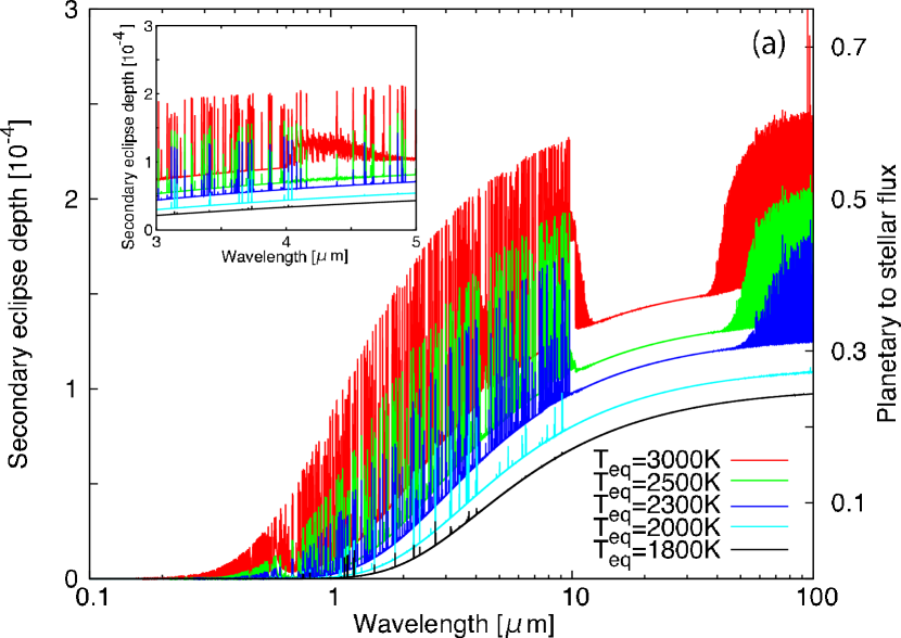
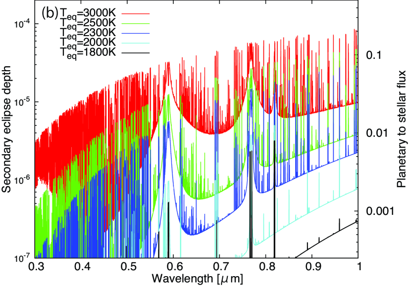
Figure 6.— Predicted dayside-averaged emission spectra of a hot rocky super-Earth of 2 $R_{\oplus}$ in secondary eclipse that has a mineral atmosphere in equilibrium with an underlying BSE magma ocean. The secondary eclipse depth (see eq. [17]) is shown as a function of wavelength in the range of (a) 0.1–100 $\mathrm{\mu m}$ and (b) 0.3–1 $\mathrm{\mu m}$. The inset in the Fig.(a) is an enlarged view of the spectra in 3–5 $\mathrm{\mu m}$. Five equilibrium temperatures are chosen: $T_{\mathrm{eq}}$ = 1800 K (black), 2000 K (cyan), 2300 K (blue), 2500 K (green), and 3000 K (red). The corresponding atmospheric structures are shown by dashed lines in Fig. 4. The host star is assumed to be a Sun-like star with radius of 1 $R_{\odot}$ (i.e., the planetary/stellar radius ratio being 0.02) and emit the blackbody radiation of 6000 K.

By contrast, the spectra for $T_{\mathrm{eq}}=2300$ K and $2500$ K present noticeable features of SiO around 10 and 100 $\mathrm{\mu m}$, in addition to hundreds of narrow features of Na and K. For $T_{\mathrm{eq}}=3000$ K, a spectral feature by SiO around 4 $\mathrm{\mu m}$ appears in addition to those around 10 and 100 $\mathrm{\mu m}$, as shown in the subfigure inside Fig.6a. The features of SiO become stronger as $T_{\mathrm{eq}}$ increases, because the SiO abundance is sensitive to temperature and also the thermal inversion is more significant at higher temperature. Additionally, one can also identify features of the sodium doublet at 0.589 $\mathrm{\mu m}$ and the potassium doublet at 0.77 $\mathrm{\mu m}$ and narrow line features of Fe, Na and K in the visible band, as shown in Panel (b).

5.2. Detectability

We evaluate the detectability of the mineral atmosphere of an HRSE for near-future space-based secondary-eclipse observation. The photometric accuracy of the transit/eclipse observation from space depends on the instrument measurement noise, the intrinsic stellar variability, and the shot noise from photon statistics (e.g. Clanton et al., 2012). In this section, we quantify the photometric accuracy required for the line detection and discuss the feasibility, assuming the ideal case that the total noise is dominated by the shot noise (i.e. the photon-noise limit). To quantify the detectability for the photon-noise limit, we introduce the signal-to-noise ratio of the detection of the secondary eclipse as

$$(S/N)_{\Delta\lambda} = \frac{N_{p}}{\sqrt{N_{*}}},$$ (19)

$$\simeq \epsilon_{\lambda,\Delta\lambda}\sqrt{\frac{At_{\mathrm{obs}}}{\mbox{\char 194}}\frac{R_{*}^{2}}{d^{2}}\frac{\pi B_{\Delta\lambda}(T_{*})}{h}},$$ (20)

where $\Delta\lambda$ is the band width used for the detection of the secondary eclipse, $N_{*}$ is the photon counts of the star, $A$ is the photon collecting area, $t_{\mathrm{obs}}$ is the exposure time, $d$ is the distance of the system, is the resolving power of the spectra, $\epsilon_{\lambda,\Delta\lambda}$ is the depth of the secondary eclipse within $\Delta\lambda$, $N_{p}$ is the photon count of the planet, $B_{\Delta\lambda}(T_{*})$ is the blackbody radiation integrated over a wavelength band (i.e., $\int_{\Delta\lambda}B_{\lambda}(T_{*})d\lambda/\Delta\lambda$), and $h$ is the Planck constant.

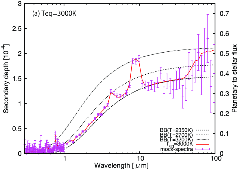
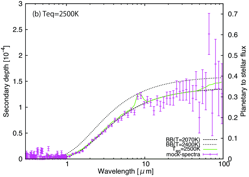
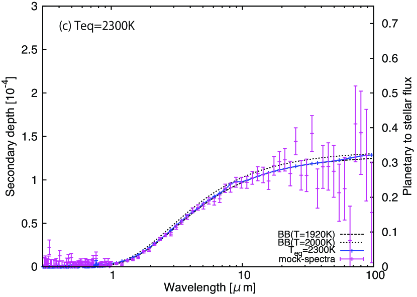
Figure 7.— The secondary eclipse depths theoretically predicted and the mock observational spectrum compared to the blackbody spectra (BB). The secondary eclipse depths are shown as functions of wavelength for $T_{\mathrm{eq}}$ = (a) 3000 K, (b) 2500 K, and (c) 2300 K. The black dotted lines show the secondary eclipse depths of the blackbody, temperatures of which are indicated by ”BB($T$)”. The bars show the mock spectrum calculated based on the photon-noise limit with the assumptions that $R_{*}$ = 1 $R_{\odot}$, $R_{p}$ = $0.02R_{\odot}$, $A=\pi(5\mathrm{m}/2)^{2}$, $t_{\mathrm{obs}}$ = 10 hours, = 100 in 0.3-1 $\mathrm{\mu m}$ and 10 in 1-100 $\mathrm{\mu m}$, and $d$ = 100 pc (see the text for the details). The corresponding atmospheric structures are shown by dashed lines in Fig. 4.

Figure 7 plots the theoretical (solid line), mock (cross), and blackbody (dotted lines) secondary-eclipse-depth spectra for $T_{\mathrm{eq}}$ = 3000 K (a), 2500 K (b), and 2300 K (c). When calculating the mock spectra, we use the false normal random number generation circuit (William et al., 1996), and include the statistical noise, assuming the normal distribution with the standard deviation $\sigma=\sqrt{N_{*}}$. We assume $A=(5/2\,{\rm m})^{2}$ as a fiducial value, roughly corresponding to that of James Webb Space Telescope (JWST; Clampin, 2008), and that = 100 in 0.3-1 $\mathrm{\mu m}$ and 10 in 1-100 $\mathrm{\mu m}$, $t_{\mathrm{obs}}$ = 10 hours, and $d$ = 100 pc. The blackbody spectra are calculated from equation (17) with the assumption $F_{p,\lambda}$ = $B_{\lambda}(T)$.

As demonstrated in Fig. 7, the spectral features of Na, K and SiO are represented by the blackbody spectra with different temperatures (i.e., brightness temperature $T_{\mathrm{br}}$). For example, in the case of $T_{\mathrm{eq}}$ = 3000 K (see Fig. 7a), $T_{\mathrm{br}}$ $\simeq$ 3200 K at 10$\mathrm{\mu m}$, and 2700 K at 4$\mathrm{\mu m}$ due to SiO. Additionally, although not shown, $T_{\mathrm{br}}$ $\simeq$ 3500 K at 0.6 $\mathrm{\mu m}$ and at 0.8$\mathrm{\mu m}$ (which are due to Na and K, respectively), and 3100 K at 100 $\mathrm{\mu m}$ (SiO). At the other wavelengths, $T_{\mathrm{br}}\simeq T_{\mathrm{g}}$ (e.g., $T_{\mathrm{br}}$ = 2350 K for $T_{\mathrm{eq}}$ = 3000 K), because the atmosphere is optically thin at those wavelengths.

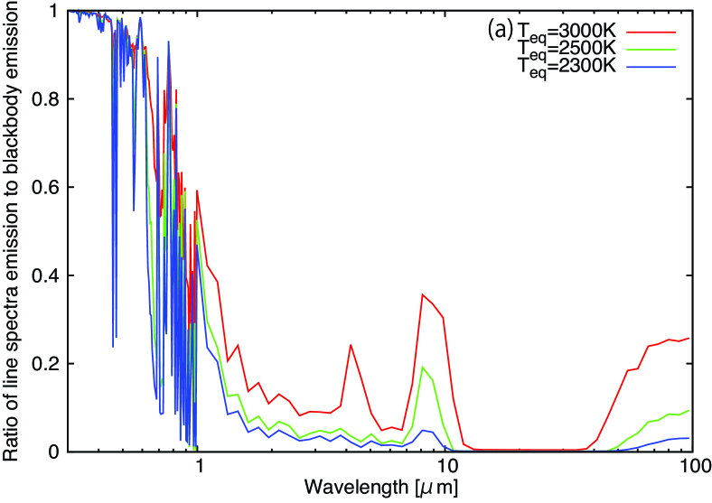
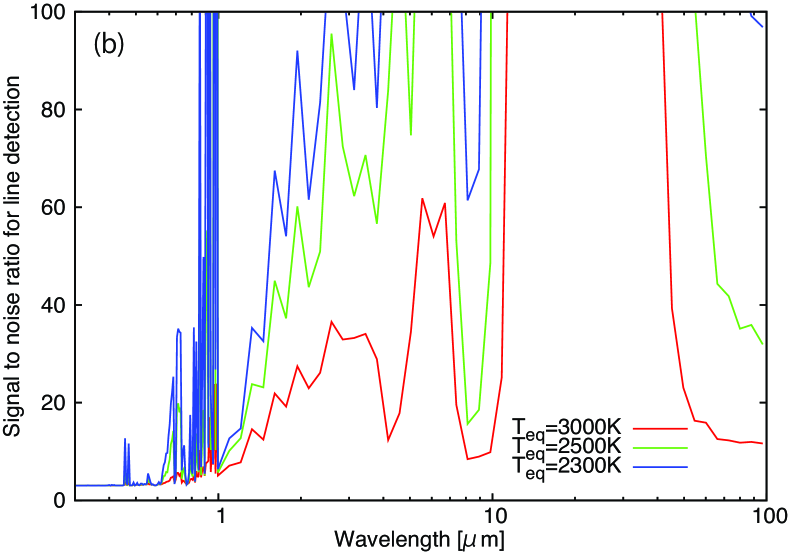
Figure 8.— (a) The secondary eclipse depth relative to that of blackbody with $T_{\mathrm{g}}$ ($\eta_{\lambda,\Delta\lambda}$; see eq. [21]) and (b) the minimum signal-to-noise ratio required to distinguish the emission spectral features from the blackbody emission with $T_{\mathrm{g}}$ ($|(S/N)_{\Delta\lambda}|_{\mathrm{min}}$; see eq. [22]). = 100 in 0.3-1 $\mathrm{\mu m}$ and 10 in 1-100 $\mathrm{\mu m}$. Three equilibrium temperatures are chosen: $T_{\mathrm{eq}}$ = 3000 K (red), 2500 K (green), 2300 K (blue). The corresponding atmospheric structures are shown by dashed lines in Fig. 4. The host star is assumed to be a Sun-like star with radius of 1 $R_{\odot}$ (i.e., the planetary/stellar radius ratio being 0.02) and emit the blackbody radiation of 6000 K.

Comparing the mock spectra with the blackbody spectra, one can quantify the detectability of the spectral features of Na, K and SiO. The error bars become larger in both shorter and longer wavelength regions, because the number of incident photons (i.e., $B_{\Delta\lambda}(T_{*})$) is small in such wavelength regions. Also, the values of , which are assumed to be 100 in 0.1-1 $\mathrm{\mu m}$ and 10 in 1-100 $\mathrm{\mu m}$, affect the value of $(S/N)_{\Delta\lambda}$. As shown in Figure  7a, the spectral features of SiO are sufficiently detectable at 4, 10 and 100 $\mathrm{\mu m}$ for $T_{\mathrm{eq}}$ = 3000 K. The SiO feature is also sufficiently detectable at 10 $\mathrm{\mu m}$ for $T_{\mathrm{eq}}$ = 2500 K (Fig. 7b), while the feature is marginally undetectable for $T_{\mathrm{eq}}$ = 2300 K (Fig. 7c).

The signal-to-noise ratio for detecting the line absorption spectral feature of the secondary eclipse depth is generally smaller than that for the secondary eclipse detection. Thus, we define the secondary eclipse depth relative to that with no atmospheric feature (i.e., blackbody with $T_{\mathrm{g}}$), $\eta_{\lambda,\Delta\lambda}$ as

$$\eta_{\lambda,\Delta\lambda}\equiv\left|\int^{\lambda+\Delta\lambda}_{\lambda}\frac{\epsilon_{\lambda}-\epsilon_{\mathrm{BB},\lambda}(T_{\mathrm{g}})}{\epsilon_{\lambda}}\frac{d\lambda}{\Delta\lambda}\right|,$$ (21)

where $\epsilon_{\mathrm{BB,\lambda}}(T_{\mathrm{g}})$ is the secondary eclipse depth by the blackbody radiation with $T_{\mathrm{g}}$. Using $\eta_{\lambda,\Delta\lambda}$, we estimate the detectability of the line spectral features. From equations (20) and (21), we introduce a new quality, $(S/N)_{L,{\Delta\lambda}}$, that is defined as

$$(S/N)_{L,{\Delta\lambda}} = \eta_{\lambda,\Delta\lambda}(S/N)_{\Delta\lambda}.$$ (22)

When $(S/N)_{L,{\Delta\lambda}}$ is sufficiently large, we can detect the line spectral feature of the secondary eclipse depth. Thus, if the minimum value of $(S/N)_{L,{\Delta\lambda}}$ required to detect a line spectral feature, $|(S/N)_{L,{\Delta\lambda}}|_{\mathrm{min}}$, is 3, $(S/N)_{\Delta\lambda}\geq 3/\eta_{\lambda,\Delta\lambda}$ is required to do so.

Figure 8a shows $\eta_{\lambda,\Delta\lambda}$ for $T_{\mathrm{eq}}$ = 3000 K (red), 2500 K (green), and 2300 K (blue) with = 100 in 0.3-1 $\mathrm{\mu m}$ and 10 in 1-100 $\rm{\mu}$m. As shown in Figure 8a, $\eta_{\lambda,\Delta\lambda}$ takes large values at some wavelengths, because of the strong line features: $\eta_{\lambda,\Delta\lambda}\sim$ 1 at 0.6 $\mathrm{\mu m}$ (Na) and $\sim$ 0.35 at 10 $\mathrm{\mu m}$ (SiO) for $T_{\mathrm{eq}}$ = 3000 K (red). $\eta_{\lambda,\Delta\lambda}$ is large at $\sim$ 4 $\mathrm{\mu m}$ because of the SiO feature peak only for $T_{\mathrm{eq}}$ = 3000 K (red), since the SiO feature is weaker than Na and K features for $T_{\mathrm{eq}}$ = 2300 K and 2500 K. Also, Figure 8b shows $|(S/N)_{L,{\Delta\lambda}}|_{\mathrm{min}}/\eta_{\lambda,\Delta\lambda}(\equiv|(S/N)_{\Delta\lambda}|_{\mathrm{min}}$) for $T_{\mathrm{eq}}$ = 3000 K (red), 2500 K (green), and 2300 K (blue), assuming $|(S/N)_{L,{\Delta\lambda}}|_{\mathrm{min}}$ = 3 as a minimum fiducial value to detect the line spectral feature with = 100 in 0.3-1 $\mathrm{\mu m}$ and 10 in 1-100 $\mathrm{\mu m}$. We obtain that $|(S/N)_{\Delta\lambda}|_{\mathrm{min}}\lesssim$ 100 around 4, 10 and 100 $\mathrm{\mu m}$; for example, $|(S/N)_{\Delta\lambda}|_{\mathrm{min}}$ $\simeq$ 60 at 10 $\mathrm{\mu m}$ for $T_{\mathrm{eq}}$ = 2300 K (blue) and $|(S/N)_{\Delta\lambda}|_{\mathrm{min}}\simeq$ 10 at 4 $\mathrm{\mu m}$ for $T_{\mathrm{eq}}$ = 3000 K (red). Thus, observation of an HRSE in secondary eclipse can detect the components of the mineral atmosphere such as Na, K and SiO, provided its signal to noise ratio is larger than $|(S/N)_{\Delta\lambda}|_{\mathrm{min}}$.

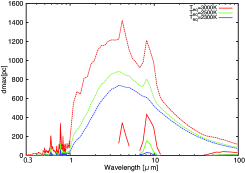
Figure 9.— The limiting distance $d_{\mathrm{max}}$ (see eq. [23] for the definition), interior to which an HRSE with the model atmosphere orbiting a Sun-like star is detectable with $(S/N)_{\Delta\lambda}$ by a given instrument, is shown as a function of wavelength for three equilibrium temperatures $T_{\mathrm{eq}}$ = 3000 K (red), 2500 K (green), and 2300 K (blue) with the assumption that $R_{*}$ = 1 $R_{\odot}$, $R_{p}$ = $0.02R_{\odot}$, $A=\pi(5\mathrm{m}/2)^{2}$, $t_{\mathrm{obs}}$ = 10 hours, and = 10 in 1-100 $\mathrm{\mu m}$ and 100 in 0.3-1 $\mathrm{\mu m}$. The corresponding atmospheric structure is shown in Fig. 4. The solid lines show the limiting distance $d_{\mathrm{max}}$ to detect the line spectral features within secondary eclipse depth around 4, 10, and 100 $\mathrm{\mu m}$, assuming $(S/N)_{\Delta\lambda}=3/\eta$ shown in Figure 8b. The dotted lines show the limiting distance $d_{\mathrm{max}}$ to detect the secondary eclipse depth itself, assuming $(S/N)_{\Delta\lambda}$=3. The host star is assumed to be a Sun-like star with radius of 1 $R_{\odot}$ (i.e., the planetary/stellar radius ratio being 0.02) and emit the blackbody radiation of 6000 K.

Finally, we estimate the limiting distance $d_{\mathrm{max}}$ interior to which an HRSE with the mineral atmosphere is detectable with a given $|(S/N)_{\Delta\lambda}|_{\mathrm{min}}$, for the photon-noise limiting case. From equation (20), $d_{\mathrm{max}}$ is written as

$$d_{\mathrm{max}}\left\{|(S/N)_{\Delta\lambda}|_{\mathrm{min}}\right\} = \frac{\epsilon_{\lambda,\Delta\lambda}}{|(S/N)_{\Delta\lambda}|_{\mathrm{min}}}$$ (23)

$$\times\sqrt{\frac{At_{\mathrm{obs}}}{\mbox{\char 194}}\frac{\pi B_{\Delta\lambda}(T_{*})}{h}}R_{*}.$$

Figure 9 shows $d_{\mathrm{max}}$ as a function of wavelength for $|(S/N)_{\Delta\lambda}|_{\mathrm{min}}$ = $3/\eta_{\lambda,\Delta\lambda}$ (i.e., the minimum signal-to-noise ratio for the detection of line spectral features within secondary eclipse depth; shown by solid lines) or $3$ (i.e., the minimum signal-to-noise ratio for the detection of the secondary eclipse depth itself; shown by dotted lines); $R_{*}$ = 1 $R_{\odot}$, $R_{p}$ = $0.02R_{\odot}$, $A=\pi(5\mathrm{m}/2)^{2}$, $t_{\mathrm{obs}}$ = 10 hours, and = 10 in 1-100 $\mathrm{\mu m}$ and 100 in 0.3-1 $\mathrm{\mu m}$. In particular, the solid lines show the limiting distance $d_{\mathrm{max}}$ to detect the SiO line spectral features around 4, 10, and 100 $\mathrm{\mu m}$. Note that $d_{\mathrm{max}}$ around 4 $\mathrm{\mu m}$ is not shown for $T_{\mathrm{eq}}$ = 2300 K and 2500 K, because the Na, K and SiO features in those cases are indistinguishable from each other when integrating the secondary eclipse depth with respect to wavelength with = 10.

Table 2 summarizes $d_{\mathrm{max}}$ for the SiO detection. The limiting distance $d_{\mathrm{max}}$ increases with increasing $T_{\mathrm{eq}}$, because an HRSE with higher $T_{\mathrm{eq}}$ shows greater planetary emission and more remarkable line absorption spectral feature of the secondary eclipse depths. Thus, the mineral atmospheres of more distant HRSEs would be also detectable if they have higher $T_{\mathrm{eq}}$.

Table 2Limiting distance for detection of the SiO line features

$d_{\mathrm{max}}$	$T_{\mathrm{eq}}$ = 2300 K	$T_{\mathrm{eq}}$ = 2500 K	$T_{\mathrm{eq}}$ = 3000 K
4$\mathrm{\mu m}$	-	-	340pc
10$\mathrm{\mu m}$	30pc	150pc	430pc
100$\mathrm{\mu m}$	3.5pc	8.7pc	40pc

5.3. Application to known HRSEs

We show the simulated secondary-eclipse-depth spectra of four known close-in super-Earths, CoRoT-7b, Kepler-10b, Kepler-78b, and 55 Cnc e in Fig. 10. Within the 1$\sigma$ errors of their observed masses and radii, it is possible that those super-Earths are naked rocky planets. Note that, according to Dragomir et al. (2014), the 1$\sigma$ upper limit on the measured 55 Cnc e’s density just reaches the pure rock regime. If so, they have mineral atmospheres, because of high $T_{\mathrm{eq}}$ (see Table 3). In the simulations, we have assumed = 10 in 1-100 $\mathrm{\mu m}$ and 100 in 0.3-1 $\mathrm{\mu m}$. The values of the planetary and stellar parameters that we have used are listed in Table 3.

The secondary eclipse depth becomes large, as $R_{p}$/$R_{\ast}$ increases and $T_{\mathrm{eq}}$ increases. Thus, the secondary eclipse depth of 55 Cnc e ($R_{p}/R_{\ast}$ = 2.12 $R_{\oplus}$/$R_{\odot}$) is largest, while that of Kepler-10b ($R_{p}/R_{\ast}$ = 1.39 $R_{\oplus}$/$R_{\odot}$) is smallest. Despite of its larger $R_{p}/R_{\ast}$, the secondary eclipse depth of CoRoT-7b is smaller than that of Kepler-78b, because $T_{\mathrm{eq}}$ of CoRoT-7b is smaller than that of Kepler-78b.

Prominent absorption features are found around $\lambda=$ 0.6 $\mathrm{\mu m}$ (Na), 0.77 $\mathrm{\mu m}$ (K), 4 $\mathrm{\mu m}$, 10 $\mathrm{\mu m}$ and 100 $\mathrm{\mu m}$ (SiO). In particular, in the cases of Kepler-10b and 55 Cnc e, those features would be detectable by the near-future space-based observation that we have assumed in subsection 5.2, because the distances of these systems are shorter than ($R_{*}$/$R_{\odot}$)^-1 ($R_{p}$/$2R_{\oplus}$)² $d_{\mathrm{max}}$ from equations (17) and (23).

Table 3Assumed planetary and stellar parameters

	Corot-7ba	Kepler-10bb	Kepler-78bc	55 Cnc ed
$M_{p}$	7.42 $M_{\oplus}$	3.33 $M_{\oplus}$	1.69 $M_{\oplus}$	8.09 $M_{\oplus}$
$R_{p}$	1.58 $R_{\oplus}$	1.47 $R_{\oplus}$	1.20 $R_{\oplus}$	1.99 $R_{\oplus}$
$D$	$0.0172$AU	0.0168 AU	0.0092 AU	0.0155 AU
$T_{\mathrm{eq}}$	2550 K	3090 K	3000 K	2700 K
$R_{*}$	0.82 $R_{\odot}$	1.06 $R_{\odot}$	0.74 $R_{\odot}$	0.94 $R_{\odot}$
$T_{*}$	5250 K	5700 K	5200 K	5200 K
distance	150pc	173pc	-	12.3pc

Notes. Hatzes et al. (2011); Bruntt et al. (2010); Léger et al. (2009), Dumusque et al. (2014); Fressin et al. (2011), Howard et al. (2013), Dragomir et al. (2014); Nelson et al. (2014); Ehrenreich et al. (2012)

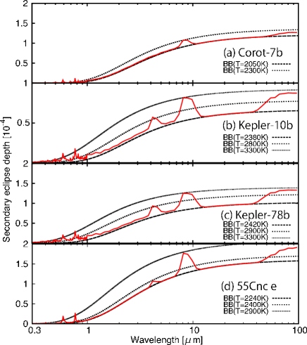
Figure 10.— The secondary eclipse depths theoretically predicted for (a) Corot-7 b, (b) Kepler-10 b, (c) Kepler-78 b and (d) 55 Cnc e, shown as a function of wavelength, assuming that they have the mineral atmosphere. The solid lines show the predicted secondary eclipse depth. The black dotted lines show the secondary eclipse depths of the blackbody, temperatures of which are indicated by ”BB($T$)”. We have assumed = 100 in 0.3-1 $\mathrm{\mu m}$ and 10 in 1-100 $\mathrm{\mu m}$ and the planets’ parameters shown in Table 3.

Demory et al. (2012) have already reported the detection of the secondary eclipse depth of 55 Cnc e with Spitzer Space Telescope at 4.5 $\mu$m. The measured brightness temperature of 2360 $\pm$ 300 K is consistent with our result shown in Fig. 10(d), although the error is large. Also, the SiO IR-absorption features of an HRSE that is brighter and closer than 55 Cnc e would be detectable with Spitzer in the IRAC 4.5 and 8 $\mu$m channel.

Table 4Values of the line contrast

the line contrast $C_{L,(\lambda,\Delta\lambda)}$	$T_{\mathrm{eq}}$ = 2300 K	$T_{\mathrm{eq}}$ = 2500 K	$T_{\mathrm{eq}}$ = 3000 K	55 Cnc e	Accuracy of EChO
Na at 0.59 $\mathrm{\mu m}$	4.4ppm	9.3ppm	26ppm	19ppm ( = 100)	-
K at 0.77 $\mathrm{\mu m}$	6.4ppm	14ppm	36ppm	26ppm ( = 100)	-
SiO at 4 $\mathrm{\mu m}$	-	-	30ppm	16ppm ( = 50)	12ppm ( = 50)
SiO at 10 $\mathrm{\mu m}$	4.6ppm	24ppm	67ppm	54ppm ( = 30)	24ppm ( = 30)
SiO at 100 $\mathrm{\mu m}$	4.0ppm	13ppm	50ppm	36ppm ( = 30)	-

Using equations (20) and (21), we define the line contrast to the total flux, $C_{L,(\lambda,\Delta\lambda)}$ as

$$C_{L,(\lambda,\Delta\lambda)}\equiv\eta_{\lambda,\Delta\lambda}\,\epsilon_{\lambda,\Delta\lambda}.$$ (24)

The photometric accuracy should be smaller than $C_{L,(\lambda,\Delta\lambda)}$ in order to detect the line spectra feature of the secondary eclipse depth. There are several proposed missions that aim to characterize transiting exoplanets, such as Fast Infrared Exoplanet Spectroscopy Survey Explorer (FINESSE; e.g. Deroo et al., 2012) and the Exoplanet Characterization Observatory (EChO; e.g. Tinetti et al., 2012). Here we compare our results with the accuracy of EChO. Figure 11 shows the theoretical (solid line) and mock-EChO (bars) secondary-eclipse-depth spectra for a super-Earth with a mineral atmosphere, using 55 Cnc e’s parameters. Then, we create the mock-EChO spectra with of 50 in 1–5 $\mathrm{\mu m}$ and 30 in 5–16 $\mathrm{\mu m}$, and the photometric accuracy of EChO in Chemical census mode (Waldmann & Pascale, 2014) . Our result demonstrates that EChO has enough accuracy to detect the SiO feature of the mineral atmosphere of 55 Cnc e around 4 $\mathrm{\mu m}$ and 10 $\mathrm{\mu m}$.

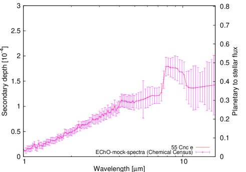
Figure 11.— The secondary eclipse depths theoretically predicted and the mock-EChO observational spectrum for 55 Cnc e with the mineral atmosphere. The secondary eclipse depth is shown as a function of wavelength. The solid line shows the predicted secondary eclipse depth. The magenta bars show the mock-EChO observational spectrum (Waldmann & Pascale, 2014). We have assumed = 50 in 1-5 $\mathrm{\mu m}$ and 30 in 5-16 $\mathrm{\mu m}$ and 55 Cnc e’s parameters: $M_{p}$ = 8.09 $M_{\oplus}$, $R_{p}$ = 1.99 $R_{\oplus}$, $a$ = $0.0155$AU, $T_{\mathrm{eq}}$ = 2700 K $R_{*}$=0.94 $R_{\odot}$ and $T_{*}$=5200K.

Table 4 shows the line contrasts $C_{L}$ of Na (0.59 $\mathrm{\mu m}$), K (0.77 $\mathrm{\mu m}$) and SiO (4 $\mathrm{\mu m}$, 10 $\mathrm{\mu m}$ and 100 $\mathrm{\mu m}$) for $T_{\mathrm{eq}}$ = 2300 K, 2500 K, and 3000 K ( = 100 for $\lambda\leq$ 1 $\mathrm{\mu m}$ and = 10 for $\lambda\geq$ 1 $\mathrm{\mu m}$), and 55 Cnc e’s parameters ( = 100 for $\lambda\leq$ 1 $\mathrm{\mu m}$, = 50 for 1 $\mathrm{\mu m}$ $\leq$ $\lambda\leq$ 5 $\mathrm{\mu m}$ and = 30 for $\lambda\geq$ 5 $\mathrm{\mu m}$). The photometric accuracy of EChO in Chemical Census mode of 55 Cnc e (Waldmann & Pascale, 2014) is also shown in Table 4. Note that the values of $C_{L}$ at 4 $\mathrm{\mu m}$ are not shown for $T_{\mathrm{eq}}$ = 2300 K and 2500 K, because the Na, K and SiO features in those cases are indistinguishable with = 10. We obtain that $C_{L,(\lambda,\Delta\lambda)}$ $\gtrsim$ 10 ppm for Na (0.59 $\mathrm{\mu m}$), K (0.77 $\mathrm{\mu m}$) and SiO (4 $\mathrm{\mu m}$, 10 $\mathrm{\mu m}$ and 100 $\mathrm{\mu m}$); for example, $C_{L,(\lambda,\Delta\lambda)}$ $\sim$ 14 ppm at 0.77 $\mathrm{\mu m}$ and 24 ppm at 10 $\mathrm{\mu m}$ for $T_{\mathrm{eq}}$ = 2500 K and $C_{L,(\lambda,\Delta\lambda)}$ $\sim$ 26 ppm at 0.59 $\mathrm{\mu m}$, 34 ppm at 0.77 $\mathrm{\mu m}$, and 67 ppm at 10 $\mathrm{\mu m}$ for $T_{\mathrm{eq}}$ = 3000 K. The required photometric accuracy to detect the SiO features at 4 and 10 $\mathrm{\mu m}$ is achievable with the Chemical Census mode of EChO for 55 Cnc e.

5.4. How many HRSEs are detectable via near-future observation?

The Kepler space telescope discovered 4250 planet candidates (http://exoplanets.org, as of 30 Nov. 2014). The Kepler Objects of Interest (KOIs) include super-Earth-size objects with short periods (i.e., HRSEs), in particular, 751 objects with $R_{p}\leq 2R_{\oplus}$ orbiting stars with $T_{\mathrm{eff}}$ = 5300-6000 K. Among them, there are 60 KOIs with $T_{\mathrm{eq}}>$ 2300 K. If they are naked rocky planets, their mineral atmospheres can be identified by secondary-eclipse observations with sufficient signal-to-noise ratios. We estimate the expected number of such HRSEs detectable by near future observations.

Assuming a uniform distribution of G-type stars, the number of the detectable HRSEs, $\overline{N_{\mathrm{HRSE}}}$, is given by

$$\overline{N_{\mathrm{HRSE}}}\approx rN_{\mathrm{G}}\frac{4\pi}{3}\left[d_{\mathrm{max}}\left\{(S/N)_{\Delta\lambda}\right\}\right]^{3},$$ (25)

where $r$ is the occurrence rate of HRSEs with $T_{\mathrm{eq}}\geq 2300$ K hosted by G-type stars and $N_{\mathrm{G}}$ is the number density of G-type stars. The HRSEs with $T_{\mathrm{eq}}\geq 2300$ K, which should exhibit the prominent emission features (Fig. 7), correspond to planets with period $P\lesssim 2$ days around G-type stars. Fressin et al. (2013) estimated, using KOI host stars, the occurrence rate of planets with $1.25R_{\oplus}<R_{p}<2R_{\oplus}$ hosted by G-type stars to be close to $0.35$. They also estimated the occurrence rate of planets with $1.25R_{\oplus}<R_{p}<2R_{\oplus}$ and $0.8<P<2$ days to be $1.7(\pm 0.3)\times 10^{-3}$. Using their results, the occurrence rate of the planets with $1.25R_{\oplus}<R_{p}<2R_{\oplus}$ and $0.8<P<2$ days hosted by G-type stars is estimated to be $r\sim 6\times 10^{-4}$. Here we use $r$ = $6\times 10^{-4}$ as a fiducial value of the occurrence rate.

In section 5.2, we estimated ${d_{\mathrm{max}}}\left\{(S/N)_{\Delta\lambda}=3/\eta_{\lambda,\Delta\lambda}\right\}$ to be 430 pc ($T_{\mathrm{eq}}$ = 3000 K), 150 pc ($T_{\mathrm{eq}}$ = 2500 K) and 30 pc ($T_{\mathrm{eq}}$ = 2300 K) for 10 $\mathrm{\mu m}$ observation (see Fig. 9 and Table 2). These HRSEs with $T_{\mathrm{eq}}=2300$ K, $2500$ K and $3000$ K have the orbital period $P\sim 0.93$, 1.6 and 2.0 days, respectively. Hence we take the simple mean $\left[(430^{3}+150^{3}+30^{3})/3\right]^{1/3}\rm{pc}\sim 300\,{\rm pc}$ as a fiducial value of the limiting distance for HRSEs with $0.8<P<2$ days. Inputting $r=6\times 10^{-4}$ % and $N_{\mathrm{G}}$ $\sim$ $6$$\times 10^{-3}\mathrm{pc}^{-3}$ (see a recent review by Traub & Oppenheimer, 2011) in equation (25), we find that within 300 pc there are approximately 400 HRSEs whose 10 $\mathrm{\mu m}$ SiO features are detectable . Taking the transiting probability of $\sim$ 0.2 ($\sim R_{\odot}/D$ for $P=$ 1.3 days) into account, one will be able to detect the 10 $\mathrm{\mu m}$ SiO features from $\sim$ 80 transiting HRSEs by a 5 m space telescope equipped with a photon-noise limited instrument.

6. MODEL VALIDATION AND FUTURE STUDY

6.1. Scattering

In this study, we have ignored the effect of scattering on the thermal structure of the mineral atmosphere. There are two possible sources for scattering. One is Rayleigh scattering by the major gases. The cross section for Rayleigh-scattering by gas species A, $\sigma_{s,\nu}^{A}$, ignoring the polarizability anisotropy, are approximately given as (e.g., CRC Handbook, 2011)

$$\sigma_{s,\nu}^{A}=\frac{8\pi}{3c^{4}}(2\pi\nu)^{4}\alpha_{A}^{2},$$ (26)

where $\alpha_{A}$ is the static average electric dipole polarizability of gas species A. According to CRC Handbook (2011), $\alpha_{\mathrm{A}}$ for ground-state atoms and diatomic molecules in the unit of $10^{-24}$ cm³ are 24.11 for Na, 43.4 for K, 0.802 for O, and 1.5689 for O₂. While $\alpha_{\mathrm{A}}$ for SiO is unavailable in the literature, to our knowledge, it should not differ by several orders of magnitude from those of the other gases. Comparing the cross sections for Rayleigh scattering by those gases with the total absorption cross section calculated in section 3, we have confirmed that the formers are smaller by several orders of magnitude than the latter in most of the wavelength region of interest, except for the narrow ranges between 0.1 and 0.15 $\mathrm{\mu m}$ and between 0.3 and 0.45 $\mathrm{\mu m}$. We have integrated the thermal structure incorporating the effect of the Rayleigh scattering by Na, which results in only a few percent difference in temperature. Also, the Rayleigh and Mie scattering by cloud particles can affect the thermal structure of the mineral atmosphere, if present. However, since the atmospheric temperature is always higher than the vapor pressure of rock, as shown in Fig. 4, no condensation cloud is formed in the atmosphere.

6.2. Non-LTE effect

The approximation of local thermal equilibrium (LTE) is invalid at low pressures. In this study, we have considered a pressure range of $>1\times 10^{-8}$ bar. For LTE to be attained, thermalization due to atomic/molecular collisions must occur faster than radiative cooling. The collisional timescale, $\tau_{\mathrm{coll}}$, is $\sim$ $kT/(Pv\sigma_{\mathrm{coll}})$, where $\sigma_{coll}$ and $v$ are the collisional cross section and thermal velocity of molecules. For SiO, since $\sigma_{\mathrm{coll}}$ $\approx$ $3\times 10^{-15}$ cm², $T$ $\approx$ 3000 K, $v$ $\approx$ $8\times 10^{4}$ cm/s and the typical radiative-cooling timescale (i.e., the typical lifetime of excited states) $\tau_{\mathrm{cool}}$ $\approx$ $1\times 10^{-2}$ s (Barton et al., 2013), LTE is valid for $P\gtrsim 2\times 10^{-7}$ bar. Since the emission from the low pressure region of $P\lesssim 2\times 10^{-7}$ bar makes little contribution to the secondary eclipse depth, the LTE approximation is valid for the SiO-dominated atmosphere of special interest in this study.

6.3. Photodissociation of SiO

Our equilibrium calculations show that the major gas species in the mineral atmosphere are Na, K, Fe, O, O₂, Si and SiO (section 4). Although having been ignored in this study, photodissociation of SiO would occur in such an atmosphere by irradiation of stellar UV (e.g., Vorypaev, 1981).

Jolicard et al. (1997) provided the photodissociation cross section of SiO, $\sigma_{\mathrm{dis}}$, in the wavelength range between 0.153 $\mathrm{\mu m}$ and 0.157 $\mathrm{\mu m}$, where the cross section decreases monotonically with increasing wavelength from $\sim$10^-17 cm² to 10^-19 cm². The energy of UV rays of $\lambda>$ 0.157 $\mathrm{\mu m}$ is not high enough to dissociate SiO significantly; instead, the electron-transition of SiO is dominant, as discussed in section 3. Also, for $\lambda=$ 0.152-0.163 $\mathrm{\mu m}$, the electron-transition cross section of Si is larger than 10^-17 cm² and thus larger than $\sigma_{\mathrm{dis}}$. Therefore, it is the UV ray of $\lambda\leq$ 0.152 $\mathrm{\mu m}$ that dissociates SiO efficiently in the mineral atmosphere. Although no other published data for $\sigma_{\mathrm{dis}}$ is available, $\sigma_{\mathrm{dis}}$ is unlikely to decrease with decreasing wavelength. Below, we make a rough estimate on the impact of SiO photodissociation on the atmospheric structure and the emission features.

Using $\sigma_{\mathrm{dis}}$ $>$ 1 $\times$ 10^-17 cm² with $x_{\mathrm{SiO}}$ = $1\times 10^{-3}$, $\overline{\mu}$ = $20$ and $g$ = 2500 cm/s^-2, we calculate the SiO-photodissociation optical depth, which is defined by

$$\tau_{\mathrm{dis}}=\frac{x_{\mathrm{SiO}}\sigma_{\mathrm{dis}}}{\overline{\mu}m_{\mathrm{H}}g}P,$$ (27)

where $m_{\mathrm{H}}$ is the proton mass. Then, we find that $\tau_{\mathrm{dis}}=1$ at $P$ $<8\times 10^{-6}$ bar. This means that the atmospheric structure for $P\lesssim 8\times 10^{-6}$ bar is affected significantly by photodissociation of SiO. Since the emission features shown in Fig. 4 arise from the region of $P\gtrsim 3\times 10^{-5}$ bar (see Fig. 6), the emission spectra are unlikely to be affected by the photodissociation. More detailed examination requires photo-chemical calculations done consistently with radiative transfer calculations, which must be a future study.

6.4. Tidal heating

Our atmospheric models do not include the effect of tidal heating, discribed in section 4 ($F_{0}$ = 10 W/m² being assumed). According to Henning et al. (2009), tidal heating dominates stellar irradiation under somewhat extreme circumstances such that the planetary eccentricity, $e$, is larger than 0.1 and the orbital period is less than 2 days. Also, Miguel et al. (2011) showed that addition of tidal heating hardly changes the surface temperature of HRSEs for $e$ = 0.01 and 0.001 and the quality factor of the planet, $Q$, of 200 and 20000. Indeed, although not shown, we have confirmed that there is no significant change in the atmospheric structure for $T_{\mathrm{eq}}$ = 3000 K, by calculating the temperature profiles with $F_{0}=10^{3}$ - $10^{7}$ W/m², being equivalent to tidal heat flux for $e$ = 0.01 and 0.001 and $Q$ = 200 and 20000.

6.5. Temperature jump at the bottom

Allowing the temperature jump would affect the composition of the atmosphere. If we included the thermal conduction, we would have no temperature jump at the bottom in the atmosphere, and would have higher $T_{\mathrm{g}}$ and a thicker atmosphere than our model in this study, which is more detectable. The HRSE atmosphere is thin enough for radiation to heat the atmosphere more effectively than thermal conduction. Thus, although the thermal conduction would change $T_{\mathrm{g}}$ and thus the composition of the atmosphere, it would be ineffective in changing the emission spectra of HRSEs.

6.6. Impact of potassium on thermal structure and detectability

As shown in section 2, our chemical-equilibrium calculations yield much more abundant potassium than Schaefer & Fegley (2009) did. Although not shown, we have confirmed that such difference in K abundance has only a small impact on the thermal structure of the atmosphere: Our calculations have demonstrated that the maximum differences in temperature are $\sim$2.86%, $\sim$2.27% and $\sim$1.89% for $T_{\mathrm{eq}}$ = 3000 K, 2500 K and 2300 K, respectively. Thus, the secondary eclipse depths in the IR region are hardly affected.

A direct impact on the secondary eclipse depth is found at $\lambda$ = 0.77 $\mathrm{\mu m}$. Detecting potassium may be useful for constraining the magma composition, because the potassium abundance is different by one order of magnitude from MORB to the upper crust, as shown in Figure 2.

6.7. Other observation methods to detect mineral atmospheres

Other observation methods for atmospheres of close-in exoplanets include transmission spectroscopy and planetary radial velocity (PRV) measurement, in addition to secondary eclipse observation. It would be, however, difficult to detect the HRSEs’ atmospheres via transmission spectroscopy of the planetary disk because of their small scale height. The part of the HRSE’s atmosphere observed by transmission spectroscopy is the rim where horizontal heat and composition transport between the day side and night side would be important. The examination requires 3-D calculations of atmospheric circulation done consistently with radiative transfer calculations, which must be a future study.

Recently, several molecules in the dayside spectra of hot Jupiters have been successfully detected using the high dispersion spectrograph (Brogi et al., 2012; Rodler et al., 2012; de Kok et al., 2013; Rodler et al., 2013; Birkby et al., 2013; Lockwood et al., 2014). This method utilizes the cross-correlation analysis of the spectra and the model template and directly detects PRV. Here, we estimate the feasibility of the PRV detection of the mineral atmosphere of HRSEs. For the most optimistic case, the signal-to-noise ratio of the PRV is determined by the photon noise,

$$(S/N)_{\mathrm{PRV}}=\sqrt{N_{\mathrm{line}}\zeta}(S/N)_{\Delta\lambda}C_{L,(\lambda,\Delta\lambda)},$$ (28)

where $N_{\mathrm{line}}$ is the effective number of molecular lines available for the detection and $\zeta$ is the total efficiency of the high-dispersion instrument (see Kawahara et al., 2014). Although the determination of the precise value of $N_{\mathrm{line}}$ requires full simulations of the spectra including the terrestrial transmission and the night airglow, we here perform 1st order-of-magnitude estimate of the detectability of the Na and K lines here, assuming a future 30 m-class ground-based telescope.

The number of Na and K lines within the secondary eclipse depth spectrum of an HRSE for $T_{\mathrm{eq}}$ $\geq$ 2300K, $N_{\mathrm{line}}$, is $\sim 100$, the line contrast, $C_{L,(\lambda,\Delta\lambda)}$, is $\sim 0.5$ and the mean value of those depths, $\epsilon_{\lambda}$ is $\sim 10^{-4}$, in the IR wavelength region (1-10$\mu$m), as shown in Fig. 6. The resolving power of the instrument, , is required to be large enough to resolve those Na and K lines. To know this value of , we have reintegrated the secondary eclipse depth for $T_{\mathrm{eq}}$ $=$ 2500K around only several Na and K line peaks in the IR wavelength region (3.70-3.75$\mu$m) by line-by-line calculation. We have confirmed that $\mbox{\char 194}=10^{5}$ is enough to resolve the Na and K lines. Thus, we use $\mbox{\char 194}=10^{5}$ below as a fiducial value of . From equation (25), the distance of the system within which at least one transiting HRSE exists is $\sim 70$pc. Assuming a 30 m telescope with $\zeta=0.1$, we obtain the expected S/N for detecting the Na and K lines,

$$(S/N)_{\mathrm{PRV}}\sim 8\left(\frac{\epsilon_{\lambda}}{10^{-4}}\frac{70\mathrm{pc}}{d}\frac{R_{*}}{1R_{\odot}}\frac{C_{L,(\lambda,\Delta\lambda)}}{0.5}\right)$$

$$\times\left(\frac{N_{\mathrm{line}}}{100}\frac{\zeta}{0.1}\frac{A}{\pi 15^{2}\mathrm{m}^{2}}\frac{t_{\mathrm{obs}}}{10\mathrm{hr}}\frac{10^{5}}{\mbox{\char 194}}\frac{\pi B(T_{\ast})/h}{10^{26}\mathrm{m^{-2}s^{-1}}}\right)^{\frac{1}{2}},$$ (29)

where $10^{26}\mathrm{m^{-2}s^{-1}}$ corresponds to the mean value of $\pi B(T_{\ast})/h$ in the wavelength region between 1 and 10$\mu$m, assuming $T_{\ast}=6000$ K. This order-of-magnitude estimate suggests that it would be possible to detect Na and K in the HRSEs’ atmospheres via PRV measurement in the very large telescope era.

7. SUMMARY AND CONCLUSIONS

In this study, we have examined the detectability of hot rocky super-Earths that have atmospheres in the gas/melt equilibrium with the underlying magma oceans via secondary-eclipse observations. First, we have done gas-melt equilibrium calculations and showed that the major atmospheric species are Na, K, Fe, SiO, O, and O₂ (§ 2). We have called this atmosphere the mineral atmosphere in this study.

Next, for those species, we have compiled the absorption line data available in literature, and calculated their absorption opacities in the wavelength region of 0.1–100 $\mathrm{\mu m}$ (§ 3). We have found that the SiO absorption dominates in the UV and IR wavelength regions, while strong absorption by Na and K is found in the visible region. In this atmospheric gas, the opacity is larger in the UV and visible regions than in the IR region.

Third, using those opacities, we have integrated the thermal structure of the atmosphere (§ 4). The most important finding is that thermal inversion occurs in the atmosphere with relatively high equilibrium temperature (i.e., $\mu_{\ast}^{1/4}T_{\mathrm{eq}}\geq 1900$ K), because the UV and visible absorption by SiO dominates the IR absorption by SiO and others. The presence of thermal inversion has a crucial impact on the detectability via secondary eclipse observation.

Finally, by calculating the ratio of the planetary and stellar emission during secondary eclipse, we have quantified the detectability (§ 5). We have found prominent emission features due to SiO at 4, 10, and 100 $\mathrm{\mu m}$. Comparing our predicted spectrum with a mock spectrum we made, we have demonstrated that the mineral atmosphere of a hot rocky super-Earth of radius 2 $R_{\oplus}$ with $T_{\mathrm{eq}}\gtrsim 2300$ K orbiting a solar analog would be detectable by a 5-m space telescope.

The Transiting Exoplanet Survey Satellite (TESS) is a planned space telescope for NASA’s Explorer program and is dedicated to an all-sky transit survey of exoplanets (Ricker et al., 2010). It is predicted that TESS will discover more than 100 transiting Earth-sized exoplanets with short orbital periods. After discovery of nearby HRSEs, follow-up observations by satellites with large telescopes such as JWST, Spitzer, FINESSE and EChO will open new exotic worlds of the mineral atmospheres.

Appendix A Appendix A: Calculation method of the mean opacities

In this study, we use mean opacities for simulating the atmospheric structure and emission spectra, instead of line-by-line calculations. While we integrate the line opacities of O, O₂, Na, K and Si with wavelength resolution high enough to reproduce line profiles, we use low resolution grids to calculate the mean opacity of SiO, because there are too many absorption lines to reproduce the line profile of SiO in a practical CPU time.

Figure 12 presents how to calculate the mean opacity of SiO when an interval between adjacent lines is less than 1 $\mu$m. When an interval between adjacent lines is smaller than $2\Delta\nu_{D}$ and $2(\Gamma_{r}+\Gamma_{W})$ (see the yellow-colored region in Figure 12), we divide the interval equally into quarters. On the other hand, when an interval is larger than $2\Delta\nu_{D}$ or $2(\Gamma_{r}+\Gamma_{W})$ (see the blue-colored region in Figure 12), we select a total of five grids: $\nu_{0,i}$, $\nu_{0,i+1}$, the larger of $\nu_{0,i}+2\Delta\nu_{D}$ and $\nu_{0,i}+2(\Gamma_{r}+\Gamma_{W})$ ($\equiv\nu_{\ell}$), the smaller of $\nu_{0,i+1}-2\Delta\nu_{D}$ and $\nu_{0,i+1}-2(\Gamma_{r}+\Gamma_{W})$ ($\equiv\nu_{r}$), and a midpoint between $\nu_{0,i}$ and $\nu_{0,i+1}$ ($\equiv\nu_{m}$), where $\nu_{0,i}$ is the central frequency of $i$th spectral line. When we integrate the line opacities around the line center, we use a trapezoidal integration method. On the other hand, when integrating line opacities between $\nu_{\ell}$ ($\nu_{r}$) and $\nu_{m}$, we approximate the integration as the sum of the areas of the shaded boxes.

When an interval is larger than 1 $\mu$m, we use the line opacities at $\nu_{0,i}$, $\nu_{m}$ and 50 grids between those points; those grids are selected so that the size of each interval logarithmically increases with frequency. The integration is done in the same way above.

When simulating the atmospheric thermal structure, we adopt the harmonic mean opacities. This is because the left side of equation (10) contains the Planck’s function $B_{\nu}(T)$ and its right side contains the opacity in the denominator of $dF^{\pm}_{\nu}/d\tau_{\nu}$. On the other hand, when calculating the planetary emission spectra, we use the arithmetic mean opacities. This is because equation (18) includes the Planck’s function multiplied by the exponential of the negative opacity and the opacity (i.e., $B_{\lambda}e^{-\tau_{\lambda}}d\tau_{\lambda}$), which can be expressed as the sum of $B_{\lambda}\kappa_{\lambda}^{m}$ ($m=1,2,3,\cdots$).

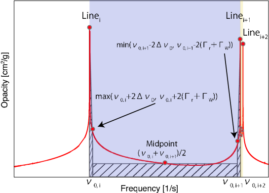
Figure 12.— Schematic line profile of SiO (red line) with illustration for selecting grids (red points) to calculate the SiO mean opacity. In the yellow-colored (blue-colored) region, the interval between two adjacent lines is smaller (larger) than $2\Delta\nu_{D}$ and (or) $2(\Gamma_{r}+\Gamma_{W})$. For example, the opacity integrated between $\nu_{0,i}$ and $\nu_{0,i+1}$ is approximated to be the sum of the areas of three shaded boxes.

References

- Allard et al. (2000) Allard, F., Hauschildt, P. H., & Schwenke, D. 2000, ApJ, 540, 1005
- Asimov & Ghiorso (1998) Asimov, P. D., & Ghiorso, M. S. 1998, American Mineralogist, 83, 1127
- Barnes et al. (2010) Barnes, R., Raymond, S. N., Greenberg, R., Jackson, B., & Kaib, N. A. 2010, ApJ, 709, L95
- Barton et al. (2013) Barton, E. J., Yurchenko, S. N., & Tennyson, J. 2013, MNRAS, 434, 1469
- Batalha et al. (2011) Batalha, N. M., et al. 2011, ApJ, 729, 27
- Bean et al. (2010) Bean, J. L., Miller-Ricci Kempton, E., & Homeier, D. 2010, Nature, 468, 669
- Birkby et al. (2013) Birkby, J. L., de Kok, R. J., Brogi, M., de Mooij, E. J. W., Schwarz, H., Albrecht, S., & Snellen, I. A. G. 2013, MNRAS, 436, L35
- Brogi et al. (2012) Brogi, M., Snellen, I. A. G., de Kok, R. J., Albrecht, S., Birkby, J., & de Mooij, E. J. W. 2012, Nature, 486, 502
- Bruntt et al. (2010) Bruntt, H., et al. 2010, A&A, 519, A51
- Clampin (2008) Clampin, M. 2008, in Society of Photo-Optical Instrumentation Engineers (SPIE) Conference Series, Vol. 7010, Society of Photo-Optical Instrumentation Engineers (SPIE) Conference Series
- Clanton et al. (2012) Clanton, C., Beichman, C., Vasisht, G., Smith, R., & Gaudi, B. S. 2012, PASP, 124, 700
- CRC Handbook (2011) CRC Handbook. 2011, CRC Handbook of Chemistry and Physics, 92nd Edition
- de Kok et al. (2013) de Kok, R. J., Brogi, M., Snellen, I. A. G., Birkby, J., Albrecht, S., & de Mooij, E. J. W. 2013, A&A, 554, A82
- Deming et al. (2007) Deming, D., Harrington, J., Laughlin, G., Seager, S., Navarro, S. B., Bowman, W. C., & Horning, K. 2007, ApJ, 667, L199
- Demory et al. (2012) Demory, B.-O., Gillon, M., Seager, S., Benneke, B., Deming, D., & Jackson, B. 2012, ApJ, 751, L28
- Deroo et al. (2012) Deroo, P., Swain, M. R., & Green, R. O. 2012, in Society of Photo-Optical Instrumentation Engineers (SPIE) Conference Series, Vol. 8442, Society of Photo-Optical Instrumentation Engineers (SPIE) Conference Series
- Dragomir et al. (2014) Dragomir, D., Matthews, J. M., Winn, J. N., & Rowe, J. F. 2014, in IAU Symposium, Vol. 293, IAU Symposium, ed. N. Haghighipour, 52
- Dumusque et al. (2014) Dumusque, X., et al. 2014, ApJ, 789, 154
- Ehrenreich et al. (2012) Ehrenreich, D., et al. 2012, A&A, 547, A18
- Fegley & Cameron (1987) Fegley, B., & Cameron, A. G. W. 1987, Earth and Planetary Science Letters, 82, 207
- Fortney et al. (2007) Fortney, J. J., Marley, M. S., & Barnes, J. W. 2007, ApJ, 659, 1661
- Fressin et al. (2013) Fressin, F., et al. 2013, ApJ, 766, 81
- Fressin et al. (2011) Fressin, F., et al. 2011, ApJS, 197, 5
- Ghiorso & Sack (1995) Ghiorso, M. S., & Sack, R. O. 1995, Contributions to Mineralogy and Petrology, 119, 197
- Gordon & McBride (1996) Gordon, S., & McBride, B. J. 1996, NASA Reference Publication 1311
- Grasset et al. (2009) Grasset, O., Schneider, J., & Sotin, C. 2009, ApJ, 693, 722
- Gray (1976) Gray, D. F. 1976, The observation and analysis of stellar photospheres
- Hatzes et al. (2011) Hatzes, A. P., et al. 2011, ApJ, 743, 75
- Henning et al. (2009) Henning, W. G., O’Connell, R. J., & Sasselov, D. D. 2009, ApJ, 707, 1000
- Howard et al. (2013) Howard, A. W., et al. 2013, Nature, 503, 381
- Irwin (1981) Irwin, A. W. 1981, ApJS, 45, 621
- Jolicard et al. (1997) Jolicard, G., Zucconi, J.-M., Drira, I., Spielfieldel, A., & Feautrier, N. 1997, J. Chem. Phys., 106, 10105
- Kawahara et al. (2014) Kawahara, H., Murakami, N., Matsuo, T., & Kotani, T. 2014, ApJS, 212, 27
- Kuntz (1997) Kuntz, M. 1997, J. Quant. Spec. Radiat. Transf., 57, 819
- Kurucz (1992) Kurucz, R. L. 1992, Rev. Mexicana Astron. Astrofis., 23, 45
- Kurucz & Avrett (1981) Kurucz, R. L., & Avrett, E. H. 1981, SAO Special Report, 391
- Léger et al. (2009) Léger, A., et al. 2009, A&A, 506, 287
- Lockwood et al. (2014) Lockwood, A. C., Johnson, J. A., Bender, C. F., Carr, J. S., Barman, T., Richert, A. J. W., & Blake, G. A. 2014, ApJ, 783, L29
- McDonough & Sun (1995) McDonough, & Sun. 1995, Chem. Geol., 120, 223
- Miguel et al. (2011) Miguel, Y., Kaltenegger, L., Fegley, B., & Schaefer, L. 2011, ApJ, 742, L19
- Nelson et al. (2014) Nelson, B. E., Ford, E. B., Wright, J. T., Fischer, D. A., von Braun, K., Howard, A. W., Payne, M. J., & Dindar, S. 2014, MNRAS, 441, 442
- Piskunov & Kupka (2001) Piskunov, N., & Kupka, F. 2001, ApJ, 547, 1040
- Plez (1998) Plez, B. 1998, A&A, 337, 495
- Ricker et al. (2010) Ricker, G. R., et al. 2010, in Bulletin of the American Astronomical Society, Vol. 42, American Astronomical Society Meeting Abstracts 215, 450.06
- Rodler et al. (2013) Rodler, F., Kürster, M., & Barnes, J. R. 2013, Monthly Notices of the Royal Astronomical Society, 432, 1980
- Rodler et al. (2012) Rodler, F., Lopez-Morales, M., & Ribas, I. 2012, ApJ, 753, L25
- Rossi et al. (1985) Rossi, S. C. F., Maciel, W. J., & Benevides-Soares, P. 1985, A&A, 148, 93
- Rothman et al. (2013) Rothman, L. S., et al. 2013, J. Quant. Spec. Radiat. Transf., 130, 4
- Rudnick & Gao (2003) Rudnick, R. L., & Gao, S. 2003, Treatise on Geochemistry, 3, 1
- Rybicki & Lightman (1986) Rybicki, G. B., & Lightman, A. P. 1986, Radiative Processes in Astrophysics
- Schaefer & Fegley (2004) Schaefer, L., & Fegley, B. 2004, Icarus, 169, 216
- Schaefer & Fegley (2009) Schaefer, L., & Fegley, B. 2009, ApJ, 703, L113
- Tinetti et al. (2012) Tinetti, G., et al. 2012, Experimental Astronomy, 34, 311
- Toon et al. (1989) Toon, O. B., McKay, C. P., Ackerman, T. P., & Santhanam, K. 1989, J. Geophys. Res., 94, 16287
- Traub & Oppenheimer (2011) Traub, W. A., & Oppenheimer, B. R. 2011, Direct Imaging of Exoplanets, ed. S. Seager 111
- Unsold (1955) Unsold, A. 1955, Physik der Sternatmospharen, MIT besonderer Berucksichtigung der Sonne.
- Valencia et al. (2007) Valencia, D., Sasselov, D. D., & O’Connell, R. J. 2007, ApJ, 665, 1413
- Vorypaev (1981) Vorypaev, G. G. 1981, Journal of Applied Spectroscopy, 35, 1297
- Waldmann & Pascale (2014) Waldmann, I. P., & Pascale, E. 2014, ArXiv e-prints
- William et al. (1996) William, H. P., Brian, P. F., Saul, A. T., & Vetterling, W. T. 1996, Numerical Recipes in Fortran 77: The Art of Scientific Computing
- Winn et al. (2011) Winn, J. N., et al. 2011, ApJ, 737, L18