Collective mode evidence of high-spin bosonization in a trapped one-dimensional atomic Fermi gas with tunable spin

Abstract

We calculate the frequency of collective modes of a one-dimensional repulsively interacting Fermi gas with high-spin symmetry confined in harmonic traps at zero temperature. This is a system realizable with fermionic alkaline-earth-metal atoms such as ¹⁷³Yb, which displays an exact SU($\kappa$) spin symmetry with $\kappa\geqslant 2$ and behaves like a spinless interacting Bose gas in the limit of infinite spin components $\kappa\rightarrow\infty$, namely high-spin bosonization. We solve the homogeneous equation of state of the high-spin Fermi system by using Bethe ansatz technique and obtain the density distribution in harmonic traps based on local density approximation. The frequency of collective modes is calculated by exactly solving the zero-temperature hydrodynamic equation. In the limit of large number of spin-components, we show that the mode frequency of the system approaches to that of a one-dimensional spinless interacting Bose gas, as a result of high-spin bosonization. Our prediction of collective modes is in excellent agreement with a very recent measurement for a Fermi gas of ¹⁷³Yb atoms with tunable spin confined in a two-dimensional tight optical lattice.

I Introduction

Ultracold atomic gases appear to be a versatile tool for discovering new phenomena and exploring new horizons in diverse branches of physics. To large extent, this is due to their unprecedented controllability and purity. A vast range of interactions, geometries and dimensions is possible: using the tool of Feshbach resonances FR and applying a magnetic field at the right strength, one can control very accurately the interactions between atoms, from arbitrarily weak to arbitrarily strong. By using the technique of optical lattices that trap atoms in crystal-like structures OpticalLattice , one can create artificial one- or two-dimensional environments to explore how physics changes with dimensionality. Most recently, it is also able to control the number of spin-components: degenerate Fermi gas with high-spin symmetry has been observed in alkaline-earth-metal atoms Yb Fukuhara2007 ; YbLENS .

The ytterbium (Yb) atom has a unique advantage in studying high-spin physics. It has a closed-shell electronic structure in the ground state, and hence its total spin is determined entirely by the nuclear spin, $I$. For the fermionic species ¹⁷³Yb, the nuclear spin is $I=5/2$ and the atom can be in six different internal states $\kappa=2I+1=6$. This gives rise to a unique feature of ¹⁷³Yb atom, that is, one simple internal-state-independent $s$-wave scattering length due to the absence of electronic spin in the atomic ground state Kitagawa2008 . Thus, the system exhibits SU(6) symmetry Hermele2009 ; Cazalilla2009 ; Gorshkov2010 . In such a high-spin system, possible novel ground states and topological excitations have been addressed theoretically Hermele2009 ; Cazalilla2009 ; Gorshkov2010 ; Wu2003 . One dimensional (1D) repulsively interacting fermions with sufficiently high spin also behave like spinless interacting Bose atoms Yang2011 , a phenomenon that we may refer to as high-spin bosonization. Physically, this phenomenon may also occur in two or three dimensions.

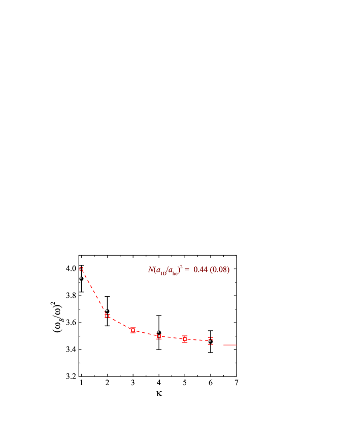
Figure 1: (Color online) Breathing mode frequency as a function of the number of components at the dimensionless interaction parameter $Na_{1D}^{2}/a_{ho}^{2}=0.44\pm 0.08$. The solid circles with error bars are the experimental data reported by the LENS team YbLENS . The empty squares are the theoretical results, with error bars counting for the experimental uncertainty for interaction parameter. The thin horizontal line at the right part of the figure shows the theoretical prediction at the infinitely large number of components. Source: Adapted from Ref. YbLENS . Copyright 2014, by Nature Publishing Group.

Experimentally, Fermi degeneracy of ¹⁷¹Yb and ¹⁷³Yb atoms has been demonstrated Fukuhara2007 ; Taie2010 ; YbLENS . In particular, in a very recent experiment performed at European Laboratory for Non-Linear Spectroscopy (LENS), a Fermi gas of ¹⁷³Yb atoms has been created in one-dimensional harmonic traps by using optical lattices and its momentum distribution and breathing mode oscillation have been measured YbLENS .

In this work, motivated by the recent measurement at LENS YbLENS , we investigate a 1D high-spin Fermi gas with strongly repulsive interactions satisfying SU($\kappa$) symmetry, by using exact Bethe ansatz technique beyond the mean-field framework Sutherland1968 . First, we solve the exact ground state of a homogeneous Fermi gas at zero temperature based on Bethe ansatz. To make contact with the experiment, we then consider an inhomogeneous Fermi cloud under harmonic confinement, within the framework of local density approximation (LDA). The equation of state of the system and the density distribution are calculated. By solving the zero-temperature hydrodynamic equation, we predict the frequency of low-lying collective modes. The main outcome of our research is summarized in Fig. 1, which shows the predicted breathing mode frequency in comparison with the recent data reported by LENS group, for a trapped ¹⁷³Yb gas at a dimensionless interaction parameter $Na_{1D}^{2}/a_{ho}^{2}=0.44\pm 0.08$ YbLENS . Here, $N$ is the total number of atoms in the Fermi cloud, $a_{1D}$ and $a_{ho}$ are the 1D s-wave scattering length and the length of harmonic oscillator, respectively. We find an excellent agreement between our theoretical prediction and the experimental data, with a relative discrepancy at a few percents. Fig. 1 has been published in Ref. YbLENS . The purpose of this paper is to present the details of our calculations, focusing particularly on the high-spin bosonization.

We note that in earlier works 1D multi-component Fermi gases with large-spin and attractive interactions have been discussed in detail amulti1 ; amulti2 . However, for repulsive interactions, only homogeneous Fermi gas in weak and strong coupling limits has been considered rmulti . Comparing with the case with attractive interactions there are no multi-component bound clusters in repulsively interacting Fermi gases.

The paper is organized as follows. In the following section, we describe briefly the model Hamiltonian. In Sec. III, we present the exact Bethe ansatz solution and discuss the equation of state and sound velocity of a uniform Fermi gas at zero temperature. Then, by using LDA in Sec. IV we determine the density distribution in the trapped environment. In Sec. V, we describe the dynamics of trapped Fermi gases in terms of 1D hydrodynamic equation. The behavior of low-lying collective modes is obtained and discussed. Finally, we conclude in Sec. VI.

II Model Hamiltonian

We consider a 1D multi-component Fermi gas with pseudo-spin $S=\left(\kappa-1\right)/2$, where $\kappa$ ($\geq 2$) is the number of components. The fermions in different spin states repulsively interact with each other via the same short-range potential $g_{1D}\delta(x)$. The first-quantized Hamiltonian with a total number of atoms $N=\sum_{l=1}^{\kappa}N_{l}$ (where $N_{l}$ is the number of fermions in the pseudo-spin state $l$) for the system is

$${\cal H}=\sum_{i=1}^{N}\left(-\frac{\hbar^{2}}{2m}\partial_{x_{i}}^{2}+V_{i}\right)+g_{1D}\sum_{i<j}\delta\left(x_{i}-x_{j}\right),$$ (1)

where $V_{i}=m\omega^{2}x_{i}^{2}/2$ is the harmonic trapping potential for the atom $i$ and $\omega$ is the trapping frequency. In general, such a 1D Fermi system is created by loading a 3D cloud into a tight 2D optical lattice and separating it into a number of highly elongated tubes. In each tube, it is convenient to express 1D coupling constant $g_{1D}$ in terms of an effective 1D scattering length,

$$g_{1D}=-\frac{2\hbar^{2}}{ma_{1D}},$$ (2)

where the effective 1D scattering length $a_{1D}$ is related to the 3D scattering length $a_{3D}$ by the relation Olshanni1998 ; Bergeman2003 ; Astrakharchik2004 ,

$$a_{1D}=-\frac{a_{\rho}^{2}}{a_{3D}}\left(1-\mathcal{A}\frac{a_{3D}}{a_{\rho}}\right)<0.$$ (3)

Here, $a_{\rho}=\sqrt{\hbar/(m\omega_{\rho})}$ is the characteristic oscillator length with transverse frequency $\omega_{\rho}$ determined by optical lattice depth and

$$\mathcal{A}\equiv-\frac{\zeta(1/2)}{\sqrt{2}}\simeq 1.0326$$ (4)

is a constant.

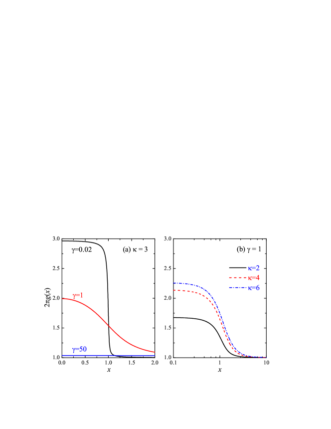
Figure 2: (Color online) Dependence of the quasi-momentum distribution $g\left(x\right)$ on the interaction strength (a) and on the number of components (b). At $x=0$, $g(x)$ increases with decreasing the interaction strength or increasing the number of spin-components. While at large $x$, $g(x)$ saturates to $1/2\pi$.

III Homogeneous equation of state

Let us first address a 1D uniform multi-component Fermi gas with symmetric inter-component interactions, i.e., there is no trapping potential term $V_{i}$ in the Hamiltonian (1). In this case, the model Hamiltonian is exactly soluble via the Bethe ansatz technique Sutherland1968 . Focusing on the experiment at LENS, we assume that each component has the same number of particles, i.e., $N_{l}=N/\kappa$ for $l=1,2,\cdots,\kappa=2S+1$. In free space, we measure the interactions by a dimensionless coupling constant

$$\gamma\equiv-\frac{mg_{1D}}{\hbar^{2}n}=\frac{2}{na_{1D}},$$ (5)

where $n$ is the linear total number density amulti2 . The ground state energy $E_{\hom}$ in the thermodynamic limit is given by Sutherland1968 ; rmulti ,

$$\frac{E_{\hom}}{L}=\frac{\hbar^{2}}{m}\left(\frac{n\gamma}{\lambda}\right)^{3}\int\limits_{0}^{1}x^{2}g\left(x\right)dx,$$ (6)

where

$$\lambda=2\gamma\int_{0}^{1}g\left(x\right)dx$$ (7)

and the quasi-momentum distribution $g\left(x\right)$ with $x\geq 0$ is determined by an integral equation

$$g\left(x\right) = \frac{\kappa}{2\pi}-\frac{1}{\pi}\sum\limits_{l=1}^{\kappa-1}\int\limits_{1}^{\infty}g\left(x^{\prime}\right)dx^{\prime}\left[\frac{l\lambda}{\left(l\lambda\right)^{2}+\left(x-x^{\prime}\right)^{2}}\right.$$ (8)

$$\left.+\frac{l\lambda}{\left(l\lambda\right)^{2}+\left(x+x^{\prime}\right)^{2}}\right].$$

The above Bethe ansatz equations are very similar to those for attractive interactions amulti1 ; amulti2 ; takahashi1 ; takahashi2 , but without the contribution from $\kappa$-body bound cluster states. In Fig. 3, we show the quasi-momentum distribution $g\left(x\right)$ for typical interaction parameters and the number of spin components, obtained by solving the integral equation Eq. (8), together with Eq. (7).

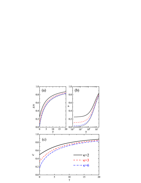
Figure 3: (Color online) Dependence of the uniform ground state energy per particle (a), the chemical potential (b), and the velocity of sound (c) on the dimensionless coupling constant $\gamma$, at several number of species as indicated. The energy per particle and sound velocity are in units of the energy $\pi^{2}[\hbar^{2}n^{2}/(2m)]$ and the velocity $\pi(\hbar n/m)$, respectively. Thin solid lines in (a) and (b) are the results of a 1D spinless interacting Bose gas with the same density $n$ and coupling constant $\gamma$. Note that in (b) for chemical potential, $\gamma$ is shown in the logarithmic scale. Thus, the saturation to the strongly interacting Tonk-Girardeau limit is not obvious.

Once we obtain the ground state energy by using the Bethe ansatz technique, we calculate the chemical potential by $\mu_{\hom}=\partial E_{\hom}/\partial N$ and the corresponding sound velocity by $c_{\hom}=\sqrt{n(\partial\mu_{\hom}/\partial n)/m}$. For numerical purposes, it is convenient to rewrite these thermodynamic quantities in a dimensionless form that depends on the coupling constant $\gamma$ only,

$$\frac{E_{\hom}}{L} \equiv \frac{\hbar^{2}n^{3}}{2m}e\left(\gamma\right),$$ (9)

$$\mu_{\hom} \equiv \frac{\hbar^{2}n^{2}}{2m}\mu\left(\gamma\right),$$ (10)

$$c_{\hom} \equiv \frac{\hbar n}{m}c\left(\gamma\right).$$ (11)

These dimensionless functions are related by,

$$\mu\left(\gamma\right) = 3e\left(\gamma\right)-\gamma\frac{\partial e\left(\gamma\right)}{\partial\gamma},$$ (12)

$$c\left(\gamma\right) = \sqrt{\mu\left(\gamma\right)-\frac{\gamma}{2}\frac{\partial\mu\left(\gamma\right)}{\partial\gamma}}.$$ (13)

It is easy to see that for an ideal, non-interacting multi-component Fermi gas,

$$\frac{E_{\hom}^{ideal}}{L} =\frac{\hbar^{2}n^{3}}{2m}\left(\pi^{2}/3\kappa^{2}\right),$$ (14)

$$\mu_{\hom}^{ideal} =\frac{\hbar^{2}n^{2}}{2m}\left(\pi^{2}/\kappa^{2}\right),$$ (15)

and

$$c_{\hom}^{ideal}=\frac{\hbar n}{m}\left(\pi/\kappa\right).$$ (16)

By numerically solving the integral Eqs. (6)-(8), we obtain the ground state energy per particle, chemical potential, and sound velocity as a function of the dimensionless coupling constant $\gamma$, as shown in Fig. 3. With increasing the coupling constant, the energy, chemical potential and sound velocity increase rapidly from the ideal gas results and finally saturate to the strongly interacting Tonk-Girardeau gas limit, as one may anticipate. With increasing the number of components $\kappa$, these thermodynamic quantities decrease instead. It is interesting that for a sufficiently large number of components, they approach to the results of a 1D repulsively interacting spinless Bose gas with the same total density $n$ and the coupling constant $\gamma=-mg_{1D}/(\hbar^{2}n)$, which are obtained by solving the following integral equation takahashi1 ,

$$f\left(k\right)=\frac{1}{2\pi}+\frac{1}{\pi}\intop_{-1}^{+1}\frac{\lambda_{B}^{2}}{\lambda_{B}^{2}+\left(k-k^{\prime}\right)}f\left(k^{\prime}\right)dk^{\prime},$$ (17)

together with the normalization condition

$$\lambda_{B}=2\gamma\intop_{0}^{1}f\left(k\right)dk$$ (18)

and the expression for the energy

$$\frac{E_{\hom}^{B}}{L}=\frac{\hbar^{2}}{m}\left(\frac{n\gamma}{\lambda_{B}}\right)^{3}\int\limits_{0}^{1}k^{2}f\left(k\right)dk.$$ (19)

The equivalence between high-spin Fermi gas and spinless Bose gas, namely high-spin bosonization, has been analytically shown by Yang and You Yang2011 . This is an interesting counterpart of the 1D effective fermionization for strongly interacting particles in one dimension Cazalilla2011 .

IV Density distribution in harmonic traps

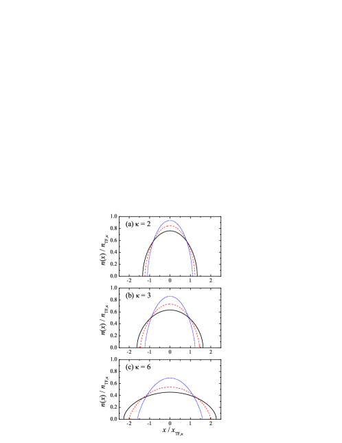
Figure 4: (Color online) Density distributions of a 1D trapped multi-component Fermi cloud at three interaction parameters $Na_{1D}^{2}/a_{ho}^{2}=0.1$ (black solid line), $1$ (red dashed line), and $10$ (blue dotted line). The linear density and the coordinate are in units of the peak density $n_{TF,\kappa}$ and Thomas-Fermi radius $x_{TF,\kappa}$ of an ideal Fermi gas, respectively.

To make quantitative contact with the experiment at LENS YbLENS , it is crucial to take into account the external harmonic trapping potential $V(x)=m\omega^{2}x^{2}/2$, which is necessary to prevent the fermions from escaping. We define a dimensionless parameter $\delta=Na_{1D}^{2}/a_{ho}^{2}$ to describe the interactions Astrakharchik2004 ; amulti2 . Here $a_{ho}=\sqrt{\hbar/(m\omega)}$ is the characteristic oscillator length in the axial direction. It is somehow counterintuitive that $\delta\gg 1$ corresponds to the weakly coupling limit, while $\delta\ll 1$ corresponds to the strongly interacting regime. For a large number of fermions, which is about $N\sim 50$ experimentally YbLENS , an efficient way to take the trap into account is by using the local density approximation (LDA). Together with the exact homogeneous equation of state of a 1D multi-component Fermi gas, this gives an asymptotically exact results as long as $N\gg 1$. The LDA amounts to determining the chemical potential $\mu$ from the local equilibrium condition Astrakharchik2004 ; ldh1d ; hld1d ,

$$\mu_{\hom}\left[n(x)\right]+\frac{1}{2}m\omega^{2}x^{2}=\mu_{g},$$ (20)

under the normalization restriction $N=\int_{-x_{F}}^{+x_{F}}n\left(x\right)dx$, where $n\left(x\right)$ is the total linear number density and is nonzero inside a radius $x_{F}$. We have used the subscript “$g$” to distinguish the global chemical potential $\mu_{g}$ from the local chemical potential $\mu_{\hom}$. Rewriting $\mu_{\hom}$ into the dimensionless form $\mu[\gamma\left(x\right)]$ and $\gamma\left(x\right)=2/[n\left(x\right)a_{1D}]$, we find that

$$\frac{\hbar^{2}n^{2}\left(x\right)}{2m}\mu\left[\gamma\left(x\right)\right]+\frac{1}{2}m\omega^{2}x^{2}=\mu_{g}.$$ (21)

We solve the above LDA equations numerically amulti2 .

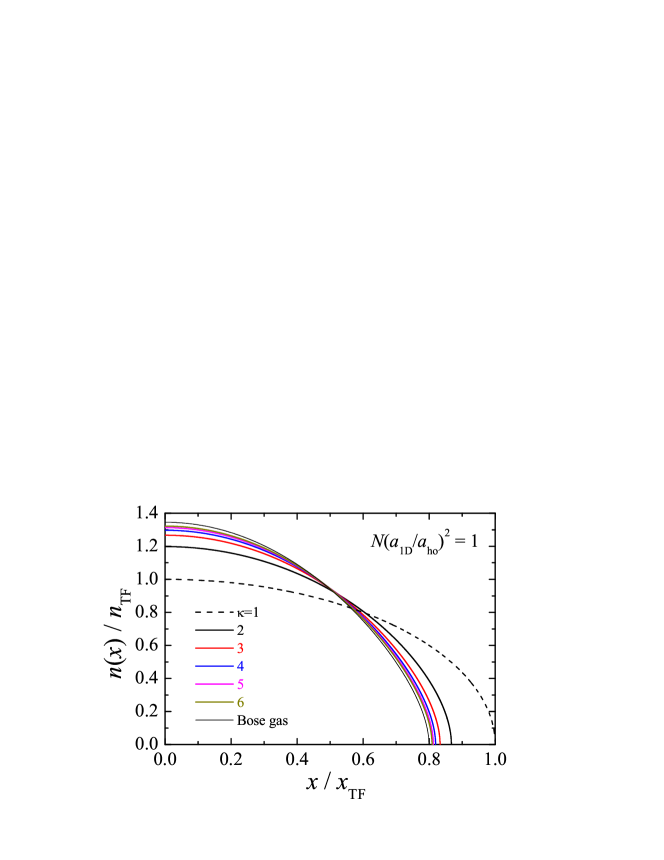
Figure 5: (Color online) Evolution of density distributions with increasing the number of components at the interaction parameter $Na_{1D}^{2}/a_{ho}^{2}=1$.

Fig. 4 reports the numerical results of the density distributions at different number of component $\kappa$ and at three typical interaction parameters $Na_{1D}^{2}/a_{ho}^{2}$. The linear density and the coordinate are in units of the peak density $n_{TF,\kappa}=\sqrt{2N\kappa}/\left(\pi a_{ho}\right)$ and the Thomas-Fermi radius $x_{TF,\kappa}=\sqrt{2N/\kappa}a_{ho}$ of an ideal gas, respectively. With increasing interaction parameter as shown in each panel, the density distribution changes from an ideal gas distribution to a strongly interacting Tonks-Girardeau profile. At the same interaction parameter, the density distribution become flatter and broader as the number of components $\kappa$ increases.

To show explicitly the effect of high-spin bosonization, in Fig. 5 we plot again the density distributions of $\kappa$-component Fermi gas with varying $\kappa$ at a given dimensionless interaction parameter $Na_{1D}^{2}/a_{ho}^{2}=1$, and compare them with the result of an interacting spinless Bose gas, which is obtained by replacing $\mu_{\textrm{hom}}$ with $\mu_{\textrm{hom}}^{B}=\partial E_{\textrm{hom}}^{B}/\partial N$ (see Eq. (19) for $E_{\textrm{hom}}^{B}$) note . The profiles are shown in units of the peak density $n_{TF}=\sqrt{2N}/\left(\pi a_{ho}\right)$ and the Thomas-Fermi radius $x_{TF}=\sqrt{2N}a_{ho}$, for the purpose of comparison. With increasing $\kappa$, the profiles converge quickly to the density distribution of an interacting spinless Bose gas (thin line), as a result of high-spin bosonization.

V Low-lying collective modes

Experimentally, a useful way to characterize an interacting system is to measure its low-lying collective excitations of density oscillations Hu2004 . Quantitative calculations of the low-lying collective excitations in traps can be based on the superfluid hydrodynamic description of the dynamics of the 1D Fermi gas stringari . In such a description, the density $n\left(x,t\right)$ and the velocity field $v\left(x,t\right)$ satisfy the equation of continuity

$$\frac{\partial n\left(x,t\right)}{\partial t}+\frac{\partial}{\partial x}\left[n\left(x,t\right)v\left(x,t\right)\right]=0,$$ (22)

and the Euler equation

$$m\frac{\partial v}{\partial t}{\bf+}\frac{\partial}{\partial x}\left[\mu_{\hom}\left(n\right)+V_{trap}\left(x\right)+\frac{1}{2}mv^{2}\right]=0.$$ (23)

We consider the fluctuations of the density and the velocity field about the equilibrium ground state , $\delta n\left(x,t\right)=$ $n\left(x,t\right)-n(x)$ and $\delta v\left(x,t\right)=v\left(x,t\right)-v(x)=v\left(x,t\right)$, where $n(x)$ and $v(x)\equiv 0$ are the equilibrium density profile and velocity field. Linearizing the hydrodynamic equations, one finds that stringari ,

$$\frac{\partial^{2}}{\partial t^{2}}\delta n\left(x,t\right)=\frac{1}{m}\frac{\partial}{\partial x}\left\{n\frac{\partial}{\partial x}\left[\frac{\partial\mu_{\hom}(n)}{\partial n}\delta n\left(x,t\right)\right]\right\}.$$ (24)

The boundary condition requires that the current $J(x,t)=n(x)\delta v\left(x,t\right)$ should vanish identically at the Thomas-Fermi radius $x=\pm x_{TF}$. Considering the $j$-th eigenmode with $\delta n\left(x,t\right)=\delta n\left(x\right)\exp\left[i\omega_{j}t\right]$ and removing the time-dependence, we end up with an eigenvalue problem, i.e.,

$$\frac{1}{m}\frac{d}{dx}\left\{n\frac{d}{dx}\left[\frac{\partial\mu_{\hom}(n)}{\partial n}\delta n\left(x\right)\right]\right\}+\omega_{j}^{2}\delta n\left(x\right)=0.$$ (25)

We note that the above hydrodynamic description is applicable in a collisional regime characterized by the condition $N(1-\mathcal{T})\gg 1$, where $\mathcal{T}$ is the transmission coefficient for a 1D collision of two fermionic atoms along the $x$-direction Olshanni1998 . The calculation of the transmission coefficient $\mathcal{T}$ has been given by Olshanni in his seminal work Olshanni1998 . By estimating a collision wavevector $k_{z}\sim k_{F}$ and by using the experimental parameters $N\sim 100$ and $a_{\rho}/a_{3D}\simeq 4.5$ at LENS YbLENS , we find that $\mathcal{T}\sim 0.3$ and $N(1-\mathcal{T})\sim 70\gg 1$. Hence, the collisional regime is well reached in the recent LENS experiment YbLENS .

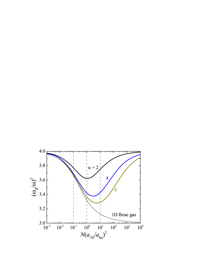
Figure 6: (Color online) Breathing mode frequency as a function of the dimensionless interaction parameter at different number of components. In the infinitely large number of components, the mode frequency will approach to that of a 1D interacting spinless Bose gas (thin line).

To solve the hydrodynamic equation (25), we use the powerful multi-series-expansion method developed in Ref. amulti2 . The resulting low-lying collective mode can be classified by the number of nodes in its eigenfunction, i.e., the number index “$j$”. The lowest two modes with $j=1,2$ are the dipole and breathing (compressional) modes, respectively, which can be excited separately by shifting the trap center or modulating the harmonic trapping frequency. The dipole mode is not affected by interactions according to Kohn’s theorem, and has an invariant frequency precisely at $\omega_{1}=\omega$. Therefore, the mode frequency of the breathing mode provides the first means to probe the non-trivial thermodynamics of our interacting system.

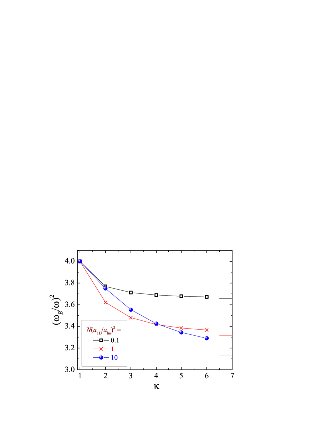
Figure 7: (Color online) Illustration of high-spin bosonization in breathing mode frequency. Here we show the evolution of breathing mode frequency as a function of the number of components at the interaction strength $Na_{1D}^{2}/a_{ho}^{2}=0.1$ (black empty squares), $1$ (red crosses), and $10$ (blue solid circles). With increasing the number of components, the breathing mode frequency approaches to the frequency of a 1D interacting spinless Bose gas (thin lines).

In Fig. 6, we show the breathing mode frequency as a function of the dimensionless interaction parameter $\delta=Na_{1D}^{2}/a_{ho}^{2}$ at different number of components $\kappa$. In the weak coupling limit ($\delta\gg 1$) the cloud behaves likes an ideal Fermi gas, whose breathing mode frequency is $2\omega$. In the strongly interacting Tonks-Girardeau limit ($\delta\ll 1$), the cloud is fermionized and the mode frequency is again given by $2\omega$. Therefore, for a given number of components, the breathing mode frequency exhibits an interesting dip when the system crosses from the weak over to the strong coupling regime. We note that for $\kappa=2$, such a dip structure was predicted earlier by using a sum-rule approach Astrakharchik2004 . With increasing the number of components $\kappa$, the mode frequency decreases and finally approaches to that of a 1D interacting spinless Bose gas. This high-spin bosonization behavior is highlighted in Fig. 7. It should be noted that the Bose gas limit is very difficult to reach in the weakly interacting regime when $\delta\gg 1$.

In Fig. 1, we compare our predictions for breathing mode frequency with the experimental data reported by the LENS team YbLENS . The experiment was performed at an average interaction parameter $Na_{1D}^{2}/a_{ho}^{2}=0.44\pm 0.08$. The solid circles with error bars are the experimental results. The empty squares with error bars are the theoretical results. The error bar in the theoretical result is due to the uncertainty in the interaction parameter $\Delta(Na_{1D}^{2}/a_{ho}^{2})=0.08$. The agreement between theory and experiment, within a relative discrepancy of a few percents, is impressive, as there is no any adjustable parameter. When the number of component increases, both theoretical and experimental data approach to the result of a 1D interacting spinless Bose gas, as indicated by a thin horizontal line at the right part of the figure. This could be viewed as an experimental proof of the high-spin bosonization phenomenon.

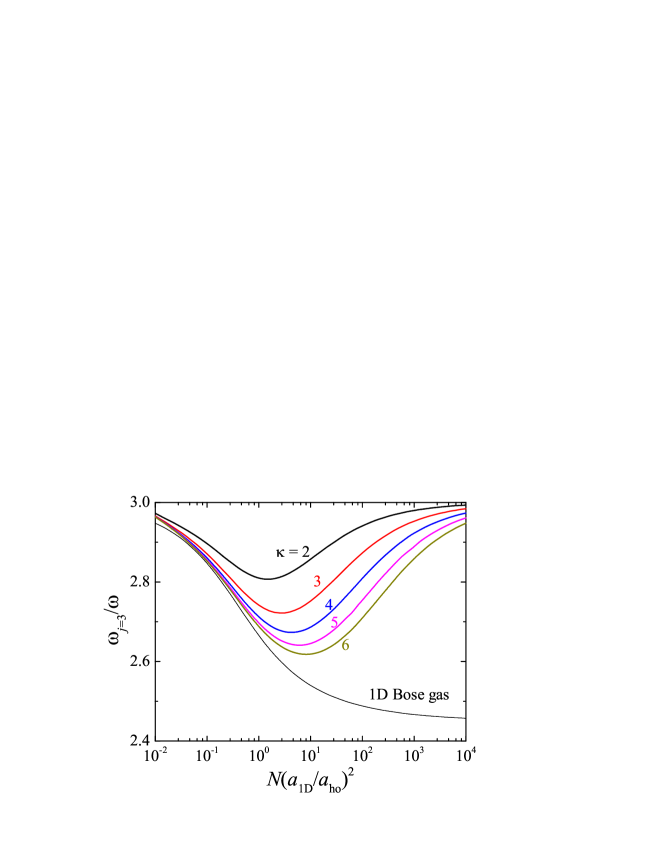
Figure 8: (Color online) The 3rd mode frequency as a function of the dimensionless interaction parameter at different number of components. In the infinitely large number of components, the mode frequency will approach to that of a 1D interacting spinless Bose gas (thin line).

Qualitatively, collective modes with larger number of nodes ($j>2$) exhibit the same feature as the breathing mode. An example is shown in Fig. 8, for the frequency of the third collective mode. Experimentally, however, these modes are more difficult to excite and measure.

VI Conclusion

In summary, we have investigated the thermodynamics and collective modes of 1D repulsively interacting Fermi gases with high-spin symmetry, based on the exact Bethe ansatz technique beyond the mean-field method, in a homogeneous environment. This has been extended to include a harmonic trap, by using the local density approximation. The equation of state of the system has been discussed in detail, as well as some dynamical quantities, including the sound velocity and low-lying collective modes.

We have compared our collective mode prediction with a recent measurement performed at LENS in a Fermi gas of ¹⁷³Yb atoms, confined in one dimension by using two-dimensional optical lattice. We have found excellent quantitative agreement. In addition, we have predicted that as the number of spin components $\kappa$ increases, the mode frequency of the 1D repulsively interacting Femi gas approaches to that of a 1D interacting spinless Bose gas. This intriguing high-spin bosonization phenomenon is qualitatively verified in the experiment in the regime with an intermediate interaction strength.

References

(1) S. Inouye, M. R. Andrews, J. Stenger, H. -J. Miesner,
D. M. Stamper-Kurn, and W. Ketterle, Nature (London) 392,
151 (1998).
(2)M. Greiner, O. Mandel, T. Esslinger, T. W.
Hänsch, and I. Bloch, Nature (London) 415, 39 (2002).
(3)T. Fukuhara, Y. Takasu, M. Kumakura, and Y.
Takahashi, Phys. Rev. Lett. 98, 030401 (2007).
(4)S. Taie, Y. Takasu, S. Sugawa, R. Yamazaki, T.
Tsujimoto, R. Murakami, and Y. Takahashi, Phys. Rev. Lett. 105,
190401 (2010).
(5)G. Pagano, M. Mancini, G. Cappellini, P. Lombardi,
F. Schäfer, H. Hu, X.-J. Liu, J. Catani, C. Sias, M. Inguscio, and
L. Fallani, Nature Phys. 10, 198 (2014).
(6)M. Kitagawa, K. Enomoto, K. Kasa, Y. Takahashi,
R. Ciuryło, P. Naidon, and P. S. Julienne, Phys. Rev. A 77,
012719 (2008).
(7)M. Hermele, V. Gurarie, and A. M. Rey, Phys.
Rev. Lett. 103, 135301 (2009).
(8)M. A. Cazalilla, A. F. Ho, and M. Ueda, New
J. Phys. 11, 103033 (2009).
(9)A. V. Gorshkov, M. Hermele, V. Gurarie, C.
Xu, P. S. Julienne, J. Ye, P. Zoller, E. Demler, M. D. Lukin, and
A. M. Rey, Nature Phys. 6, 289 (2010).
(10)C. Wu, J.-P. Hu, and S.-C, Zhang, Phys. Rev. Lett.
91, 186402 (2003);
(11)C. N. Yang and Y. Z. You, Chin. Phys. Lett. 28,
020503 (2011).
(12)B. Sutherland, Phys. Rev. Lett. 20,
98 (1968).
(13)X.-W. Guan, M. T. Batchelor, C. Lee, and H. -Q.
Zhou, Phys. Rev. Lett. 100, 200401(2008).
(14)X.-J. Liu, H. Hu, and P. D. Drummond, Phys. Rev.
A, 77, 013622 (2008).
(15) X.-W. Guan, Z.-Q. Ma, and B. Wilson, Phys. Rev.
A, 85, 033633 (2012).
(16) M. Olshanni, Phys. Rev. Lett. 81, 938 (1998).
(17)T. Bergeman, M. G. Moore, and M. Olshanii,
Phys. Rev. Lett. 91, 163201 (2003).
(18) G. E. Astrakharchik, D. Blume, S. Giorgini,
and L. P. Pitaevskii, Phys. Rev. Lett. 93, 050402 (2004).
(19) M. Takahashi, Thermodynamics of One-Dimensional
Solvable Models (Cambridge University Press, Cambridge, 1999).
(20) M. Takahashi, Prog. Theor. Phys. 44,
899 (1970).
(21)M. A. Cazalilla, R. Citro, T. Giamarchi, E.
Orignac, and M. Rigol, Rev. Mod. Phys. 83, 1405 (2011).
(22) X.-J. Liu, P. D. Drummond, and H. Hu, Phys. Rev.
Lett. 94, 136406 (2005).
(23) H. Hu, X.-J. Liu, and P. D. Drummond, Phys. Rev.
Lett. 98, 070403 (2007).
(24)Similarly, all the results of a 1D interacting spinless
Bose gas, including the mode frequency that we will discuss later,
are obtained by replacing with ,
at the same total number of atoms and the coupling constant .
(25)H. Hu, A. Minguzzi, X.-J. Liu, and M. P. Tosi, Phys.
Rev. Lett. 93, 190403 (2004).
(26) C. Menotti and S. Stringari, Phys. Rev. A 66,
043610 (2002).